Kinetic energy of solid neon by Monte Carlo
with improved Trotter- and finite-size extrapolation

Abstract

The kinetic energy of solid neon is calculated by a path-integral Monte Carlo approach with a refined Trotter- and finite-size extrapolation. These accurate data present significant quantum effects up to temperature $T=20$ K. They confirm previous simulations and are consistent with recent experiments.

In a previous work [2] we reported theoretical results about the average kinetic energy of rare gas solids (krypton, argon and neon), modeled by a Lennard-Jones (LJ) interaction. For heavier crystals the thermodynamics was approached by means of the effective-potential method [3, 4]. This approach allows us the use of all classical methods through the construction of an approximate effective classical phase-space distribution (see for details [5]). Monte Carlo simulations [6, 7, 8, 9, 2] with the effective potential were favourably compared with path-integral Monte Carlo (PIMC) simulations, and also applied to argon [7], reproducing very well the experimental density and specific heat [10].

In spite of their large mass, krypton and argon show relevant quantum effects at easily accessible temperatures; for instance, the average kinetic energy is much larger than its corresponding classical value. Our calculations of the average kinetic energy of argon suggested the realization of neutron Compton scattering (NCS) experiments, whose outcomes have been later found in perfect agreement with our predictions [11]. For increasing value of the quantum coupling, anharmonic second order corrections arising from the odd part of the potential were found relevant [8] and have been recently inserted in the effective potential formalism [12].

For neon, where the strong anharmonicity shows up even in the ground state [13], we preferred to resort to path-integral Monte Carlo (PIMC) simulations, with a refined Trotter extrapolation [2]; the procedure consists in adding to the PIMC data the contribution of the harmonic approximation after the subtraction of the corresponding finite Trotter data.

The available experimental data for the kinetic energy of solid neon obtained by NCS experiments [14], were in evident disagreement with our PIMC results; all theoretical data were lower than the experimental ones. The reason was not clear at all. Since the experiments with argon [11] were not yet performed, we supposed that the LJ potential were an over-simplification of the true potential and that many-body interactions could play an important role.

In a recent work Timms et al. [15] report new NCS measurements of the kinetic energy of solid neon, which differ from the previous ones [14]. Both experiments were carried out and analyzed in the regime of the so-called impulse approximation, which becomes exact when the energy and the momentum transferred to the sample are infinite. Timms et al. reached higher momentum and energy transfers, and they claim that this improvement has made the final-state-effect corrections to the observed longitudinal Compton profile irrelevant: hence, the data analysis had less sources of uncertainty and was thus more reliable. They also did new PIMC simulations, using different potentials (Aziz and LJ) in order to definitively establish whether the original disagreement between theory and experiment was due to a too rough model potential: it turned out that the computed kinetic energy depends very weakly on the model potential. Their experimental and PIMC data are consistent between themselves, and also confirm the validity of our previous simulations.

In a recent paper [16] we have developed a systematic method for improving the Trotter number extrapolation of PIMC data; in addition, we have recently extended this procedure in order to take into account also the effect of the finite size of the simulation box [17], so that we are now able to obtain much more accurate results.

The PIMC method is based upon the semi-group property of the density matrix

$$\rho({\mbox{\boldmath$q$}}^{\prime},{\mbox{\boldmath$q$}};\beta)=\int d{\mbox{\boldmath$q$}}_{P-1}...d{\mbox{\boldmath$q$}}_{1}\rho({\mbox{\boldmath$q$}}^{\prime},{\mbox{\boldmath$q$}}_{P-1};\tau)...\rho({\mbox{\boldmath$q$}}_{1},{\mbox{\boldmath$q$}};\tau),$$ (1)

where $\beta=1/T$ and $\tau=\beta/P$, P being the Trotter number. In order to make the above formula of practical use, the density matrix element $\rho({\mbox{\boldmath$q$}}_{\ell},{\mbox{\boldmath$q$}}_{\ell-1};\tau)$ is usually taken in the lowest high-temperature approximation, giving rise to the so-called primitive action. The latter tends to the exact density matrix as $P\to\infty$. This is the formalism we are dealing with here. In order to get values of the averages of physical observables, many simulations at different values of $P$ must be performed, and then the data must be extrapolated as $P\to\infty$. The more “quantum” is the system, the larger must be the maximum value of $P$. The finite $P$ estimates $G(P)$ of the averages can be expanded as $G(P)=G(\infty)+g_{2}/P^{2}+g_{4}/P^{4}+\cdots$ [18], and frequently the term in $1/P^{2}$ is not sufficient for a satisfactory fit.

The method we suggested [16] overcomes this problem. The idea is to take advantage of the fact that the thermodynamics of a harmonic system can be obtained analytically, even at finite $P$ (see Ref. [19]); nevertheless, such a system shows a very strong dependence on $P$, and the results obtained at finite $P$ will not be close to those at $P=\infty$ unless the condition $P\gg{f}=\beta\hbar\omega/2$ is fulfilled for any system’s frequency $\omega$. However, at low temperatures, when quantum effects are most important (in the temperature region where one should use the highest values of $P$), the harmonic approximation (HA) of a solid system is surely meaningful, though rough. Indeed, as $T\to{0}$, harmonic excitations play a very important role in the thermodynamics. As long as the “quantum character” of the system increases, this becomes less and less true, but the self-consistent HA (SCHA) [20, 21] eventually allows to recover a simple harmonic-like system whose behaviour is very similar to that of the real system.

Our idea is to improve the extrapolation as $P\to\infty$ in PIMC simulations accounting for the $P$ dependence of the harmonic contributions to the PIMC estimates of physical observables. The procedure consists in adding to the rough PIMC data $G(P)$ the deviation from the $P=\infty$ estimates calculated for the SCHA of the system:

$$G_{SC}(P)=G(P)+\left[G_{SC}^{(h)}(\infty)-G_{SC}^{(h)}(P)\right]~{}.$$ (2)

In such a way, the improved estimates $G_{SC}(P)$ will show a much weaker dependence on the Trotter number $P$, the scaling behaviour in $1/P^{2}$ is reached earlier and the maximum Trotter number necessary to get the correct asymptotic result is lower. We remember that as $P$ increases the computer time grows both because of the larger simulation box and of the worse statistics.

Another important point which has not yet been deeply investigated in relation to quantum simulations is the dependence of the data on the simulation box size. It is well known that for systems undergoing a phase transition the finite size of the simulated sample has dramatic effects, because in the critical region the correlation length diverges, and in order to simulate such a system particular procedures known as “finite-size scaling” must be used. In the classical case, if the system is far from a phase transition, the problem of how to reach the thermodynamic limit regime is in general easily overcome, without using enormous samples (size effects, with modern computer capability, are in general not a problem). However, dealing with quantum systems, subtle phenomena can occur: for instance, in $d$-dimensional lattices the discreteness of the Brillouin zone due to the finite particle number introduces a nonphysical gap into the dispersion curve which gives rise, at low temperature, to an exponential behaviour of the specific heat, instead of the correct $T^{d}$ scaling Bloch law, obtained for a linear dispersion of the soft modes. This effect can be observed in simulations [13].

Following the idea of Eq. (2) we suggest [17] to correct the raw PIMC data, at the SCHA level, also with respect to their dependence on $N$, the number of particles composing the actually simulated sample,

$$G_{SC}(P,N)=G(P,N)+\left[G_{SC}^{(h)}(\infty,\infty)-G_{SC}^{(h)}(P,N)\right]~{}.$$ (3)

Preliminary tests [17] made on 1-d nonlinear systems confirm that even with a chain composed by very few particles it is possible to get the thermodynamic limit of the averages of observables only adding to the raw simulation data this harmonic-like correction, practically making the extrapolation as $N\to\infty$ unnecessary.

To model solid neon, we considered a fcc lattice composed by $N$ particles (labeled with 3-d indices i, j) interacting through a pairwise potential,

$$V({\mbox{\boldmath$q$}})=\frac{1}{2}\sum_{\bf ij}v\big{(}|{\mbox{\boldmath$q$}}_{{\bf i}}-{\mbox{\boldmath$q$}}_{\bf j}|\big{)}~{}.$$ (4)

Several choices, as we know, are possible for the model potential. Since Timms et al. [15] showed that the dependence of the kinetic energy on the potential is not critical, we chose to model our system by the LJ 12-6 potential $v(r)=4\varepsilon\big{[}(\sigma/r)^{12}-(\sigma/r)^{6}\big{]}$ with the potential parameters $\varepsilon$ and $\sigma$ taken from the literature [22] ($\varepsilon=36.68$ K and $\sigma=2.787$ Å). We neglect the dynamic effect of the interactions beyond nearest-neighbours, whose contribution to the potential energy is taken into account by a static-lattice approximation. We performed constant-density simulations evaluating the pressure within each run. The density was adjusted in such a way to get a practically vanishing pressure, (the pressure is always less than $0.07\,p^{*}\approx{15}$ atm, being $p^{*}=\varepsilon/\sigma^{3}$ the characteristic pressure) in order to best reproduce the experimental settings; the zero-pressure densities turned out to be very close to the experimental ones. The sample was an fcc lattice of $108$ atoms with periodic boundary conditions; in order to test the above described finite-size correction scheme we made test runs changing the box size up to $864$ particles. We used the Metropolis algorithm, with both single- and many-particle moves. The maximum Trotter number $P$ was $48$. Each run consisted of $200,000$ steps per particle for equilibration followed by $1,200,000$ further steps, during which the averages were accumulated every $5$ steps. For each run we estimated the statistical uncertainty, taking into account the MC correlation times; these vary with $P$ and $N$ and never exceed 400 steps.

In order to make finite-Trotter and finite-size harmonic corrections in the spirit described above, we need the SCHA potential,

$$V_{0}({\mbox{\boldmath$q$}})=\frac{1}{2}Nzw+\frac{1}{2}m\sum_{{\bf i}\alpha}\sum_{{\bf j}\beta}{\Omega^{2}}_{\bf ij}^{\alpha\beta}\xi_{\bf i}^{\alpha}\xi_{\bf j}^{\beta}~{},$$ (5)

where $\xi_{\bf i}^{\alpha}=q_{\bf{i}}^{\alpha}-q_{0,{\bf i}}^{\alpha}$ and ${\bf{q}}_{0,{\bf{i}}}$ is the equilibrium position of the $i-th$ particle, which is fixed, being determined by the particle density. $z=12$ is the coordination number and $w$ and ${\Omega^{2}}_{\bf{ij}}^{\alpha\beta}$ are adjustable parameters determined imposing that the average of the actual potential $V({\mbox{\boldmath$q$}})$, and of its first and second derivatives are equal to the corresponding averages obtained for $V_{0}({\mbox{\boldmath$q$}})$: all averages are performed using the finite-$P$ density distribution corresponding to $V_{0}({\mbox{\boldmath$q$}})$, which is a gaussian. A shorthand way of expressing these gaussian averages as a formal power series turns out to be very useful in this case, namely $\big{\langle}{f}(\mbox{\boldmath$\xi$}_{\bf{id}})\big{\rangle}_{0}\equiv\exp({\cal{D}}^{\alpha\beta}\partial_{\alpha}\partial_{\beta}/2)\,f({\bf{0}})$ (summation over repeated indices) where $\mbox{\boldmath$\xi$}_{\bf{id}}\equiv\mbox{\boldmath$\xi$}_{{\bf{i}}+{\bf{d}}}{-}\mbox{\boldmath$\xi$}_{\bf{i}}$ (d labels the nearest-neighbour displacements) and ${\cal D}^{\alpha\beta}=\big{\langle}\xi_{\bf{id}}^{\alpha}\xi_{\bf{id}}^{\beta}\big{\rangle}_{0}$ is the variance matrix of the gaussian distribution.

Since $v(r)\to\infty$ as $r$ approaches $0$, averages like $\big{\langle}{v}\big{(}|{\bf{d}}{+}\mbox{\boldmath$\xi$}_{\bf{id}}|\big{)}\big{\rangle}_{0}$ would diverge. This is an artifact of the harmonic approximation: the gaussian is small but nonzero at $r=0$, where the true distribution would vanish; the formal power series $\exp({\cal D}^{\alpha\beta}\partial_{\alpha}\partial_{\beta}/2)V({\mbox{\boldmath$q$}})$ is then only asymptotic. However, the nonphysical contributions from the potential core can be simply eliminated by truncating the series. Hence we can expand the averaged potential and its derivatives up to second order in the ${\cal D}^{\prime}s$, finally obtaining the following SCHA equations

$${m\,{\Omega^{2}}_{\bf k}^{\nu}\over 2} = \tilde{v}^{\prime\prime}\big{(}\nu_{\bf{k}}^{2}+A_{\bf{k}}^{\nu}\big{)}+{\tilde{v}^{\prime}\over d}\big{(}\nu_{\bf{k}}^{2}-A_{\bf{k}}^{\nu}\big{)}$$ (8)

$$w=v+{1\over 4}\bigg{[}\big{(}v^{\prime\prime}+\tilde{v}^{\prime\prime}\big{)}{\cal{D}}_{\|}+\Big{(}{v^{\prime}\over d}+{\tilde{v}^{\prime}\over d}\Big{)}{\cal{D}}_{\perp}\bigg{]}$$

$$\hskip 85.35826pt-\frac{1}{Nz}\sum_{{\bf k}\nu}m{\Omega^{2}}_{\bf k}^{\nu}\alpha_{\bf k}^{\nu}~{},$$

where $v\equiv{v}(d)$, $v^{\prime}\equiv{v^{\prime}}(d)$ and so on; $d\equiv|{\bf d}|$ is the nearest-neighbour distance. The indices ${\bf{k}}$ (wavevector) and $\nu$ (polarization) label the normal modes, obtained by diagonalizing ${\Omega^{2}}_{\bf ij}^{\alpha\beta}$ to the eigenfrequencies ${\Omega^{2}}_{\bf{k}}^{\nu}$. In particular, $4\nu_{\bf{k}}^{2}=\sum_{\bf{d}}[1-\cos({\bf{k}}\cdot{\bf{d}})]$ and $A_{\bf{k}}^{\nu}$ results from the polarization diagonalization. The quantity [16, 19]

$$\alpha_{\bf{k}}^{\nu}=\big{\langle}\xi_{\bf{k}}^{\nu}\xi_{\bf{k}}^{\nu}\big{\rangle}_{0}={\hbar\over 2m\Omega_{\bf{k}}^{\nu}}{\coth(P\mu_{\bf{k}}^{\nu})\over\cosh\mu_{\bf{k}}^{\nu}}$$ (9)

is the normal coordinate mean square fluctuation at finite $P$, with $\sinh(\mu_{\bf{k}}^{\nu})\equiv\beta\hbar\Omega_{\bf{k}}^{\nu}/(2P)$ ; the corresponding limit for $P\to\infty$ is easily recovered. Moreover,

$$\tilde{v}^{\prime\prime} = v^{\prime\prime}+{v^{(4)}\over 2}{\cal{D}}_{\|}+\left({v^{\prime\prime\prime}\over 2d}-{v^{\prime\prime}\over d^{2}}+{v^{\prime}\over d^{3}}\right){\cal{D}}_{\perp}$$ (10)

$$\tilde{v}^{\prime} = v^{\prime}+\left({v^{\prime\prime\prime}\over 2}-{v^{\prime\prime}\over d}+{v^{\prime}\over d^{2}}\right){\cal{D}}_{\|}+\left({v^{\prime\prime}\over d}-{v^{\prime}\over d^{2}}\right){\cal{D}}_{\perp}\,.$$ (11)

${\cal{D}}_{\|}$ and ${\cal{D}}_{\perp}$ are the mean square fluctuations of the components of ${\mbox{\boldmath$\xi$}}_{\bf{id}}$, parallel and orthogonal to ${\bf{d}}$, respectively. Due to the symmetry properties of the fcc lattice, the $108$ ${\cal D}$’s reduce indeed to three only, and making a further isotropy approximation we assume that the two transverse components are equal, ${\cal D}_{\perp,1}\simeq{\cal D}_{\perp,2}\simeq{\cal D}_{\perp}$.

$${\cal D}_{\|,\perp}={1\over 3N}\sum_{{\bf{k}}\nu}\big{(}\nu_{\bf{k}}^{2}\pm A_{\bf{k}}^{\nu}\big{)}\,\alpha_{\bf{k}}^{\nu}~{}.$$ (12)

The SCHA finite$-P$ estimates can be obtained as logarithmic derivatives of the partition function

$${\cal Z}_{0}(P,N)=e^{-\beta Nzw/2}~{}\prod_{{\bf k}\nu}\left[\,2\,\sinh(P\mu_{{\bf k}}^{\nu})\right]^{-1}~{}.$$ (13)

The well-known partition function for a system of quantum harmonic oscillators is recovered as $P\to\infty$. In order to get the finite-$N$ values we use the discrete mesh in the Brillouin zone corresponding to that value of $N$; the thermodynamic limit is obtained by the special points method. The SCHA kinetic energy is ${\cal K}=(2N)^{-1}\sum_{{\bf k}\nu}\,m{\Omega^{2}}_{\bf k}^{\nu}\alpha_{\bf k}^{\nu}$ where $\alpha_{\bf k}^{\nu}=\alpha_{\bf{k}}^{\nu}(P,N)$. In this way, we are able to get both finite $P$ and finite $N$ corrections.

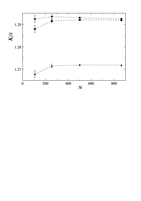
FIG. 1.: Reduced kinetic energy ${\cal K}/\epsilon$ vs. particle number $N$. The Trotter number is $P=8$, the temperature is $T=20$ K and the reduced density is $\rho/\rho^{*}=0.945$. $\rho^{*}\equiv{m}/\sigma^{3}=1.5479$ g cm^-3 is the characteristic density. The triangles are raw PIMC data, the squares are PIMC data plus finite-Trotter corrections (2) and the circles are PIMC data plus finite-Trotter and finite-size corrections (3). Error bars, when not shown, lie inside the symbols. Lines are guides for the eye.

Through this analysis we have concluded that for the kinetic energy of neon a simulation box with $108$ atoms and periodic boundary conditions is barely large enough to mimic the thermodynamic limit behaviour (i.e. the finite size corrections are of the order of the statistical error), as it can be seen in Fig. 1 where it’s shown how the finite-size corrections scheme works. The relative effect of finite-size and finite-Trotter corrections is well seen also in Fig. 2, where it is shown how the finite-Trotter corrections work. The small difference between the extrapolations at $P=\infty$ represents the size effect.

The results of our simulations are shown in Fig. 3: they are consistent with the experimental data [2] and confirm the validity of other PIMC simulations [2, 15].

In conclusion, the SCHA correction scheme gives an estimate on how large both the finite-size and the finite-Trotter effects are. It is indeed important to control how much the data are affected by the finiteness of the simulation box, especially for observables which possibly show a stronger $N$-dependence than the kinetic energy, such as the specific heat or the frequency moments, or for systems with larger quantum coupling.

We gratefully acknowledge useful discussions with P. Nielaba.

FIG. 2.: Reduced kinetic energy ${\cal K}/\epsilon$ vs. the inverse square of the Trotter number $P$. The simulation box contains $108$ particles, the temperature is $T=5$ K and the reduced density is $\rho/\rho^{*}=0.968$. The triangles are raw PIMC data, and the circles are PIMC data plus finite Trotter and finite size corrections (3). Error bars, when not shown, lie inside the symbols. The lines are fits of corresponding data.

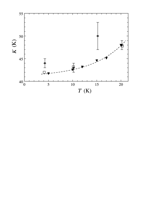
FIG. 3.: Kinetic energy ${\cal K}$ of solid neon vs. temperature $T$. The crosses are experimental data from [15], the open squares are PIMC simulations data from [15] and the triangles are our PIMC data with refined Trotter extrapolation. Error bars, when not shown, lie inside the symbols. The line is a guide for the eye.

REFERENCES

-
[1]
E-mail addresses: cuccoli@fi.infn.it, pedrolli@fi.infn.it,
macchi@fi.infn.it, tognetti@fi.infn.it, vaia@ieq.fi.cnr.it - [2] A. Cuccoli, A. Macchi, V. Tognetti and R. Vaia, Phys.Rev B 47, 14923 (1992).
- [3] R. Giachetti and V. Tognetti, Phys. Rev. Lett. 55, 912 (1985); Phys. Rev. B 33, 7646 (1986).
- [4] R. P. Feynman and H. Kleinert, Phys. Rev. A 34, 5080 (1996).
- [5] A. Cuccoli, R. Giachetti, V. Tognetti, R. Vaia and P. Verrucchi, J. Phys.: Condens. Matter 7, 7891 (1995).
- [6] S. Liu, G. K. Horton and E. R. Cowley, Phys. Lett. A 152, 79 (1991) and Phys. Rev. 44, 11714 (1991).
- [7] A. Cuccoli, A. Macchi, M. Neumann, V. Tognetti and R. Vaia, Phys.Rev B .45, 2088 (1992).
- [8] S. Liu, G.K. Horton, E.R. Cowley, A.R. McGurn, A.A. Maradudin and R.F. Wallis, Phys. Rev. 45, 9716 (1992).
- [9] D. Acocella, G. K. Horton and E. R. Cowley, Phys. Rev. B 51, 11406 (1995).
- [10] O. G. Peterson, D. N. Batchelder and R. O. Simmons, Phys. Rev. 150, 703 (1966).
- [11] M.A. Fradkin, S.X. Zheng and R.O. Simmons, Phys. Rev. 49, 3197 (1994).
- [12] D. Acocella, G. K. Horton and E. R. Cowley, Phys. Rev. Lett. 74, 4887 (1995).
- [13] M. H. Müser, P. Nielaba and K. Binder, Phys. Rev. B 51, 2723 (1995).
- [14] D. A. Peek, I. Fujita, M. C. Schmidt and R. O. Simmons, Phys. Rev. B 45, 9680 (1992).
- [15] D. N. Timms, A. C. Evans, M. Boninsegni, D. M. Ceperley, J. Mayers and R. O. Simmons, J. Phys.: Condens. Matter 8, 6665 (1996).
- [16] A. Cuccoli, A. Macchi, G. Pedrolli, V. Tognetti and R. Vaia, Phys. Rev. B 51, 12369 (1995).
- [17] A. Cuccoli, A. Macchi, G. Pedrolli, V. Tognetti and R. Vaia, unpublished.
- [18] M. Suzuki, Phys. Lett. A113, 299 (1985).
- [19] K. S. Schweizer, R. M. Stratt, D. Chandler and P. G. Wolynes, J. Chem Phys. 75, 1347 (1981).
- [20] T. R. Koehler, Phys. Rev. Lett. 17, 89 (1966).
- [21] N. S. Gillis, N. R. Werthamer and T. R. Koehler, Phys. Rev. 165, 951 (1968).
- [22] J. S. Brown, Proc. Phys. Soc. 89, 987 (1966).