Virial Expansions, Exclusion Statistics, and the Fractional Quantum Hall Effect

Abstract

We report on a study of virial expansions for interacting electrons in the lowest Landau level of a two-dimensional electron gas. For hard-core-model interactions, we derive analytic results valid at low temperatures and filling factors smaller than $1/3$ and comment on their relationship with virial expansions for exclusion statistics models. In the high temperature limit the virial coefficients reduce to those for a non-interacting electron system. For the first five virial coefficients, the crossover between low and high temperature limits has been studied numerically by using partition functions obtained from small system exact diagonalization calculations. Our results show that the exclusion statistics description of fractional Hall thermodynamics breaks down when the temperature exceeds a small fraction of the gap temperature.

I Introduction

The spectrum of the kinetic energy operator for a non-interacting electron in two dimensions in a perpendicular magnetic field consists of Landau levels with degeneracy and energy separation both proportional to the magnetic field strength $B$. In strong magnetic fields, the situation where all electrons can be accommodated within the lowest Landau level can be realized experimentally and affords an interesting archetype for strongly interacting electron systems. In such systems, the many-particle kinetic energy operator has a ground state degeneracy that grows exponentially with system size, frustrating attempts to describe the system by treating electron-electron interactions perturbatively. The physical properties of two-dimensional electron systems (2DES) have a corresponding richness, exhibiting a number of unusual properties including the fractional quantum Hall[1] effect (FQHE). The FQHE is related to discontinuities in the chemical potential[2] of a 2DES at zero temperature. Progress has been made in its theoretical understanding by a variety of approaches, including the use of variational many-electron wave functions,[3] the idenfication of model Hamiltonians[4, 5] for which the ground state may be determined analytically, and the introduction of artificial Chern-Simons magnetic flux quanta attached to each particle. [6, 7, 8, 9] In this article we discuss an initial attempt to address finite-temperature properties of 2DES’s in the FQHE regime using virial expansions.

Throughout this article we will restrict our attention to the situation where the energy separation between Landau levels ($\hbar\omega_{c}=\hbar eB/m^{*}c$) is much larger than the thermal energy $k_{B}T$ and assume that the electronic system is completely spin polarized so that we can truncate the Hilbert space to the lowest spin-polarized Landau level. In Section II we introduce appropriate definitions for cluster and virial expansion coefficients in this FQHE regime. Here we discuss the non-interacting electron limit and some exact properties of the virial expansion that follow from particle-hole symmetry within the lowest Landau level. For interacting electron systems, the non-interacting results for the virial coefficients are recovered in the high-temperature limit where $k_{B}T$ is much larger than the typical interaction energy per particle. All interaction-dependent results discussed in this article are for the case of hard-core-model electron-electron interactions. This model can be regarded as the ideal model of the fractional quantum Hall effect since the seminal variational wave functions of Laughlin are exact in this case.[4, 5] In Section III we derive exact results for the zero-temperature limit of the virial coefficients of the hard-core model. As we discuss there, the thermodynamics in this regime corresponds precisely to that of an exclusion statistics gas.[10] In order to study how the virial coefficients interpolate between their high-temperature and low-temperature limits, we have obtained numerically exact results for the temperature dependence of the five leading virial coefficients by calculating finite-size partition functions for small numbers of electrons. These results are presented and discussed in Section IV. In Section V we discuss the degree to which fractional quantum Hall behavior is reflected in the virial coefficients we have evaluated. Finally in Section VI we briefly summarize our results.

II Virial Expansions in the Lowest Landau Level

The virial expansion[11] can be derived from the expansion of the grand potential in powers of the fugacity, $z\equiv\exp(\mu/k_{B}T)$. This expansion is motivated in part by the fact that only its leading order term is non-zero for the classical non-interacting gas. Higher order terms in the expansion are due to quantum effects and interactions. The grand potential is extensive and for the two-dimensional case, the dimensionless coefficients of the virial expansion are conventionally defined by expressing the grand potential per unit area in units of $-k_{B}T/\lambda^{2}$ where $\lambda=(2\pi\hbar^{2}/m^{*}k_{B}T)^{1/2}$ is the thermal de Broglie wavelength and $m^{*}$ is the effective electronic mass. When the Hilbert space for a quantum system is truncated to the lowest Landau level, $m^{*}$ plays no role and a different normalization is more convenient. We develop our virial expansion for the FQHE regime by expanding the grand potential as follows:

$$\Omega(T,z)\equiv-k_{B}T\ln Z=-k_{B}TN_{\phi}\sum_{l=1}^{\infty}b_{l}(T)z^{l}$$ (1)

Here $N_{\phi}=AB/\Phi_{0}$ is the degeneracy of the Landau level, $A$ is the area of the system and $\Phi_{0}=hc/e$ is the electron magnetic flux quantum. The dimensionless coefficients $b_{l}(T)$ can be determined by expanding $\Omega(T,z)$ when this function is known analytically, by using perturbative cluster expansion approaches, or iteratively from canonical ensemble partition functions evaluated with successively larger finite number of electrons. We will refer to the coefficients $b_{l}(T)$ as cluster expansion coefficients. It follows from Eq. (1) that

$$\nu(T,z)=\sum_{l=1}^{\infty}lb_{l}(T)z^{l}$$ (2)

where $\nu(T,z)\equiv N(T,z)/N_{\phi}$ is the Landau level filling factor at finite temperature. The virial expansion is obtained from these two series by inverting Eq. (2) to obtain $z$ as a power series in $\nu$ and inserting the result in Eq. (1). The procedure is readily carried out to any finite order with the result that

$$\frac{-\Omega}{k_{B}TN_{\phi}}=\sum_{l=1}^{\infty}a_{l}(T)\nu^{l}$$ (3)

where $a_{l}(T)$ is $l^{\rm th}$ virial coefficient.

For 2DES’s in the fractional quantum Hall regime a number of other thermodynamic functions are of interest. We will comment extensively on the thermodynamic density of states:

$$g_{T} \equiv \frac{dN}{d\mu}=N_{\phi}\frac{z}{k_{B}T}\frac{d\nu}{dz}$$ (4)

$$= \frac{N_{\phi}}{k_{B}T}\sum_{l=1}^{\infty}g_{l}(T)\nu^{l};$$ (5)

the free energy

$$F=\Omega+Nk_{B}T\ln z=N_{\phi}k_{B}T\big{[}\nu\ln(\nu)+\sum_{l}f_{l}(T)\nu^{l}\big{]};$$ (6)

the entropy

$$S=\frac{-\partial F}{\partial T}=-N_{\phi}k_{B}[\nu\ln(\nu)+\sum_{l=1}^{\infty}\frac{d(Tf_{l}(T))}{dT}\nu^{l}];$$ (7)

and the heat capacity

$$C=T\frac{\partial S}{\partial T}=-N_{\phi}k_{B}\sum_{l=1}^{\infty}T\frac{d^{2}(Tf_{l}(T))}{dT^{2}}\nu^{l}.$$ (8)

Expressions for $a_{l}(T)$, $g_{l}(T)$, and $f_{l}(T)$ in terms of the cluster expansion parameters $b_{l}(T)$ are listed in Table I.

It is instructive to compute the coefficients of these expansions for the case of a non-interacting Fermi gas. We choose the zero of energy at the kinetic energy of particles in the lowest Landau level for convenience. Then the grand potential is given by

$$\Omega_{NI}=-N_{\phi}k_{B}T\ln(1+z).$$ (9)

Differentiating $\Omega_{NI}$ with respect to $\mu$ we recover the Fermi distribution function expression for the Landau level filling factor:

$$\nu=z/(1+z).$$ (10)

Expanding either Eq. (9) or Eq. (10) we identify the cluster expansion coefficients:

$$b_{l}^{NI}=(-1)^{l+1}/l.$$ (11)

Eq. (11) should be compared with the result for cluster expansion coefficients of quantum non-interacting Fermi gases in D space dimensions in zero magnetic field;[11] $b_{l}\propto(-1)^{l+1}l^{-1-D/2}$. As expected, in the strong field limit, Landau level degeneracy transforms thermodynamic properties of two-dimensional non-interacting electrons into those of a zero-dimensional system. However, interactions couple the orbital states within a Landau level and, as we shall see, the similarity to zero-dimensional systems is lost when interactions are important. We can invert Eq. (10) to express $z$ in terms of $\nu$. Substituting the result in Eq. (9) yields $\Omega_{NI}=N_{\phi}k_{B}T\ln(1-\nu)$ which can be expanded to identify the virial coefficients in the non-interacting case:

$$a_{l}^{NI}=1/l.$$ (12)

Similar elementary calculations yield $g_{T}^{NI}=N_{\phi}\nu(1-\nu)/k_{B}T$ and $F_{NI}=-TS_{NI}=N_{\phi}k_{B}T[\nu\ln\nu+(1-\nu)\ln(1-\nu)]$. It follows from these relations that $g_{1}^{NI}=1$ , $g_{2}^{NI}=-1$ and $g_{l}^{NI}=0$ for $l\geq 3$ and that $f_{1}^{NI}=-1$ and $f_{l}^{NI}=1/l(l-1)$ for $l\geq 2$. Note that the heat capacity vanishes and that the free energy is purely entropic in this model since the internal energy is zero at all temperatures.

In closing this section we remark on the particle-hole symmetry which exists in the lowest Landau level. It follows from this symmetry that[2] the chemical potentials at filling factors $\nu$ and $1-\nu$ are related by $\mu(\nu)+\mu(1-\nu)=2\epsilon_{0}$ where $\epsilon_{0}$ is the energy per-electron in the full Landau level state. $\epsilon_{0}$ is readily evaluated for any model electron-electron interaction; for the hard-core model discussed later in this article $\epsilon_{0}=4V_{1}$. When expressed in terms of the fugacity this relation takes the form $z(\nu)z(1-\nu)=\exp(2\epsilon_{0}/k_{B}T)$. The virial expansions discussed in this paper converge more rapidly at lower filling factors and higher temperatures. This particle-hole symmetry relation allow us to restrict our attention to the regime where $\nu<1/2$.

III Virial Expansion for the Infinite Hard Core Model

A convenient parameterization[4] of the interaction potential between a pair of electrons in the lowest Landau level results from the fact that there is only one possible relative motion state for each angular momentum.[2] Since isotropic interactions will be diagonal in relative angular momentum, the interaction Hamiltonian is completely specified by the interaction energy eigenvalue, $V_{l}$ associated with each relative angular momentum. (Only nonnegative relative angular momenta occur.) The $V_{l}$ parameters are known as Haldane pseudopotentials. For spin-polarized states only odd relative angular momentum states are permitted by the antisymmetry requirement on the many-fermion wave function. In the hard-core model (HCM) a pair of electrons interact with each other only when they are in the smallest possible relative angular momentum state, $l=1$, and the Hamiltonian is proportional to $V_{1}$. The Hamiltonian $H$ in this model can be written as

$$H=V_{1}\sum_{i<j}P_{ij}^{(1)}$$ (13)

Here $P_{ij}^{(1)}$ projects particles $i$ and $j$ onto a state of relative angular momentum $1$. The model is non-trivial since the projection operators for pairs with a common member do not commute. In this section we discuss the thermodynamics of the infinite hard-core model (IHCM) where $V_{1}\to\infty$. Since $V_{1}$ is the only energy scale in the hard-core model Hamiltonian, $V_{1}$ can be compared only with the thermal energy $k_{B}T$ and the results obtained for the virial coefficients here are $T\to 0$ limits of the general results for the hard-core model.

For $V_{1}\to\infty$ the only finite energy eigenstates of the hard-core model are the zero-energy eigenstates. The calculations in this section require only known[13] results for the degeneracy of the zero-energy eigenvalues as a function of $N_{\phi}$ and $N$. We briefly summarize one argument leading to this expression. For $N_{\phi}$ states in a Landau level, the symmetric gauge single-particle eigenstates are $\propto\xi^{m}\exp(-|\xi|^{2}/4)$ where we have adopted $\ell\equiv(A/2\pi N_{\phi})^{1/2}$ as the unit of length and $m=0,\ldots,N_{\phi}-1$. Here $\xi=x+iy$ is a complex coordinate. Zero energy many-body eigenstates of the HCM must have a symmetric-gauge many-body wave functions of the form[12, 2]

$$\Psi[\xi]=\left(\prod_{k=1}^{N}\exp(-|\xi_{k}|^{2}/4)\right)U[\xi]\left(\prod_{i<j}^{N}(\xi_{i}-\xi_{j})^{3}\right).$$ (14)

in order to avoid pairs in states of relative angular momentum one. $U[\xi]$ is any symmetric polynomial in each $\xi_{i}$ and can be regarded as a many-boson wave function. The maximum power to which each $\xi_{i}$ is raised in $\prod_{i<j}^{N}(\xi_{i}-\xi_{j})^{3}$ is $3(N-1)$ . Since the maximum possible power of a $\xi_{i}$ in $\Psi[\xi]$ is $N_{\phi}-1$ it follows that the number of zero energy eigenstates of the HCM, $g(N_{\phi},N)$ is equal to the number of $N$-boson states in which the bosons are allowed to occupy single-particle states with $0\leq m\leq N_{\phi}-1-3(N-1)$:

$$g(N_{\phi},N)={{N_{\phi}-2(N-1)}\choose N}.$$ (15)

$g(N_{\phi},N)$ can also[13] be regarded as the number of $N$ fermion states in which the fermions are allowed to occupy single-particle states with $0\leq m\leq N_{\phi}-1-2(N-1)$.

We now use Eq. (15) to determine the virial expansion coefficients of the IHCM. We obtain the expansion coefficients using two different approaches. First we obtain the coefficients using an iterative approach in which the cluster expansion coefficients are calculated from partition functions for systems containing different numbers of electrons. Our motivation here is to illustrate the approach used in the following section to treat the HCM at finite temperatures. The general relationship between the grand partition function ($Z$) and the canonical ensemble partition function for fixed particle number $N$ ($Q_{N}$) is

$$Z=\sum_{N=0}^{N_{\rm max}}z^{N}Q_{N}$$ (16)

For the infinite hard-core model the maximum $N$ for states in the Hilbert space is given by $N_{\rm max}=\left[(N_{\phi}+2)/3\right]$ and all states have zero energy so that $Q_{N}=g(N_{\phi},N)$. We define finite-size cluster coefficients $\tilde{b}_{l}$ by requiring Eq. (2) to hold for each finite value of $N_{\phi}$. Then

$$\langle N\rangle=\frac{\sum_{N=0}^{N_{\rm max}}NQ_{N}z^{N}}{Z}=N_{\phi}\sum_{N=0}^{\infty}N{\tilde{b}}_{N}z^{N}.$$ (17)

Multiplying both sides of Eq. (17) by $Z$ and equating coefficients of $z^{N}$ we find that

$$\tilde{b}_{N}=\frac{Q_{N}}{N_{\phi}}-\sum_{l=0}^{N-1}\frac{l}{N}{\tilde{b}}_{l}Q_{N-l}.$$ (18)

Using Eq. (18), knowledge of $Q_{l}$ for $l=1,\cdots,N$ is sufficient to evaluate $\tilde{b}_{l}$ for $l=1,\cdots,N$. Extrapolating to $N_{\phi}\to\infty$ gives the cluster coefficients $b_{l}$. For the IHCM $Q_{l}=g(N_{\phi},l)$ so this procedure is readily carried out. It is easy to show that the finite-size corrections to $\tilde{b}_{l}$ are $\propto N_{\phi}^{-1}$, facilitating the extrapolation to $N_{\phi}\to\infty$. The leading cluster coefficients obtained by this iterative procedure are listed in Table II.

Thermodynamic properties of the IHCM can be calculated analytically using several different approaches, one of which we outline below. For a finite $N_{\phi}$ the filling factor is related to the grand partition function by

$$\nu(N_{\phi},z)=\frac{z}{N_{\phi}}\frac{dZ/dz}{Z}.$$ (19)

Using the explicit expression for $Q_{N}=g(N_{\phi},N)$ it follows that for $N_{\phi}\to\infty$

$$\frac{d\nu}{d(\ln z)}=6\nu^{3}-5\nu^{2}+\nu$$ (20)

and hence that

$$z=\frac{\nu(1-2\nu)^{2}}{(1-3\nu)^{3}}.$$ (21)

Eq. (21) can be solved to express $\nu$ in terms of $z$:

$$\nu(z) = \frac{1}{3}-\frac{1}{54^{1/3}(4+27z)}$$ (23)

$$\ \ \times\left({\root 3 \of{(4+27z)^{2}-(27z(4+27z)^{3})^{1/2}}}+{\root 3 \of{(4+27z)^{2}+(27z(4+27z)^{3})^{1/2}}}\right)$$

The cluster expansion coefficients listed in Table II can be confirmed by expanding Eq. (23).

The virial expansion coefficients we have defined can be calculated from Eq. (21). The chemical potential as a function of filling factor is given by the equation:

$$\mu(\nu)=k_{B}T\ln\left(\frac{\nu(1-2\nu)^{2}}{(1-3\nu)^{3}}\right)$$ (24)

This equation shows explicitly that $\mu(\nu)$ diverges as $\nu\to 1/3$ in the IHCM. (For a finite $V_{1}$ HCM, $\mu$ has a finite jump discontinuity[14] at $\nu=1/3$.) Differentiating Eq. (24) with respect to $\nu$ we find an analytic expression for the thermodynamic density-of-states:

$$g_{T}=\frac{N_{\phi}}{k_{B}T}\nu(1-2\nu)(1-3\nu).$$ (25)

From Eq. (25) we see that for the IHCM $g_{1}^{IHC}=1$, $g_{2}^{IHC}=-5$, $g_{3}^{IHC}=6$ and $g_{l}^{IHC}=0$ for $l\geq 4$. It is remarkable that this expansion truncates at a finite order. The grand potential follows from Eq. (25) by using that $N=-\partial\Omega/\partial\mu$ and integrating over filling factors:

$$\Omega=-\int_{0}^{N}\frac{N^{\prime}}{g_{T}(N^{\prime})}dN^{\prime}=-k_{B}TN_{\phi}\ln\left(\frac{1-2\nu}{1-3\nu}\right).$$ (26)

From Eq. (26) we see that for the IHCM $a_{l}^{IHC}=(3^{l}-2^{l})/l$. This virial expansion converges only for $\nu<1/3$ as expected. Adding $\mu N$ to $\Omega$ we find that

$$F=-TS=N_{\phi}k_{B}T\big{[}\nu\ln\nu-(1-2\nu)\ln(1-2\nu)+(1-3\nu)\ln(1-3\nu)\big{]}.$$ (27)

so that $f_{1}^{IHC}=-1$ and $f_{l}^{IHC}=(3^{l}-2^{l})/l(l-1)$ for $l\geq 2$. As for the non-interacting electron model the free energy is purely entropic because all states in the Hilbert space have zero energy. The expression for the entropy in Eq. (27) can be obtained from large number approximations for $g(N_{\phi},N)$ and is the starting point for an alternate canonical ensemble derivation of the above expressions.

It is worth commenting on the relationship between the statistical mechanics of the IHCM and the statistical mechanics of exclusion statistics gases.[10] The exclusion statistics concept was first proposed by Haldane, motivated in part by interest in the statistics of the fractionally charged quasiparticles[3] of the fractional quantum Hall effect.[15] In a system with exclusion statistics parameter $g$ the number of states available to an added electron, appropriately defined, is decreased by $g$ units for each added particle. With this definition, it is readily shown that for the hard-core model the fractionally charged quasiholes[16] of the $\nu=1/3$ state in the fractional quantum Hall effect, present in low-energy states for $\nu<1/3$, satisfy exclusion statistics with statistics parameter $g=1/3$. On the other hand Eq. (21) can be recognized as the equation satisfied by the occupation number distribution function[17, 18, 19, 20, 21] of a fractional statistics gas with statistics parameter $g=3$. The difference between these statistics parameters is readily understood from the equivalence between the number of zero-energy states in the IHCM and the number of many-boson states in a Hilbert space with $N_{\phi}-3(N-1)-1$ single-particle levels. Eq. (21) is identical to the corresponding relation for a $g=3$ exclusion statistics gas because $3$ single-particle states are lost for each added electron. On the other hand, when the zero-energy states of the hard-core model are described[13] in the language of fractionally charged quasiholes, the number of particles is $N_{qh}=N_{\phi}-3(N-1)-1$ and the number of available states is $N$. Quasiholes are added at fixed $N_{\phi}$ by decreasing $N$ so that the number of states is decreased by one for each three added particles giving exclusion statistics parameter $g=1/3$. The fact that IHCM is equivalent to both a $g=1/3$ exclusion statistics gas of quasiholes and a $g=3$ exclusion statistics gas of electrons is related to the exclusion statistics particle-hole dualities noted by Nayak and Wilczek[18]. At higher temperatures the description in terms of quasiholes is no longer useful, hence for our purposes it is more useful to regard the zero-temperature limit of the HCM as a $g=3$ exclusion statistics electron system.

The results obtained here for the IHCM in which $V_{1}\to\infty$ can be generalized to models where infinite repulsion occurs in all relative motion states with odd relative angular momentum less than or equal to $m$. In this case the grand partition function is

$$Z^{(m)}=\sum_{k=0}^{N_{\rm max}^{(m)}}{{mN_{\rm max}^{(m)}-(m-1)k}\choose k}z^{k}$$ (28)

where $N_{\rm max}^{(m)}\equiv[(N_{\phi}+m-1)/m]$. These models correspond generally to $g=m$ fractional statistics gases and the results described above have simple correspondences. For example,

$$z=\frac{\nu(1-(m-1)\nu)^{m-1}}{(1-m\nu)^{m}},$$ (29)

$$\mu=k_{B}T\ln\left(\frac{\nu(1-(m-1)\nu)^{m-1}}{(1-m\nu)^{m}}\right),$$ (30)

and

$$\Omega^{(m)}=-k_{B}TN_{\phi}\ln\left(\frac{1-(m-1)\nu}{1-m\nu}\right).$$ (31)

The chemical potential now diverges at $T=0$ for $\nu\to\frac{1}{m}$.

IV Numerical results at finite T

In this section we evaluate the expansion coefficients at finite temperatures assuming HCM electron-electron interactions. The first two cluster coefficients can be calculated analytically giving $b_{1}(T)=1$ and $b_{2}(T)=-2.5+2\exp(-\beta V_{1})$ where $\beta\equiv 1/k_{B}T$. This result for $b_{2}(T)$ follows from analytic results for the complete many-particle energy spectrum and the canonical ensemble partition function for a two electron problem in a degenerate Landau level. To proceed further we numerically diagonalize the HCM Hamiltonian for finite systems with up to five electrons and three values of $N_{\phi}=17,19,21$. The first five cluster coefficients are then evaluated iteratively by using Eq. (18) and extrapolating to the limit $N_{\phi}\to\infty$. The leading finite size corrections to the virial coefficients are proportional to $N_{\phi}^{-1}$, as for the infinite hard-core model and the extrapolation to $N_{\phi}\to\infty$ can be carried out with some confidence. The other expansion coefficients can be obtained using the relations given in Table I. The results are summarized in Figs. 1 - 4. We note that the crossover between low and high temperature limits of the cluster coefficients begins for $k_{B}T\sim 0.1V_{1}$. The chemical potential discontinuity at $\nu=1/3$ in the HCM is[14] $\sim V_{1}$; it follows that deviations from exclusion model thermodynamics in the fractional quantum Hall effect start to become important at temperatures well below the gap temperature. We also note that although the virial coefficients, $a_{l}(T)$, are positive for $T=0$ ($a_{l}=(3^{l}-2^{l})/l$) and $T\to\infty$ ($a_{l}=1/l$) limits, they do become negative at intermediate temperatures. In addition, the higher $l$ coefficients in the virial expansion of the thermodynamic density of states, which vanish in both high temperature and low temperature limits, are comparable to the $l=2$ and $l=3$ coefficients at intermediate temperatures.

We can compare some of these results with analytic many-body perturbation theory results[22] for leading terms in the expansion of the grand potential in powers of $\beta V_{1}$. It follows from that approach that at high temperatures

$$f_{2}(T) = f_{2}^{NI}+2\beta V_{1}-(\beta V_{1})^{2}+(\beta V_{1})^{3}/3+O(\beta V_{1})^{4},$$ (32)

$$f_{3}(T) = f_{3}^{NI}+2(\beta V_{1})^{2}-140(\beta V_{1})^{3}/81+O(\beta V_{1})^{4},$$ (33)

$$f_{4}(T) = f_{4}^{NI}-(\beta V_{1})^{2}+95(\beta V_{1})^{3}/27+O(\beta V_{1})^{4},$$ (34)

$$f_{5}(T) = f_{5}^{NI}-86(\beta V_{1})^{3}/27+O(\beta V_{1})^{4}.$$ (35)

Note that the leading correction to $f_{2}$ is linear in $\beta V_{1}$ while the leading correction to $f_{3}$ is quadratic in $\beta V_{1}$. These corrections can be extracted from our numerical results and they are plotted in Fig. 5. For $l=3$ some discrepancy between the analytic result is visible at the left hand side of this log-log plot. We attribute this discrepancy to errors associated with the extrapolation of the numerical results to the thermodynamic limit. (The discrepancy for $f_{3}$ at $\beta V_{1}=e^{-4}$ is $\sim 0.0005$ compared to the $T\to\infty$ value $f_{3}^{NI}=1/6$.) For $l=4$ and $l=5$ finite size effects are larger so we should expect the remnant finite-size error to be larger. On the other hand, the high $T$ corrections to $f_{l}$ are smaller at a given value of $\beta V_{1}$. For this reason we have been unable to establish agreement between our numerical results and the coefficients of the leading high temperature correction terms in these cases.

At low temperatures leading corrections to $f$-coefficients show activated behavior, with the activation energy decreasing slowly with increasing $l$. In the next section we will attempt to estimate some thermodynamic properties using information from this virial expansion. For $l>5$ we know only the $T=0$ and $T=\infty$ limits of the coefficients; this motivates testing the reliability of simple formulas for interpolating between the two limits. For example, we have examined approximating the temperature dependence of the $f$-coefficients by the formula

$$f_{l}(T)=f_{l}^{IHC}+(f_{l}^{NI}-f_{l}^{IHC})\exp(-\lambda_{l}\beta V_{1})$$ (36)

where the $\lambda_{l}$ are fitting parameters. This form is exact for $l=1$ and $l=2$ with $\lambda_{1}=0$ and $\lambda_{2}=1$. The fact that the high temperature corrections to the non-interacting Fermi gas values are not captured by these formulas provides a cautionary indication that this approach might not be wholly successful. Using a least squares criterion to fit $f_{3}(T)$, $f_{4}(T)$, and $f_{5}(T)$, we find the optimal values of $\lambda_{3}=0.5987$, $\lambda_{4}=0.5181$, and $\lambda_{5}=0.4870$. We note that truncating the virial expansion at fifth order introduces a relative error of at most 1% for the free energy evaluated at $\nu\leq 1/6$ and zero temperature. At higher temperatures the virial expansion will converge more rapidly. Nevertheless, at low temperatures and filling factors close to $\nu=1/3$ a truncated virial expansion will never suffice. In the next section we discuss using interpolation formulas like Eq. (36) to continue the expansion to higher orders.

V Thermodynamic Properties From the Virial Expansion

In this section we use information from our virial expansion study to estimate some thermodynamic properties in the quantum Hall regime. Except where noted, the expansion is carried out to convergence. At low temperatures this frequently requires virial coefficients with indices larger than $l=5$. In these cases we have approximated $f_{l}(T)$ using Eq. (36) with $\lambda_{l}$ extrapolated[23] from the values obtained by fitting, as described above, to larger values of $l$. In Fig. 6 the entropy is plotted as a function of filling factor. The $T=0$ and $T=\infty$ curves show exclusion statistics and free particle thermodynamics respectively. The temperature dependence of the entropy is strongest at $\nu=1/3$ where the large non-interacting electron value is reduced to zero at $T=0$ because the Laughlin state[3] is the only thermally accessible state. The approximate entropy we obtain using the procedures described above has unphysical negative values at low temperatures for $\nu>1/3$. The naive extrapolation procedure we use at large $l$ is not sufficiently subtle to capture the chemical potential jump and entropy cusp which occur at $T=0$. The specific heat is plotted over the same filling factor range in Fig. 7. Note that the specific heat would be strictly zero without electron-electron interactions. In the fractional quantum Hall effect regime electrons don’t move faster as they heat up; instead they are more likely to occupy states in which particle positions are less strongly correlated and the interaction energy increases.

The thermodynamic density of states is plotted in Fig. 8. This is one of the most experimentally accessible thermodynamic properties of two-dimensional electron systems, thanks to clever capacitative coupling schemes[24] which take advantage of the possibility of making separate contact to nearby two-dimensional electron layers. In this case the expansion truncates at a finite order in both $T=0$ and $T\to\infty$ limits and better convergence properties allow us to use only the five explicitly calculated expansion coefficients for the calculation. The accuracy of this truncated expansion is indicated by comparing with results obtained when only four terms are used in the expansion. The vanishing thermodynamic density of states at zero temperature for $\nu=1/3$ is the incompressibility property which is central to the fractional quantum Hall effect. We find that this basic thermodynamic signature of the fractional quantum Hall effect is completely absent when $T$ reaches half of the gap temperature.

VI Summary

We have examined the virial expansion for a 2D electron gas in the fractional quantum Hall regime using a hard-core model for electron-electron interactions. The expansion coefficients depend only on the ratio of the hard-core interaction strength $V_{1}$ to the thermal energy $k_{B}T$. They may be evaluated analytically in both the non-interacting high-temperature limit and in the zero-temperature limit where the thermodynamics is equivalent to that of an exclusion statistics gas. We have evaluated the five leading expansion coefficients at intermediate temperatures numerically by using an exact diagonalization approach to evaluate the canonical ensemble partition function for up to N=5 particles in finite systems and extrapolating to the thermodynamic limit. We have used our results to estimate finite temperature properties of fractional quantum Hall systems and find that the characteristic behavior of the fractional quantum Hall effect disappears at temperatures well below the fractional quantum Hall gap temperature.

This work was supported by the National Science Foundation under grant DMR-9416906. The authors are grateful to Lian Zheng for advice on his high-temperature expansion results.

TABLE I.: Relations between the first five cluster coefficients and the other expansion parameters.

$l$	$a_{l}$	$f_{l}$	$g_{l}$
1	$b_{1}$	$-b_{1}$	$b_{1}$
2	$-b_{2}$	$-b_{2}$	$2b_{2}$
3	$-2b_{3}+4b_{2}^{2}$	$-b_{3}+2b_{2}^{2}$	$6b_{3}-8b_{2}^{2}$
4	$-3b_{4}+18b_{2}b_{3}-20b_{2}^{3}$	$-b_{4}+6b_{2}b_{3}-20b_{2}^{3}/3$	$12b_{4}-48b_{2}b_{3}+40b_{2}^{3}$
5	$-4b_{5}-144b_{2}^{2}b_{3}$	$-b_{5}-36b_{2}^{2}b_{3}$	$20b_{5}+360b_{2}^{2}b_{3}$
	$+32b_{2}b_{4}+18b_{3}^{2}+112b_{2}^{4}$	$+8b_{2}b_{4}+9b_{3}^{2}/2+28b_{2}^{4}$	$-112b_{2}b_{4}-54b_{3}^{2}-224b_{2}^{4}$

TABLE II.: Numerical values of the first five expansion coefficients in the IHCM limit.

$l$	$b_{l}^{IHC}$	$a_{l}^{IHC}$	$f_{l}^{IHC}$	$g_{l}^{IHC}$
1	1	1	$-1$	1
2	$-5/2$	5/2	5/2	$-5$
3	28/3	19/3	19/6	6
4	$-165/4$	65/4	65/12	0
5	1001/5	211/5	211/20	0

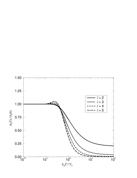
FIG. 1.: The temperature dependence of the first five cluster coefficients. ($b_{1}\equiv 1$ and it is not shown.)

FIG. 2.: The temperature dependence of the first five virial coefficients. ($a_{1}\equiv 1$ and it is not shown.)

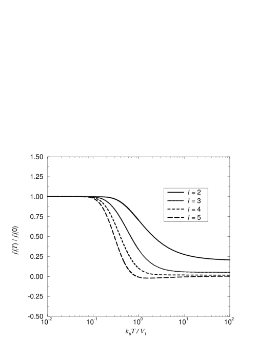
FIG. 3.: The temperature dependence of the first five $f$-coefficients. ($f_{1}\equiv-1$ and it is not shown.)

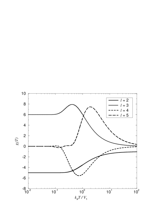
FIG. 4.: The temperature dependence of the first five $g$-coefficients. ($g_{1}\equiv 1$ and it is not shown.)

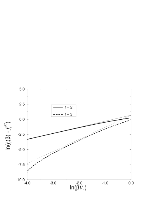
FIG. 5.: Leading order high-temperature corrections to the non-interacting Fermi gas values for $f_{2}(T)$ and $f_{3}(T)$. The thin lines correspond to the analytical leading order corrections.

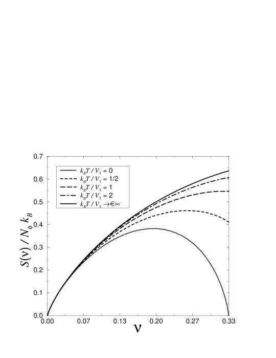
FIG. 6.: Entropy of a HCM gas vs. filling factor at different temperatures.

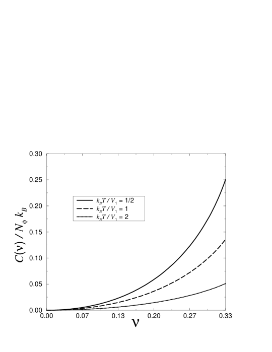
FIG. 7.: Heat Capacity of a HCM gas vs. filling factor at different temperatures.

FIG. 8.: Thermodynamic Density of States of a HCM gas vs. filling factor at different temperatures. The thick and thin lines correspond to the expansion truncated at fifth and forth orders, respectively.

REFERENCES

- [1] The Quantum Hall Effect, edited by R. E. Prange and S. M. Girvin (Springer-Verlag, New York, 1990); The Quantum Hall Effect: A Perspective, edited by A. H. MacDonald (Jaca Books, Milano, 1989); T. Chakraborty, P. Pietiläinen, The Quantum Hall Effects, (Springer-Verlag, Berlin, 1995); Quantum Hall Effect, edited by M. Stone (World Scientific, Singapore, New Jersey, London, Hong Kong, 1992).
- [2] See for example A. H. MacDonald in Mesoscopic Quantum Physics, edited by E. Akkermans, G. Montambaux, J.-L. Pichard, and J. Zinn-Justin (Elsevier, Amsterdam, 1995).
- [3] R.B. Laughlin, Phys. Rev. Lett. 51, 605 (1983).
- [4] See F. D. M. Haldane in The Quantum Hall Effect , edited by R. E. Prange and S. M. Girvin (Springer-Verlag, New York, Berlin, Heidelberg, Tokyo, 1990) and work cited therin.
- [5] S.A. Trugman and S. Kivelson, Phys. Rev. B 31, 5280 (1985).
- [6] J.K. Jain, Phys. Rev. Lett. 63, 199 (1989); Phys. Rev. B 40, 8079 (1989); ibid 41, 7653 (1990).
- [7] B.I. Halperin, P.A. Lee, and N. Read, Phys. Rev. B 47, 7312 (1993) and work cited therein.
- [8] S. Kivelson, D.H. Lee, and S.C. Zhang, Phys. Rev. B 46, 2223 (1992) and work cited therein.
- [9] Ana Lopez and Eduardo Fradkin, Phys. Rev. B 47, 7080 (1993).
- [10] F.D.M. Haldane, Phys. Rev. Lett. 67, 937 (1991). Y.-S. Wu, Phys. Rev. Lett. 73, 922 (1994); A.K. Rajagopal, Phys. Rev. Lett. 74, 1048 (1995); C. Nayak and F. Wilczek, Phys. Rev. Lett. 73, 2740 (1994); M.V.N. Murthy, and R. Shankar, Phys. Rev. Lett. 73, 3331 (1995); Wu-Pei Su, Yong-Shi Wu and Jian Yang, Phys. Rev. Lett. 77, 3423 (1996); S.B. Isakov, G.S. Canright, and M.D. Johnson, preprint (1996).
- [11] See for example, Kerson Huang, Statistical Mechanics (John Wiley & Sons, New York, 1987)
- [12] S. M. Girvin and Terrence Jach, Phys. Rev. B 29, 5617 (1984).
- [13] A. H. MacDonald, Helv. Phys. Acta, 65, 133 (1992) and work cited therein.
- [14] Claudius Gros and A.H. MacDonald, Phys. Rev. B 42, 9514 (1990).
- [15] B.I. Halperin, Phys. Rev. Lett. 52, 1583 (1984); 52, 2390(E) (1984).
- [16] Fractionally charged quasiparticles of the state, present in low-energy states for satisfy exclusion statistics with statistics parameter : S.He, X.C. Xie, and F.C. Zhang, Phys. Rev. Lett. 68, 3460 (1992); J. Yang, Phys. Rev. B 50, 11196 (1994); M.D. Johnson and G.S. Canright, Phys. Rev. B 49, 2947 (1994).
- [17] Y.-S. Wu, Phys. Rev. Lett. 73, 922 (1994).
- [18] C. Nayak and F. Wilczek, Phys. Rev. Lett. 73, 2740 (1994).
- [19] Anthony Chan and A.H. MacDonald in Physics of Quantum Solids of Electrons, edited by S.T. Chui (International Press, Hong Kong, 1994) p. 82.
- [20] A.K. Rajagopal, Phys. Rev. Lett. 74, 1048 (1995); A.K. Rajagopal and S. Teitler, Physica 147A, 627 (1988).
- [21] Virial expansions for exclusion statistics systems have been considered by M.V.N. Murthy, and R. Shankar, Phys. Rev. Lett. 73, 3331 (1995) and related to earlier work on virial expansions for anyon statistics models: D.P. Arovas, J.R. Schrieffer, F. Wilczek, and A. Zee, Nucl. Phys. B251, 117 (1985).
- [22] Lian Zheng and A.H. MacDonald, Surf. Sci. 305, 101 (1994) and to be published.
- [23] The extrapolation formula we use is with coefficients obtained using the least squares approximation for the known values of , , , and : , , , .
- [24] J.P. Eisenstein, L.N. Pfeiffer, and K.W. West, Phys. Rev. B 50, 1760 (1994); J.P. Eisenstein, L.N. Pfeiffer, and K.W. West, Phys. Rev. Lett. 68, 674 (1992).