Disorder in Two Dimensional Josephson Junctions

Abstract

An effective free energy of a two dimensional (i.e. large area) Josephson Junctions is derived, allowing for thermal fluctuations, for random magnetic fields and for external currents. We show by using replica symmetry breaking methods, that the junction has four distinct phases: disordered, Josephson ordered, a glass phase and a coexisting Josephson order with the glass phase. Near the coexistence to glass transition at $s=1/2$ the critical current is $\sim(\mbox{area})^{-s+1/2}$ where $s$ is a measure of disorder. Our results may account for junction ordering at temperatures well below the critical temperature of the bulk in high $T_{c}$ trilayer junctions.

I Introduction

Recent advances in fabrication of Josephson junctions (JJ) have led to junctions with large area, i.e. the junction length L (in either direction in the junction plane) is much larger than $\lambda$, the magnetic penetration length in the bulk superconductors. Experimental studies of trilayer junctions like [1] $YBa_{2}Cu_{3}O_{x}/PrBa_{2}Cu_{3}O_{x}/YBa_{2}Cu_{3}O_{x}$ (YBCO junction) or like [2] $Bi_{2}Sr_{2}CaCu_{2}O_{8}/Bi_{2}Sr_{2}Ca_{7}Cu_{8}O_{20}/Bi_{2}Sr_{2}CaCu_{2}O_{8}$ (BSSCO junction) have shown anomalies in the temperature dependence of the critical current $I_{c}$. In particular in the YBCO junction [1] with area of $50\mu m^{2}$ a zero resistance state was achieved only below $~{}50K$, although the $YBa_{2}Cu_{3}O_{x}$ layers were superconducting already at $T_{c}\approx 85K$. More recent data on similar YBCO junctions [3, 4, 5] with junction areas of $10^{2}-10^{4}\mu m^{2}$ show a measurable $I_{c}$ only at $20-60K$ below $T_{c}$ of the superconducting layers. An even larger junction [6] of area $\approx 10^{5}\mu m^{2}$ shows a well defined gap structure in the $I-V$ curve while a critical current is not observed. In the BSCCO junction [2] a supercurrent through the junction could not be observed above $30K$, although the $Bi_{2}Sr_{2}CaCu_{2}O_{8}$ layer remained superconducting up to $T_{c}\approx 80K$.

These remarkable observations are significant both as basic phenomena and for junction applications. In particular, these data raise the question of whether thermal fluctuations or disorder can significantly lower the ordering temperature of two dimensional (2D) junctions.

We note that for both YBCO and BSCCO junctions typically $\lambda\approx 0.2\mu m$ at low temperatures where the junctions order, so that the junctions above are 2D in the sense that disorder and spatial fluctuations on the scale of $\lambda$ can be important. The qualitative effect of these fluctuations depends on the Josephson length $\lambda_{J}$ ($\lambda_{J}>\lambda$) which is the width of a Josephson vortex (see section II). For $\lambda<L<\lambda_{J}$ junction parameters are renormalized and become L dependent, while more significant renormalizations which correspond to 2D phase transitions occur in the regime $\lambda_{J}<L$. From magnetic field dependence [4] and $L$ dependence [7] of $I_{c}$, junctions with $\lambda_{J}<L$ can be realized. The studied junctions are 2D also in the sense the thermal fluctuations at temperature T do not lead to uniform large phase fluctuations, i.e. $\phi_{0}I_{c}/2c<T$, a condition valid for the relevant data (see section V); $\phi_{0}=hc/2e$ is the flux quantum.

The energy of a 2D junction, in terms of the Josephson phase $\varphi_{J}(x,y)$ where $(x,y)$ are coordinates in the junction plane, was derived by Josephson [8]. It has the form

$${\cal F}_{0}=\int dxdy(\frac{\tau}{16\pi}({\bf\nabla}\phi_{J})^{2}+\frac{E_{J}}{\lambda^{2}}(1-\cos\varphi_{J}))$$ (1)

where $E_{J}$ is the Josephson coupling energy in area $\lambda^{2}$.

Equation (1) was derived [8] on a mean field level, i.e. only its value at minimum is relevant. It was shown, however, (see Ref.[9] and Appendix A) that Eq. (1) is valid in a much more general sense, i.e. it describes thermal fluctuations of $\varphi_{J}(x,y)$ so that a partition function at temperature $T(<T_{c})$

$$Z=\int{\cal D}\phi_{J}\exp\{-{\cal F}_{0}[\varphi_{J}(x,y)]/T\}$$ (2)

is valid.

Equation (2) implies a Berezinskii-Kosterlitz-Thouless type phase transition [10] at a temperature $T_{J}\approx\tau$ so that at $T>T_{J}$ the phase $\phi_{J}$ is disordered, i.e. the $\cos\phi_{J}$ correlations decay as a power law while at $T<T_{J}\;\cos\phi_{J}$ achieves long range order. For the clean system, however, $T_{J}\approx\tau$ is too close to $T_{c}$ for either separating bulk from junction fluctuations or for accounting for the experimental data [9]. A consistent description of this transition, as shown in the present work, can be achieved by allowing for disorder at the junction, a disorder which reduces $T_{J}$ considerably.

Equation (1) with disorder is related to a Coulomb gas and surface roughening models which were studied by replica and renormalization group (RG) methods [11, 12]. We find, however, that RG generates a nonlinear coupling between replicas and therefore standard replica symmetric RG methods are not sufficient. In fact, related systems [13, 14] were shown to be unstable towards replica symmetry breaking (RSB).

In our system we find a competition between long range Josephson type ordering and formation of a glass type RSB phase. The phase diagram has four phases: a disordered phase, Josephson phase (i.e. ordered with finite renormalized Josephson coupling), a glass phase and a coexistence phase. The coexistence phase is unusual in that it has Josephson type long range order coexisting with a glass order parameter. This phase is distinguished from the usual ordered phase, presumably, by long relaxation phenomena typical to glasses [15].

In the disordered and glass phases fluctuations reduce the critical current by a power of the junction area, while in the Josephson and coexistence phases the fluctuation effect saturates when the $(\mbox{area})^{1/2}$ is larger than either the Josephson length (in the Josephson phase) or larger than both the Josephson length and a glass correlation length (in the coexistence phase). These predictions can serve to identify these phases. We show that a transition between the glass phase and the coexistence phase can occur well below the critical temperature $T_{c}$ of the bulk, a result which may account for the experimental data on trilayer junctions [1, 2, 3, 4, 5].

In section II we define the model and study the pure case. In section III we study the system with random magnetic fields due to, e.g., quenched flux loops in the bulk and show that RG generates a coupling between different replicas. The system with disorder is solved by the method of one-step RSB [13, 16] in section IV. Appendix A derives the free energy of a 2D junction. In particular, Appendix A2 allows for space dependent external currents, a situation which, as far as we know, was not studied previously. Appendix B extends the one step solution of section IV to the general hierarchical case, showing that they are equivalent.

II Thermal effects

Appendices A.1-A.4 derive the effective free energy of a 2D junction, in presence of an external current $j^{ex}(x,y)$, for the geometry shown in Fig. 1. The presence of $j^{ex}(x,y)$ dictates that the relevant thermodynamic function is a Gibbs free energy, Eq. (A11) which for the junction becomes (Eqs. (A29,A50))

$${\cal G}_{J}\{\phi_{J}\}={\cal F}_{0}\{\phi_{J}\}-(\phi_{0}/2\pi c)\int dx\,dy\,j^{ex}(x,y)\varphi_{J}(x,y)$$ (3)

where ${\cal F}_{0}$ is given by Eq. (1). The cosine term is the Josephson tunneling [8] valid for weak tunneling $E_{J}<<\tau$ and $\tau$ is found in two cases (Eqs. (A27,A46)): Case I of long superconducting banks $W_{1},W_{2}>>\lambda$ and case II of short banks, $W_{1},W_{2}<<\lambda$,

$$\tau=\left\{\begin{array}[]{ll}\frac{\phi_{0}^{2}}{4\pi^{2}\lambda}&\mbox{\hskip 85.35826ptcase I: $W_{1},W_{2}>>\lambda$}\\ \\ \frac{\phi_{0}^{2}}{2\pi^{2}}\frac{W_{1}W_{2}}{\lambda_{1}^{2}W_{2}+\lambda_{2}^{2}W_{1}}&\mbox{\hskip 85.35826ptcase II: $W_{1},W_{2}<<\lambda$}\end{array}\right.$$ (4)

Note that in case II the derivation allows for an asymmetric junction with different penetration lengths $\lambda_{1},\lambda_{2}$ and different lengths $W_{1},W_{2}$.

It is of interest to note that $j^{ex}$ breaks the symmetry $\varphi_{J}\rightarrow\varphi_{J}+2\pi$, i.e. the external current distinguishes between different minima of the cosine term in Eq. (1). For a uniform $j^{ex}$ the Gibbs term reduces to the previously known form [17].

Appendices (A1-A4) present detailed derivation of Eq. (3). This derivation is essential for the following reasons: (i) It shows that the fluctuations of $\varphi_{J}$ decouple from phase fluctuations in the bulk, (excluding flux loops in the bulk which are introduced in section III). Thus Eq. (3) is valid below the fluctuation (or Ginzburg) region around $T_{c}$. (ii) It shows that Eq. (3) is valid for all configurations of $\varphi_{J}$ and not just those which solve the mean field equation.

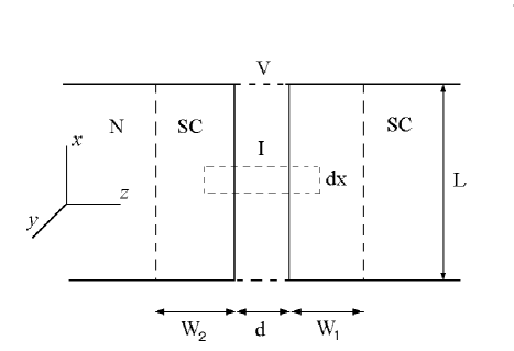
FIG. 1.: Geometry of the 2D Josephson junction. The various components are superconductors (S), insulating barrier (I), normal metal (N) for the external leads and vacuum (V). The dashed rectangle serves to derive boundary conditions in Appendix A 1.

It is instructive to consider the mean field equation $\delta G_{J}/\delta\varphi_{J}=0$, i.e.

$$\frac{E_{J}}{\lambda^{2}}\sin\varphi_{J}=\frac{\tau}{8\pi}{\bf\nabla}^{2}\varphi_{J}+\frac{\phi_{0}}{2\pi c}j^{ex}$$ (5)

This equation can also be derived by equating the current $j_{z}=(-c/4\pi\lambda^{2})A_{z}^{\prime}$ at $z=d/2$ (given, e.g. in case I by Eqs. (A20, A26)] with the Josephson tunneling current $j_{J}=(2\pi c/\phi_{0})(E_{J}/\lambda^{2})\sin\varphi_{J}$. Eq. (5), however, is not on a level of conservation law or a boundary condition since configurations which do not satisfy Eq. (5) are allowed in the partition sum. More generally, Eq. (5) is satisfied only after thermal average $\langle\delta G_{J}/\delta\varphi_{J}\rangle=0$. An equivalent way of studying thermal averages is to add to Eq. (5) time dependent dissipative and random force terms. The time average, which includes configurations which do not satisfy Eq. (5), is by the ergodic hypothesis equivalent to the partition sum, i.e. a functional integral over $\varphi_{J}$ with the weight $\exp[-G_{J}/T]$.

Eq. (1) is the well known 2D sine-Gordon system [10] which for $j^{ex}=0$ exhibits a phase transition. Since renormalization group (RG) proceeds by integrating out rapid variations in $\varphi_{J}$, $j^{ex}\neq 0$ is not effective if it is slowly varying (e.g. as in case II).

RG integrates fluctuations of $\varphi_{J}$ with wavelengths between $\xi$ and $\xi+\,d\xi$, the initial scale being $\lambda$. The parameters $t=T/\tau$ and $u=E_{J}/T$ are renormalized, to second order in $u$, via [10]

$$du/u = 2(1-t)\,d\xi/\xi$$ (6)

$$dt = 2\gamma^{2}u^{2}t^{3}\,d\xi/\xi$$ (7)

where $\gamma$ is of order 1 (depending on the cutoff smoothing procedure). Eq. (7) defines a phase transition at $1/t=1-\gamma u$. Note, however, that $\tau$ itself is temperature dependent since $\lambda(T)=\lambda^{\prime}(1-T/T_{c}^{0})^{-1/2}$, where $T_{c}^{0}$ is the mean field temperature of the bulk. Thus the solution of $\tau(T)/T=1-\gamma E_{J}/T$ defines a transition temperature $T_{J}$ which is below $T_{c}^{0}$. However, $T_{J}$ is too close to $T_{c}^{0}$ and is in fact within the Ginzburg fluctuation region around $T_{c}^{0}$. To see this, consider a complex order parameter $\psi=|\psi|\exp(i\varphi)$ with a free energy of the form

$\displaystyle{\cal F}=\int d^{3}r[a|\psi|^{2}+b|\psi|^{4}+a\xi^{2}|{\bf\nabla}\psi|^{2}]$

The Ginzburg criterion equates fluctuations with $b=0$, i.e. $\langle\delta\psi^{2}\rangle\approx T/a\xi^{3}$ with $|\psi|^{2}(=|a|/2b)$ in the ordered phase. Since $|{\bf\nabla}\psi|^{2}\approx|\psi|^{2}({\bf\nabla}\varphi)^{2}$ Eq. (A15) identifies $a\xi^{2}|\psi|^{2}=(\phi_{0}/2\pi\lambda)^{2}/8\pi$, so that the Ginzburg temperature is

$$T^{Ginz}=a\xi^{3}|\psi|^{2}=\xi(\phi_{0}/2\pi\lambda)^{2}/8\pi.$$ (8)

Since $\xi<\lambda,W$ in both cases I and II, $T^{Ginz}<T_{J}$. The neglect of flux loop fluctuations, as assumed in appendices A3, A4 is therefore not justified at $T_{J}$. Thus the relevant range of temperatures for the free energy Eqs. (1,3) is $T\ll T^{Ginz}<\tau$, i.e. $t\ll 1$.

The RG Eqs. (7) can, however, be used in the range $T<T_{J}$ to study fluctuation effects in the ordered region. Excluding a narrow interval near $T_{J}$ where $|\tau/T-1|<\gamma E_{J}/T<<1$ renormalization of $t$ can be neglected and integration of Eq. (7) yields a renormalized Josephson coupling $E_{J}^{R}=E_{J}(\xi/\lambda)^{2(1-t)}$. Scaling stops at the Josephson length $\lambda_{J}$ at which the coupling becomes strong, $E_{J}^{R}\approx\tau/8\pi$ (the $8\pi$ is chosen so that $\lambda_{J}=\lambda_{J}^{0}$ at $T=0$, where $\lambda_{J}^{0}$ is the conventional Josephson length). Thus $\lambda_{J}=\lambda(\tau/8\pi E_{J})^{1/[2(1-t)]}$; the $T=0$ value is $\lambda_{J}^{0}=\lambda(\tau/8\pi E_{J})^{1/2}$. The scaling process is equivalent to replacing $(E_{J}/\lambda^{2})\langle\cos\varphi_{J}\rangle$ by $\tau/8\pi\lambda_{J}^{2}$ so that $\langle\cos\varphi_{J}\rangle=(\lambda_{J}^{0}/\lambda_{J})^{2}$ is the reduction factor due to fluctuations.

The free energy Eqs. (1,3) with renormalized parameters yields a critical current by a mean field equation (see comment below Eq. (12)). The renormalized junction is either an effective point junction ($L<\lambda_{J}$) with the current flowing through the whole junction area, or a strongly coupled ($E_{J}\approx\tau/8\pi$) 2D junction where the current flows near the edges of the junction with an effective area $L\lambda_{J}$. The mean field critical currents [18] are

$$I_{c1}^{0} = (2\pi c/\phi_{0})E_{J}(L/\lambda)^{2}\mbox{\hskip 56.9055pt}L<\lambda_{J}$$ (9)

$$I_{c2}^{0} = c\tau L/2\phi_{0}\lambda_{J}^{0}\mbox{\hskip 91.04881pt}L>\lambda_{J}$$ (10)

The effect of fluctuations is to reduce $E_{J}$ so that the critical current is

$$I_{c}=I_{c1}^{0}\,(L/\lambda)^{-2t}\mbox{\hskip 93.89409pt$L<\lambda_{J}$}.$$ (11)

In the second case, $L>\lambda_{J}$, the fluctuations reduce the current density by $\langle\cos\varphi_{J}\rangle$ but enhance the effective area by $\lambda_{J}/\lambda_{J}^{0}=\langle\cos\varphi_{J}\rangle^{-1/2}$. The critical current is then

$$I_{c}=I_{c2}^{0}(4\pi E_{J}/\tau)^{t/[2(1-t)]}\mbox{\hskip 76.82243pt$L>\lambda_{J}$}.$$ (12)

Thus even if $t<<1$ in Eqs. (11,12) a sufficiently small $E_{J}$ can lead to an observable reduction of $I_{c}$.

Note that thermal fluctuations act to renormalize $E_{J}$ which then determines a critical current by the mean field equation. This neglects thermal fluctuations in which $\varphi_{J}$ fluctuates uniformly over the whole junction. These fluctuations can be neglected when the coefficient of the cosine term in Eq. (1) (including the area integration) is larger then temperature, i.e. in terms of $I_{c}$, $\phi_{0}I_{c}/2c>T$. This condition is consistent with experimental data (see section V).

III Disorder and RG

There are various types of disorder in a large area junction. An obvious type are spatial variations in the Josephson coupling $E_{J}$. A random distribution of $E_{J}$ with zero mean is equivalent to known systems [13, 14] and produces only a glass phase. The more general situation is to allow a finite mean of $E_{J}$, and allow for another type of disorder, i.e. random coupling to gradient terms. Since the magnetization of the junction is proportional to [8] ${\bf\nabla}\varphi_{J}$ we propose that the most interesting type of disorder are random magnetic fields. Such fields can arise from magnetic impurities, or more prominently from random flux loops in the bulk.

A flux loop in the bulk with radius $r_{0}$ has a magnetic field of order $\phi_{0}/2\pi\lambda^{2}$ in the vicinity of the loop. A straightforward solution of London’s equation shows that the field far from the loop depends on the ratio $r_{0}/\lambda$. For large loops, $r_{0}>\lambda$, the field at distance $r>>r_{0}$ decays exponentially while for small loops $r_{0}<<\lambda$, it decays slowly as $1/r^{2}$ ($\lambda>r>>z,r_{0}$, where $r$ is in the loop plane and $z$ is perpendicular to it) or as $1/z^{3}$ ($\lambda>z>>r,r_{0}$). Thus, the local magnetic field has contributions from all flux loops of sizes $r_{0}<\lambda$. If $P(r_{0})$ is the probability of having a flux loop of size $r_{0}$ then the local average magnetic field is of order

$$H_{s}^{2}\approx[(\phi_{0}/2\pi\lambda^{2})\int^{\lambda}P(r_{0})\,dr_{0}]^{2}\equiv 4s\phi_{0}^{2}/\pi\lambda^{4}$$ (13)

The last equality defines a measure of disorder $s$ which increases with the $r_{0}$ integration, say as $s\sim\lambda^{\alpha}$ with $\alpha>0$. The distribution of $H_{s}$ is therefore of the form $\exp[-\pi H_{s}^{2}\lambda^{4}/4s\phi_{0}^{2}]$.

Consider a dimensionless random field ${\bf q}(x,y)=\lambda\sqrt{8\pi}{\bf H}_{s}(x,y)/4\phi_{0}$ so that its distribution is

$$\exp[-\lambda^{2}\sum_{x,y}{\bf q}^{2}(x,y)/2s]=\exp[-\int{\bf q}^{2}(x,y)\,dxdy/2s]$$ (14)

The coupling of magnetic fields to the Josephson phase is from Eqs. (A26,A55)) and for $\tau$ of case I (Eq. (4))

$${\cal F}_{s}=-(\tau/\sqrt{8\pi})\int\,dx\,dy\,(\hat{\bf z}\times{\bf\nabla}\varphi_{J}(x,y))\cdot{\bf q}(x,y)$$ (15)

The fields in Eq. (13) are in fact relevant only to case I. In case II image flux loops across the superconducting-normal (SN) surface reduce the contribution of loops with $r_{0}<W$. Thus Eq. (13) is valid with the $r_{0}$ integration limited by $W$. Since now $\tau=\phi_{0}^{2}W/4\pi^{2}\lambda^{2}$ (Eq. (4) for symmetric junction) we define ${\bf q}(x,y)=\sqrt{8\pi}\lambda^{2}{\bf H}_{s}(x,y)/4\phi_{0}W$ so that the coupling Eq. (15) has the same form. The distribution of ${\bf q}(x,y)$ has the same form as in Eq. (14) except that now $s\sim\lambda^{2}$. Since $\lambda$ is $T$ dependent, $s$ is also $T$ dependent, a feature which is relevant to the experimental data (see section V).

We proceed to solve the random magnetic field problem by the replica method [15]. We raise the partition sum to a power $n$, leading to replicated Josephson phases $\varphi_{\alpha}$, $\alpha=1,...,n$. The factor ${\bf q}(x,y)$ in Eq. (15) is then integrated with the weight Eq. (14), leading to

$$Z^{(n)}\sim\exp[(s\tau^{2}/16\pi T^{2})(\sum_{\alpha}{\bf\nabla}\varphi_{\alpha})^{2}].$$ (16)

In this section we attempt to solve the system by RG methods [11, 12]. We find, however, that RG generates nonlinear couplings between replicas which eventually lead to replica symmetry breaking (section IV). Thus the direct application of RG is not sufficient.

Consider first the Gaussian part

$${\cal F}_{0}^{(n)}=\frac{1}{2}\int dx\,dy\sum_{\alpha,\beta}M_{\alpha,\beta}{\bf\nabla}\varphi_{\alpha}{\bf\nabla}\varphi_{\beta}$$ (17)

with

$$M_{\alpha,\beta}=\frac{1}{8\pi t}\delta_{\alpha,\beta}-\frac{s}{8\pi t^{2}}.$$ (18)

(From here on T is absorbed in the definition of free energies, i.e. ${\cal F}\rightarrow{\cal F}/T)$.

We use Eq. (17) to test for relevance of terms of the form $v^{(\ell)}\cos(\sum_{i=1}^{\ell}\eta_{i}\varphi_{\alpha_{i}})$. These terms are generated from powers of the $\sum_{\alpha}\cos\varphi_{\alpha}$ interaction in presence of the disorder $s$. First order RG is obtained by integrating a high momentum field $\zeta_{\alpha}$ with momentum in the range $\xi^{-1}+d(\xi^{-1})<q<\xi^{-1}$. The Green’s function, averaged over these high momentum terms in Eq. (17), is

$$G_{\alpha,\beta}({\bf r})=\langle\zeta_{\alpha}({\bf r})\zeta_{\beta}(0)\rangle = (M^{-1})_{\alpha,\beta}\int d^{2}q\,\exp(-i{\bf q}\cdot{\bf r})/(2\pi q)^{2}$$ (19)

$$= (M^{-1})_{\alpha,\beta}J_{0}(r/\xi)d\xi/2\pi\xi.$$ (20)

Defining $\varphi_{\alpha}=\chi_{\alpha}+\zeta_{\alpha}$, RG to first order is obtained by integrating $\zeta_{\alpha}$,

$$\sum_{\bf r}\langle\cos(\sum_{i=1}^{\ell}\eta_{i}\varphi_{\alpha_{i}})\rangle=\sum_{\bf r}\cos(\sum_{i=1}^{\ell}\eta_{i}\chi_{\alpha_{i}})\exp[-\frac{1}{2}\langle(\sum_{i=1}^{\ell}\eta_{i}\zeta_{\alpha_{i}})^{2}\rangle]$$ (21)

$$=\sum_{\bf r}^{\prime}\cos(\sum_{i=1}^{\ell}\eta_{i}\chi_{\alpha_{i}})[1+2\frac{d\xi}{\xi}-\frac{m}{2}G_{1}(0)-\frac{1}{2}\sum_{i\neq j}\eta_{i}\eta_{j}G_{2}(0)]$$ (22)

where $\sum^{\prime}$ denotes summation on a unit cell larger by $1+2d\xi/\xi$ and

$$G_{1}(0) = G_{\alpha,\alpha}(0)=\left(8\pi t+\frac{8\pi s}{1-ns/t}\right)\frac{d\xi}{2\pi\xi}$$ (23)

$$G_{2}(0) = G_{\alpha\neq\beta}(0)=\frac{8\pi s}{1-ns/t}\frac{d\xi}{2\pi\xi}$$ (24)

The most relevant operators in Eq. (22) are when $\sum_{i\neq j}\eta_{i}\eta_{j}$ is minimal, i.e. $\sum_{i}\eta_{i}=0$ for even $\ell$ or $\sum_{i}\eta_{i}=\pm 1$ for odd $\ell$. Thus,

$$dv^{(\ell)} = 2v^{(\ell)}(1-\ell t)d\ln\xi\mbox{\hskip 96.73936pt$\ell$ even}$$ (25)

$$dv^{(\ell)} = 2v^{(\ell)}(1-\ell t-s)d\ln\xi\mbox{\hskip 79.66771pt$\ell$ odd}$$ (26)

Thus, as temperature is lowered, successive $v^{(\ell)}$ terms become relevant at $t<1/\ell$ ($\ell$ even) and at $t<(1-s)/\ell$ ($\ell$ odd).

We consider in more detail the $v=v^{(2)}$ term, the lowest order term which mixes different replica indices. The free energy of this model has the form

$${\cal F}^{(n)}=\int dx\,dy\{\frac{1}{2}\sum_{\alpha,\beta}M_{\alpha,\beta}{\bf\nabla}\varphi_{\alpha}{\bf\nabla}\varphi_{\beta}-\frac{u}{\lambda^{2}}\sum_{\alpha}\cos\varphi_{\alpha}-\frac{v}{\lambda^{2}}\sum_{\alpha,\neq\beta}\cos(\varphi_{\alpha}-\varphi_{\beta})\}$$ (27)

Note that the $v$ term is also generated by disorder in the Josephson coupling, corresponding to a distribution with a mean value $\sim u$. If $u=0$ Eq. (27) reduces to the well studied case [13, 14] with a glass phase a low temperatures. We consider here the more general case of $u\neq 0$, which indeed leads to a much more interesting phase diagram.

The initial values for RG flow are $u=E_{J}/T,v=0$. Standard RG methods [10] to second order in $u,v$ lead to the following set of differential equations:

$$du = [2u(1-t-s)-2\gamma^{\prime}yvt]d\ln\xi$$ (28)

$$dv = [2v(1-2t)+(1/2)\gamma^{\prime}su^{2}-2\gamma^{\prime}tv^{2}]d\ln\xi$$ (29)

$$dt = -2\gamma^{2}(t+s)t^{2}u^{2}d\ln\xi$$ (30)

$$d(s/t^{2}) = 16\gamma^{2}tv^{2}d\ln\xi$$ (31)

where $\gamma,\gamma^{\prime}$ are numbers of order 1 (depending on cutoff smoothing procedure).

Note that any $u\neq 0$ generates an increase in $v$, so that $v=0$ cannot be a fixed point. In contrast, $v\neq 0$ allows for a $u*=0$ fixed point (ignoring for a moment the flow of $s$), with $u*=0,\;v*=(1-2t)/\gamma^{\prime}t$. This fixed point is stable in the $(u,v)$ plane if $t<1/2,\,s$; however, $s$ increases without bound. This indicates that the $v$ term is essential for the behavior of the system.

We do not explore Eq. (31) in detail since it assumes replica symmetry, i.e. the coefficient $v$ is common to all $\alpha,\beta$. In the next section we show that the system favors to break this symmetry, leading to a new type of ordering.

IV replica Symmetry Breaking

The possibility of replica symmetry breaking (RSB) has been studied extensively in the context of spin glasses [15] and applied also to other systems. In particular, the free energy Eq. (27) with $u=0$ was studied in the context of flux line lattices and of an XY model in a random field [13, 14]. In this section we use the method of one-step replica symmetry breaking [13, 16] for the Hamiltonian Eq. (27); in appendix B we present the full hierarchical solution, which for our system turns out to be equivalent to the one-step solution.

Consider the self consistent harmonic approximation [13] in which one finds a Harmonic trial hamiltonian

$${\cal H}_{0}=\frac{1}{2}\sum_{q}\sum_{\alpha,\beta}\,G^{-1}_{\alpha,\beta}(q)\varphi_{\alpha}\varphi_{\beta}^{*}(q)$$ (32)

such that the free energy

$${\cal F}_{var}={\cal F}_{0}+\langle{\cal H}-{\cal H}_{0}\rangle_{0}$$ (33)

is minimized. ${\cal H}={\cal F}^{(n)}/T$ is the interacting Hamiltonian, Eq. (27), ${\cal F}_{0}$ is the free energy corresponding to ${\cal H}_{0}$ and $\langle...\rangle_{0}$ is a thermal average with the weight $\exp(-{\cal H}_{0})$. The interacting terms lead to

$$\int d^{2}r\,\langle\cos\varphi_{\alpha}({\bf r})\rangle_{0} = \exp(-A_{\alpha}/2)$$ (34)

$$A_{\alpha} = \sum_{q}\langle|\varphi_{\alpha}(q)|^{2}\rangle=\sum_{q}G_{\alpha,\alpha}$$ (35)

$$\int d^{2}r\,\langle\cos(\varphi_{\alpha}-\varphi_{\beta})\rangle_{0} = \exp(-B_{\alpha,\beta}/2)$$ (36)

$$B_{\alpha,\beta}=\sum_{q}\langle|\varphi_{\alpha}(q)-\varphi_{\beta}(q)|^{2}\rangle = \sum_{q}[G_{\alpha,\alpha}+G_{\beta,\beta}-G_{\alpha,\beta}-G_{\beta,\alpha}]$$ (37)

Therefore

$${\cal F}_{var}= -\frac{1}{2}\sum Tr[\ln\hat{G}(q)+(\hat{G}^{-1}(q)+\hat{M}q^{2})\hat{G}(q)]$$ (38)

$$- \frac{u}{\lambda^{2}}\sum_{\alpha}\exp(-\frac{1}{2}A_{\alpha})-\frac{v}{\lambda^{2}}\sum_{\alpha\neq\beta}\exp(-\frac{1}{2}B_{\alpha,\beta})$$ (39)

where the $Tr\,\ln\hat{G}(q)$ term corresponds to ${\cal F}_{0}$ (up to an additive constant) and the $\hat{}$ sign denotes a matrix in replica space.

We define now $u_{0}=8\pi tu/\lambda^{2}$, $v_{0}=16\pi tv/\lambda^{2}$ and using Eq. (18) the minimum condition $\delta{\cal F}_{var}/\delta G_{\alpha,\beta}=0$ becomes

$$\hat{G}(q)=8\pi t[(q^{2}+u_{0}\exp(-\frac{1}{2}A_{\alpha}))\hat{I}-\frac{s}{t}q^{2}\hat{L}-v_{0}\hat{\sigma}]^{-1}$$ (40)

where $\hat{I}$ is the unit matrix, $\hat{L}$ is a matrix with all entries $=1$. i.e. $L_{\alpha,\beta}=1$, and $\hat{\sigma}$ is given by

$$\sigma_{\alpha,\beta}=\exp(-\frac{1}{2}B_{\alpha,\beta})-\delta_{\alpha,\beta}\sum_{\gamma}\exp(-\frac{1}{2}B_{\alpha,\gamma}).$$ (41)

Note that the sum on each row vanishes, $\sum_{\beta}\sigma_{\alpha,\beta}=0$.

Consider first briefly the replica symmetric solution. A single parameter $\sigma_{0}$ defines $\hat{\sigma}$ so that the constraint $\sum_{\beta}\sigma_{\alpha,\beta}=0$ yields

$$\hat{\sigma}=\sigma_{0}\hat{L}-n\sigma_{0}\hat{I}$$ (42)

Using $\hat{L}^{2}=n\hat{L}$ it is straightforward to find the inverse in Eq. (40). In terms of an order parameter $z=u_{0}\exp(-A_{\alpha}/2)$, Eq. (41) with $n\rightarrow 0$ yields $\sigma_{0}=(z/\Delta_{c})^{2t}$ where $\Delta_{c}(\approx 1/\lambda^{2})$ is a cutoff in the $q^{2}$ integration so that $z<<\Delta_{c}$ is assumed. The definition of $z$ yields

$\displaystyle z=u_{0}\left(\frac{z}{\Delta_{c}}\right)^{t+s}\exp(s-tv_{0}\sigma_{0}/z)$

For $tv_{0}\sigma_{0}/z<<1$ a consistent $z<<\Delta_{c}$ solution is possible at $t<1-s$. (Indeed $tv_{0}\sigma_{0}/z<<1$ since $\sigma_{0}<<1$, except at $z\rightarrow 0$, i.e. at $t\rightarrow 1-s$.) Hence, (neglecting an $\exp(s)$ factor)

$$z/\Delta_{c}\approx(u_{0}/\Delta_{c})^{1/(1-t-s)}$$ (43)

The replica symmetric solution thus reproduces the 1st order RG solution (Eq. (26) with $\ell=1$). The order parameter $z$ corresponds to $1/\lambda_{J}^{2}$ of Eq. (26) where the Josephson length $\lambda_{J}$ is the scale at which strong coupling is achieved, $v^{(1)}(\lambda_{J})\approx 1$, and RG stops.

Consider now a one-step RSB solution of the form [13, 16]

$$\hat{\sigma}=\sigma_{0}\hat{L}+(\sigma_{1}-\sigma_{0})\hat{C}-[\sigma_{0}n+m(\sigma_{1}-\sigma_{0})]\hat{I}$$ (44)

where $\hat{C}$ is a matrix with entries of $1$ in $m\times m$ matrices which touch along the diagonal and $0$ otherwise; m is treated as a variational parameter. The coefficient of $\hat{I}$ is fixed by the constraint $\sum_{\beta}\sigma_{\alpha,\beta}=0$.

Eq. (44) corresponds to two order parameters,

$$z = u_{0}\exp(-A_{\alpha}/2)$$ (45)

$$\Delta = v_{0}[\sigma_{0}n+m(\sigma_{1}-\sigma_{0})]$$ (46)

The inverse matrix in Eq. (40) is obtained by using $\hat{L}^{2}=n\hat{L}$, $\hat{C}\hat{L}=m\hat{L}$ and $\hat{C}^{2}=m\hat{C}$. It has the form

$$\hat{G}=[a(q)\hat{I}+b(q)\hat{L}+c(q)\hat{C}]^{-1}=\alpha(q)\hat{I}+\beta(q)\hat{L}+\gamma(q)\hat{C}$$ (47)

and is solved by

$$\alpha(q) = 1/a(q)$$ (48)

$$\beta(q) = -b(q)[a(q)+mc(q)]^{-1}[a(q)+nb(q)+mc(q)]^{-1}$$ (49)

$$\gamma(q) = \{-a^{-1}(q)+[a(q)+mc(q)]^{-1}\}/m$$ (50)

Identifying $a(q),b(q),c(q)$ from Eqs. (40,44) we obtain (after $n\rightarrow 0$)

$$\alpha \equiv \sum_{q}\alpha(q)=2t\ln[\Delta_{c}/(z+\Delta)]$$ (51)

$$\beta \equiv \sum_{q}\beta(q)=2s\ln(\Delta_{c}/z)+(2/z)tv_{0}\sigma_{0}-2s$$ (52)

$$\gamma \equiv \sum_{q}\gamma(q)=-(2t/m)\ln[z/(z+\Delta)]$$ (53)

The definitions of $\hat{\sigma}$ and $z$ identifies the parameters

$$\sigma_{1} = \exp(-\alpha)$$ (54)

$$\sigma_{0} = \exp(-\alpha-\gamma)$$ (55)

$$z = u_{0}\exp[-(\alpha+\beta+\gamma)/2]$$ (56)

These equations determine the order parameters $z$, $\Delta$ in terms of $m$ and the parameters of the hamiltonian. The value of $m$ must be determined by minimizing the free energy ${\cal F}_{var}$. (However, in the hierarchical scheme with $\Delta(m)$ as function of $m$, the variation with respect to $G_{\alpha,\beta}$ is sufficient to determine the position of a step in $\Delta(m)$, see Appendix B).

Consider first the Gaussian terms ${\cal F}_{3}$, i.e. the trace term in Eq. (39). Since this term contains the uninteresting vacuum energy ($z=\Delta=0$) it is useful to find the differential $d{\cal F}_{3}$ and then integrate. Using Eq. (47) for $d\hat{G}(q)$ we have

$$d{\cal F}_{3}=-\frac{1}{2}\sum_{q}Tr\{[\hat{G}^{-1}(q)-\hat{M}q^{2}][\hat{I}\,d\alpha(q)+\hat{L}\,d\beta(q)+\hat{C}\,d\gamma(q)]\}$$ (57)

Performing the trace and expressing $d\alpha,d\gamma$ in terms of $dz,d\Delta$ (from Eq. (53)) we obtain for the free energy per replica, $f={\cal F}^{(n)}/n$,

$$df_{3}=(1-\frac{1}{m})\,d(z+\Delta)+(\frac{z}{m}-v_{0}\sigma_{0})\frac{dz}{z}-\frac{z}{2t}\,d\beta$$ (58)

Integrating $\partial f_{3}(z,\Delta^{\prime})/\partial\Delta^{\prime}$ from 0 to $\Delta$, and then $\partial f_{3}(z^{\prime},0)/\partial z^{\prime}$ from 0 to $z$ adds up to

$$8\pi[f_{3}(z,\Delta)-f_{3}(0,0)]=(1-1/m)\Delta-v_{0}\exp[-\alpha(z,\Delta)-\gamma(z,\Delta)]+(1+s/t)z\,.$$ (59)

The $u$ and $v$ terms in Eq. (39) lead, by using Eq. (37), to $\sim\exp[-(\alpha+\beta+\gamma)]$ and to $\sim\sum_{\alpha}\sigma_{\alpha,\alpha}=[\sigma_{1}-(\sigma_{1}-\sigma_{0})m]$,

respectively. Finally, we have

$$8\pi f(z,\Delta)=8\pi f(0,0)+(1-\frac{1}{m})\Delta+(1+\frac{s}{t})z-v_{0}(1-\frac{m}{2t})\mbox{e}^{-\alpha-\gamma}$$ (60)

$$+\frac{v_{0}}{2t}(1-m)\mbox{e}^{-\alpha}-\frac{u_{0}}{t}\mbox{e}^{-\frac{1}{2}[\alpha+\beta+\gamma]}$$ (61)

where $\alpha$, $\beta$, $\gamma$ are functions of $z$ and $\Delta$ from Eq (53). Since Eqs. (56) are already minimum conditions, it must be checked that $\partial f/\partial z=\partial f/\partial\Delta=0$ reproduces these equations so that $m$ in Eq. (61) can be taken as an independent variational parameter. The latter statement is indeed correct and $\partial f/\partial m=0$ leads to the relation

$$m=\frac{2t\Delta+2tz\ln[z/(z+\Delta)]}{\Delta+2tv_{0}\sigma_{0}\ln[z/(z+\Delta)]}$$ (62)

Rewriting Eq. (56) with Eq. (53), we have the following relations:

$$z=u_{0}e^{s}\left(\frac{z}{\Delta_{c}}\right)^{s+t/m}\left(\frac{z+\Delta}{\Delta_{c}}\right)^{t(1-1/m)}e^{-tv_{0}\sigma_{0}/z}$$ (63)

$$\Delta=v_{0}m\left(\frac{z+\Delta}{\Delta_{c}}\right)^{2t}\left[1-\left(\frac{z}{z+\Delta}\right)^{2t/m}\right]$$ (64)

$$\sigma_{0}=\left(\frac{z+\Delta}{\Delta_{c}}\right)^{2t}\left(\frac{z}{z+\Delta}\right)^{2t/m}$$ (65)

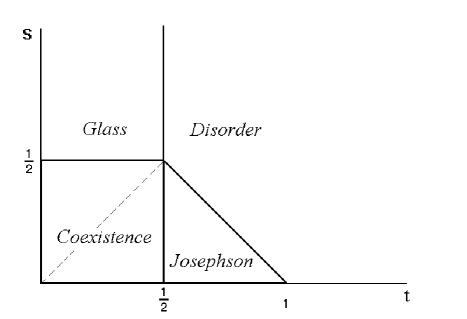
FIG. 2.: Phase diagram of a 2D junction in terms of s, the spread in random magnetic fields and $t$, which is proportional to temperature. The various phases, in terms of the Josephson order $z$ and the glass order $\Delta$ are: (i) Disordered phase with $z=\Delta=0$, (ii) Josephson phase with $z\neq 0,\;\Delta=0$, (iii) coexistence with both $z\neq 0,\;\Delta\neq 0$, and (iv) glass phase with $z=0,\;\Delta\neq 0$. The dashed line within the coexistence phase is where $\Delta$ changes sign.

The solutions for $z$ and $\Delta$ of Eqs. (62-65) determine the phase diagram. Consider first the Josephson ordered phase $z\neq 0,\Delta=0$. Expecting $\sigma_{0}<<1$ an expansion of Eq. (62) in powers of $\Delta/z$ yields $m\approx t\Delta/z$ so that $\sigma_{0}\approx e^{2}(z/\Delta_{c})^{2t}$ is indeed small. The solution for $z$ when $\Delta\rightarrow 0$ is equivalent to the replica symmetric case, Eq. (43) and is possible for $t<1-\sigma$.

Consider next an RSB solution $z=0,\Delta\neq 0$. Eq. (62) yields $m=2t$ and Eq. (64) leads to

$$\Delta/\Delta_{c}=(2tv_{0}/\Delta_{c})^{1/(1-2t)}$$ (66)

Thus a glass type phase is possible for $t<1/2$. (Curiously, a similar result is obtained for the $v$ term in 1st order RG, $\ell=2$ in Eq. (26), however, $G_{\alpha,\alpha}\sim 1/q^{4}$ at $q\rightarrow 0$, while here $G_{\alpha,\alpha}\sim 1/q^{2}$).

Finally consider a coexistence phase, where both $z$, $\Delta\neq 0$. It is remarkable that $m=2t$ is an exact solution even in this case, as can be checked by substitution in Eqs. (62,64,65). The resulting solutions are

$$\frac{z+\Delta}{\Delta_{c}} = \left(2t\frac{v_{0}}{\Delta_{c}}\right)^{1/(1-2t)}$$ (67)

$$\frac{z}{\Delta_{c}} = \mbox{e}^{-1}\left(\frac{u_{0}^{2}}{2tv_{0}\Delta_{c}}\right)^{1/(1-2s)}\,.$$ (68)

This coexistence phase is therefore possible at $t<1/2$ and $s<1/2$, as shown in the phase diagram, Fig. 2. It is interesting to note that $\Delta=0$ on some line within the coexistence phase, i.e. $\Delta$ changes sign continuously across this line. When $u_{0}\approx v_{0}$ this line is $s=t$, as shown by the dashed line in Fig. 2. This line is not a phase transition as far as the correlation $c(\bf{r})$ (Eq. (69) below) or the critical currents are concerned. We expect, however, that the slow relaxation phenomena, associated with the glass order, will disappear on this line.

The boundary $s=1/2$ of the coexistence phase is a continuous transition with $z\rightarrow 0$ at the boundary. On the other hand, the boundary at $t=1/2$ is a discontinuous transition, $z+\Delta\rightarrow 0$ from the left while $\Delta=0,\,z\neq 0$ on the right, i.e. both $\Delta$ and $z$ are discontinuous.

To identify the various phases we consider the correlation function

$$c(r)=\langle\cos\varphi_{\alpha}({\bf r})\cos\varphi_{\alpha}(0)\rangle=[\exp(-\phi_{+})+\exp(-\phi_{-})]/2$$ (69)

where

$$\phi_{\pm}=\int_{1/L}^{\sqrt{\Delta_{c}}}q\,dq[1\pm J_{0}(qr)]G_{\alpha,\alpha}(q)/2\pi\\$$ (70)

and the system size $L$ appears as a low momentum cutoff. Using $G_{\alpha,\alpha}(q)=\alpha(q)+\beta(q)+\gamma(q)$, the various correlations are summarized in Table I. The ordered phases have finite correlation lengths defined as $\lambda_{J}=z^{-1/2}$ for the Josephson length, $\lambda_{G}=\Delta^{-1/2}$ for the glass correlation length and $\lambda^{\prime}_{G}=(z+\Delta)^{-1/2}$ in the coexistence phase. It is curious to note that in the coexistence phase $G_{\alpha,\alpha}$ has a $(2t-1)/(q^{2}+z+\Delta)$ term. Since $z+\Delta\rightarrow 0$ much faster than $2t-1\rightarrow 0$ at the boundary $t=1/2$, this leads to an apparent divergence of $\lambda_{G}^{\prime}$; however, $\phi_{\pm}$ is finite at $t\rightarrow 1/2$ and the transition is of first order.

$\displaystyle\begin{array}[]{c|c|c|c}\mbox{phase}&G_{\alpha,\alpha}(q)&c(L)\;;\;\;L<\lambda_{J},\lambda_{G}&c(L)\;;\;\;L>\min(\lambda_{J},\lambda_{G})\\ \hline\cr\hline\cr\mbox{Disorder}&\frac{8\pi(t+s)}{q^{2}}&\left(\frac{L}{\lambda}\right)^{-4(t+s)}&\\ \hline\cr\mbox{Josephson}&\frac{8\pi(t+s)}{q^{2}+z}-\frac{8\pi sz}{(q^{2}+z)^{2}}&\left(\frac{L}{\lambda}\right)^{-4(t+s)}&\left(\frac{\lambda_{J}}{\lambda}\right)^{-4(t+s)}\\ \hline\cr\mbox{Glass}&\frac{4\pi(1+2s)}{q^{2}}+\frac{4\pi(2t-1)}{q^{2}+\Delta}&\left(\frac{L}{\lambda}\right)^{-4(t+s)}&\left(\frac{L}{\lambda}\right)^{-2(1+2s)}\left(\frac{\lambda_{G}}{\lambda}\right)^{-2(2t-1)}\\ \hline\cr\mbox{Coexistence}&\begin{array}[t]{l}\frac{4\pi(2t-1)}{q^{2}+z+\Delta}+\frac{4\pi(1+2s)}{q^{2}+z}\\ -\frac{4\pi z}{(q^{2}+z)^{2}}\end{array}&\left(\frac{L}{\lambda}\right)^{-4(t+s)}&\left(\frac{\min(L,\lambda_{G}^{\prime})}{\lambda}\right)^{-2(2t-1)}\left(\frac{\min(L,\lambda_{J})}{\lambda}\right)^{-2(1+2s)}\\ \hline\cr\end{array}$

TABLE I.: Correlations in junctions of size L; $c(L)$ determines $I_{c}$ via Eqs. (72, 73).

The phases with $z=0$ have power law correlations; for $L\rightarrow\infty$, $c(r)\sim r^{-4t-4s}$ in the disordered phase while $c(r)\sim r^{-2-4s}$ in the glass phase. The glass phase leads to stronger decrease of $c(r)$ then what would have been $c(r)$ in a disordered phase at $t<1/2$; a prefactor $(\lambda_{J}/\lambda)^{2(1-2t)}$ somewhat compensates for this reduction.

The phases with $z\neq 0$ have long range order. Note in particular the $z/(q^{2}+z)^{2}$ terms in $G_{\alpha,\alpha}$; these terms do not arise in RG since they are of higher order in $z$ and are of interest away from the transition line. Note that in the Josephson phase $v_{0}\approx u_{0}$ is assumed, so that $\sigma_{0}v_{0}\ll z$; otherwise the coefficient of $(q^{2}+z)^{-2}$ is modified.

The correlation $c(L)$ measures the fluctuation effect on $\langle\cos\varphi_{J}\rangle$ in a finite junction, i.e. $\langle\cos\varphi_{J}\rangle\approx\sqrt{c(L)}$, which is therefore related to the Josephson critical current $I_{c}$. The results for $c(L)$ are summarized in table I. Consider first a junction with $L<\lambda_{J}$ (which is always the case in the $z$=0 phases). The current flows through the whole junction and the system is equivalent to a point junction with an effective Gibbs free energy,

$$G_{J}^{eff}=E_{J}(L/\lambda)^{2}\sqrt{c(L)}\,\cos\varphi_{J}-(\phi_{0}/2\pi c)I^{ex}\varphi_{J}.$$ (71)

Here we assume (as at the end of section II) that point junction fluctuations can be ignored, i.e. $\phi_{0}I_{c}/2c>T$ and the critical current of Eq. (71) can be deduced by its mean field equation (see section V for actual data). Thus, the mean field value $I_{c1}^{0}$ (Eq. (10)) is reduced by the fluctuation factor, leading to a critical current

$$I_{c}=I_{c1}^{0}\sqrt{c(L)}\mbox{\hskip 85.35826pt}L<\lambda_{J}.$$ (72)

For $L<\lambda_{J},\lambda_{G}$ the parameters $\Delta$ and $z$ are no longer related to $\lambda_{J}$ or to $\lambda_{G}$; instead they are L dependent (Eq. (53) should be reevaluated leading to power laws of $L$). In particular $z$ affects $c(L)$ via the $(q^{2}+z)^{-2}$ terms by either a factor $\exp[2sz(L)L^{2}]$ (in the Josephson phase) or $\exp[z(L)L^{2}]$ (in the coexistence phase). Although of unusual form, these factors are neglected in table I since $zL^{2}<1$. The dominant dependence in a small area junction, $L<\lambda_{J},\lambda_{G}$ (for all phases) is a power law decrease of $c(L)$, leading to $I_{c}\sim L^{2-2t-2s}$.

For systems with $L>\lambda_{J}$, the current flows in an area $~{}L\lambda_{J}$ near the edges of the junction. The mean field value $I_{c2}^{0}$ (Eq. (10)) is reduced now by a factor $\lambda_{J}^{0}/\lambda_{J}$. Using $\langle\cos\varphi_{J}\rangle=\sqrt{c(L)}$ and $z=u_{0}\langle\cos\varphi_{J}\rangle=1/\lambda_{J}^{2}$ we obtain $\lambda_{J}=\lambda_{J}^{0}c^{-1/4}(L)$ with $\lambda_{J}^{0}=\lambda(\tau/8\pi E_{J})^{1/2}$, as in section II. The critical current is then

$$I_{c}=I_{c2}^{0}\sqrt[4]{c(L)}\mbox{\hskip 85.35826pt}L>\lambda_{J}$$ (73)

The relevant range of temperatures $T\ll\tau$ (see section II), for typical junction parameters, is most of the range $T<T_{c}$, excluding only $T$ very close to $T_{c}$. Thus $t\ll 1$ and our main interest is the coexistence to glass transition at $s=\frac{1}{2}$. This transition can be induced by a temperature change since $s=s(T)$ (see section III). Thus we consider $t\ll s$ for which $z\ll\Delta$ and $\lambda_{J}\gg\lambda_{G}\approx\lambda_{G}^{\prime}$. When the transition at $s=\frac{1}{2}$ is approached $\lambda_{J}$ diverges and for a given $L$ the system crosses into the regime $\lambda_{G}<L<\lambda_{J}$ (which includes the glass phase) where $c(L)\sim(L/\lambda)^{-4s}(\lambda_{G}/L)^{2}$ and $I_{c}\sim(L/\lambda)^{1-2s}$. Since $L\gg\lambda$ we predict a sharp decrease of $I_{c}$ at some temperature $T_{J}$ for which $s(T_{J})=\frac{1}{2}$; this is the finite size equivalent of the $L\rightarrow\infty$ phase transition.

V Discussion

We have derived the effective free energy for a 2D josephson junction (Appendix A) and studied it in presence of random magnetic fields. We show that a coupling between replicas of the form $\cos(\varphi_{\alpha}-\varphi_{\beta})$ is essential for describing the system. This coupling is generated by RG from the Josephson term in presence of the random fields, or also from disorder in the Josephson coupling, a disorder whose finite mean is $E_{J}$.

We find the phase diagram, Fig. 2, with four distinct phases defined in terms of a Josephson ordering $z\sim\langle\cos\varphi_{J}\rangle$ and a glass order parameter $\Delta$. At high temperatures thermal fluctuations dominate and the system is disordered, $z=\Delta=0$. Lowering temperature at weak disorder ($s<\frac{1}{2}$) allows formation of a Josephson phase, $z\neq 0,\,\Delta=0$. Further decrease of temperature leads by a first order transition to a coexistence phase where both $z,\Delta\neq 0$. The Josephson and coexistence phases have similar diagonal correlations (see table I). The main distinction between these phases is then the slow relaxation times typical of glasses. Finally, at strong disorder and low temperatures the glass phase with $z=0,\;\Delta\neq 0$ corresponds to destruction of the Josephson long range order by the quenched disorder.

Our main result, relevant to experimental data with $t\ll 1$, is the coexistence to glass transition at $s=\frac{1}{2}$. The critical behavior of $I_{c}(s)$ near this transition depends on the ratio $L/\lambda_{J}$; not too close to $s=\frac{1}{2}$ where $L>\lambda_{J}$ we have from Eq. (68, 73) $\ln I_{c}\sim 1/(1-2s)$ while closer to $s=\frac{1}{2}$ the divergence of $\lambda_{J}$ implies $L<\lambda_{J}$ with $I_{c}\sim(L/\lambda)^{1-2s}$. The junction ordering temperature $T_{J}$ corresponds to $s(T_{J})=\frac{1}{2}$ so that either $\ln I_{c}\sim-(T_{J}-T)^{-1}$ (not too close to $T_{J}$) or $\ln I_{c}\sim(T_{J}-T)\ln L/\lambda$ close to $T_{J}$.

We reconsider now the experimental data [1, 2, 3, 4, 5] where the junctions order at temperatures well below the $T_{c}$ of the bulk. In our scheme, this can correspond to a transition between the glass phase and the coexistence phase, a transition which may occur even at low temperatures $t\ll 1$ provided $s$ decreases with temperature. As discussed in section III, $s$ depends on a power of $\lambda$, in particular $s\sim\lambda^{2}$ for short junctions, the experimentally relevant case. Thus $s$ decreases with temperature since $\lambda$ is temperature dependent. We propose then that junctions with random magnetic fields (arising, e.g. from quenched flux loops in the bulk) may order at temperatures well below $T_{c}$ of the bulk.

From critical currents [1, 2] at $4.2K$ $I_{c}\approx 150-400\mu A$ we infer $E_{J}\approx 1-4K$ and $\lambda_{J}^{0}\approx 2-4\mu m$, the latter is somewhat below the junction sizes $L\approx 5-50\mu m$. For the more recent data on YBCO junctions [3, 4, 5] with $I_{c}\approx 0.4-6mA$ we obtain $\lambda_{J}^{0}\ll L$ and Eq. (73) applies. In fact, magnetic field dependence [4] and $I_{c}\sim L$ dependence [7] show directly that $\lambda_{J}<L$ is feasible.

We note also that mean field treatment of the effective free energy Eq. (71) is valid since thermal fluctuations of the effective point junction are weak (as assumed in sections II and IV), i.e. $\phi_{0}I_{c}/2c>T$. E.g., at $80K$ $\phi_{0}I_{c}/2c=T$ corresponds to $I_{c}\approx 1\mu A$ while the mean field $I_{c}$ at the temperatures where $I_{c}$ disappears, i.e. at $0.4-0.8T_{c}$, should be comparable to its low temperature values [1, 2, 3, 4, 5] of $I_{c}=0.1-6mA$. Thus $\phi_{0}I_{c}/2c\gg T$ and point junction type fluctuations can be neglected.

Other interpretations of the data assume that the composition of the barrier material is affected by the superconducting material and becomes a metal [3] N or even a superconductor [5] S’. In an SNS junction the coherence length in the metal is temperature dependent and affects $I_{c}$ while the onset of an SS’S junction obviously affects $I_{c}$. Note, however, that the SNS interpretation with $\ln I_{c}\sim-T^{1/2}$ is consistent with the $T$ dependence but leads to an inconsistent value of the coherence length [3]. In our scheme, $\ln I_{c}\sim(T_{J}-T)\ln L/\lambda$ is consistent with the data [3] of the $100\times 100\mu m^{2}$ junction showing a cusp in $I_{c}(T)$ near $T_{J}\approx 25K$. Further experimental data, and in particular the $L$ dependence of $I_{c}$, can determine the appropriate interpretation of the data.

The increasing research on large area junctions is motivated by device applications. The design of these junctions should consider the various types of disorder as studied in the present work. Furthermore, we believe that disordered large area junctions deserve to be studied since they exhibit novel glass phenomena. In particular the coexistence phase with both long range order and glass order is an unusual type of glass.

Acknowledgments: We thank S. E. Korshunov for valuable and stimulating discussions. This research was supported by a grant from the Israel Science Foundation.

A Free energy of a 2D Josephson junction

In this appendix we derive the effective free energy of a large area Josephson junction. In Appendix A.1 boundary conditions and the Josephson phase are defined. In Appendix A.2 the Gibbs free energy in presence of an external current is derived. In Appendices A.3, A.4 the Gibbs free energy is derived explicitly for superconductors in the Meissner state, i.e. no flux lines in the bulk; Appendix A.3 considers long junctions, i.e. $W>>\lambda$ (see Fig. 1) while Appendix A.4 considers short ones, $W<<\lambda$. Finally, in Appendix A.5 the free energy in presence of (quenched) flux loops in the bulk is derived.

1 Boundary conditions

The barrier between the superconductors (region I in Fig. 1) is defined by allowing currents $j_{z}(x,y)$ in the $z$ direction so that Maxwell’s relation for the vector potential ${\bf A}(x,y,z)$ is

$${\bf\nabla}\times{\bf\nabla}\times{\bf A}=(4\pi/c)j_{z}\hat{z}$$ (A1)

where $\hat{z}$ is a unit vector in the $z$ direction. There is no additional relation between $j_{z}$ and ${\bf A}$ (e.g. as in superconductors). This allows $j_{z}$ to be a fluctuating variable in thermodynamic averages.

Eq. (A1) implies that the magnetic field in the barrier ${\bf H}(x,y)={\bf\nabla}\times{\bf A}$ is $z$ independent and $H_{z}=0$; thus the currents $j_{x}$, $j_{y}=0$ as required.

Considering the superconductors in Fig. 1 we denote all 2D fields (i.e. $x$, $y$ components) at the right and left junction surfaces (i.e. $z=\pm d/2)$ with indices 1, 2, respectively. Boundary conditions are derived [18] by integrating ${\bf\nabla}\times{\bf A}$ around the dashed rectangle in Fig. 1, which since $j_{y}=0$, yields continuity of the parallel magnetic fields

$${\bf H}_{1}(x,y)={\bf H}_{2}(x,y)\,.$$ (A2)

Integrating ${\bf A}$ along the same rectangle yields for the vector potentials on the junction surfaces,

$$A_{1x}-A_{2x}+\int_{-d/2}^{d/2}(\partial A_{z}/\partial x)\,dz=dH_{y}$$ (A3)

and a similar relation interchanging $x$ and $y$. Introducing the phases $\varphi_{i}({\bf r})$, $i=1,2$ for the two superconductors and a gauge invariant vector potential

$${\bf A}_{i}^{\prime}({\bf r})={\bf A}_{i}({\bf r})-(\phi_{0}/2\pi){\bf\nabla}\varphi_{i}({\bf r})$$ (A4)

yields for ${\bf A}_{i}^{\prime}(x,y)$ on the junction surfaces

$${\bf A}_{1}^{\prime}(x,y)-{\bf A}_{2}^{\prime}(x,y)=d{\bf H}(x,y)\times\hat{z}-(\phi_{0}/2\pi){\bf\nabla}\varphi_{J}(x,y)$$ (A5)

where $\varphi_{J}(x,y)$ is the Josephson phase,

$$\varphi_{J}(x,y)\equiv\varphi_{1}(x,y)-\varphi_{2}(x,y)-(2\pi/\phi_{0})\int_{-d/2}^{d/2}A_{z}\,dz$$ (A6)

2 Gibbs free energy

In the presence of a given external current ${\bf j}^{ex}$ passing through the junction we separate the system into the sample with relevant fluctuations (e.g. superconductors with barrier) and an external environment in which ${\bf j}^{ex}$ is given. Thermodynamic quantities are then given by a Gibbs free energy ${\cal G}({\bf H})$ where ${\bf H}$ is the field outside the sample which determines ${\bf j}^{ex}$. The situation which is usually studied is such that ${\bf j}^{ex}$ does not flow through the sample [19] so that it is uniquely defined everywhere. We need to generalize this situation to the case in which ${\bf j}^{ex}$ flows through the sample, a generalization which to our knowledge has not been developed previously.

In standard electrodynamics [20], in addition to the space and time dependent electric and magnetic fields ${\bf E}$ and ${\bf H}$, respectively, one defines a free current ${\bf j}_{f}$, a displacement field ${\bf D}$ and an induction field ${\bf B}$ such that

$${\bf\nabla}\times{\bf H} = (4\pi/c){\bf j}_{f}+(1/c)\partial{\bf D}/\partial t$$ (A7)

$${\bf\nabla}\times{\bf E} = -(1/c)\partial{\bf B}/\partial t$$ (A8)

and only outside the sample ${\bf D}={\bf E}$, ${\bf B}={\bf H}$ and ${\bf j}_{f}={\bf j}^{ex}$. When the various electrodynamic fields change by a small amount, the change in the sample’s energy is the Poynting vector integrated over the sample surface S (with normal $d{\bf s}$) in time $dt$

$$-dt\frac{c}{4\pi}\int_{S}{\bf E}\times{\bf H}\,d{\bf s}=\int_{V}[\frac{1}{4\pi}{\bf H}\cdot d{\bf B}+\frac{1}{4\pi}{\bf E}\cdot d{\bf D}+{\bf E}\cdot{\bf j}_{f}\,dt]\,dV$$ (A9)

where integration is changed from the surface $S$ to the enclosed volume $V$ by Eq. (A8). When ${\bf j}^{ex}$ does not flow through the sample, ${\bf j}_{f}=0$ and neglect of ${\bf D}$ (for low frequency phenomena) leads to the usual energy change [19] $dE=\int{\bf H}\cdot d{\bf B}/4\pi$.

The general situation is described by keeping the surface integral in Eq. (A9) and in terms of the vector potential ${\bf A}$, where ${\bf E}=-(1/c)\partial{\bf A}\partial t$,

$$dE=\int_{S}\,d{\bf A}\times{\bf H}\,d{\bf s}/4\pi$$ (A10)

Thus the surface values of ${\bf A}$ and ${\bf H}$ (parallel to the surface) determine the energy exchange $dE$ and there is no need to specify an ${\bf H}$ or a ${\bf j}_{f}$ inside the sample, where in fact they are not uniquely determined.

Since ${\bf H}$ (on the surface) is determined by ${\bf j}^{ex}$ (via Eq. (A8) outside the sample) we define a Gibbs free energy ${\cal G}({\bf H})$ by a Legendre transform

$${\cal G}({\bf H})={\cal F}-(1/4\pi)\int_{S}{\bf A}\times{\bf H}\,d{\bf s}$$ (A11)

${\bf A}$ is determined now by a minimum condition $\delta{\cal G}/\delta{\bf A}=0$ which indeed reproduces Eq. (A10).

We apply now Eq. (A11) to the Josephson junction system. We assume a time independent current ${\bf j}^{ex}$, i.e. ${\bf\nabla}\times{\bf H}=(4\pi/c){\bf j}^{ex}$ outside the sample and that the same current ${\bf j}^{ex}$ flows through both superconductor-normal (SN) surfaces (e.g. the superconductors close into a loop or that the current source is symmetric). Consider now the surface $S_{1}$ of superconductor 1, which includes the superconductor-normal (SN) surface and the superconductor-vacuum (SV) surface. The boundary of $S_{1}$ is a loop $J$ which encircles the junction surface, oriented with normal ${+\hat{z}}$. In terms of the gauge invariant vector ${\bf A}^{\prime}={\bf A}-(\phi_{0}/2\pi){\bf\nabla}\varphi_{1}$, assuming ${\bf j}^{ex}$ is time independent, $\partial{\bf E}/\partial t=0$ and using

$\displaystyle{\bf\nabla}\varphi_{1}\times{\bf H}={\bf\nabla}\times(\varphi_{1}{\bf H})-(4\pi/c)\varphi_{1}\,{\bf j}^{ex}$

we obtain

$$\int_{S_{1}}{\bf A}\times{\bf H}\,d{\bf s}=\frac{\phi_{0}}{2\pi}[\oint_{J}\varphi_{1}{\bf H}\cdot\,d{\bf l}-(4\pi/c)\int\varphi_{1}{\bf j}^{ex}\cdot d{\bf s}]+\int_{S_{1}}{\bf A}^{\prime}\times{\bf H}\cdot d{\bf s}$$ (A12)

The ${\bf j}^{ex}\cdot d{\bf s}$ term for both superconductors involves the difference $\varphi_{1}-\varphi_{2}$ of the phases on the two SN surfaces. This difference [17] is related to the chemical potential difference in the external circuit so that the corresponding term is $\varphi_{J}$ independent.

Consider next the insulator-vacuum (IV) surface. Since $H_{z}=0$ in the insulator only the $A_{z}H_{y}$ or $A_{z}H_{x}$ terms contribute with

$$\int_{IV}{\bf A}\times{\bf H}\,d{\bf s}=-\oint_{J}{\bf H}\cdot\,d{\bf l}\int_{-d/2}^{d/2}A_{z}\,dz$$ (A13)

Combining Eq. (A12), the similar term for superconductor 2 and Eq. (A13), (ignoring $\varphi_{J}$ independent terms) we obtain,

$${\cal G}({\bf H})={\cal F}-\frac{1}{4\pi}\int_{SV+SN}{\bf A}^{\prime}\times{\bf H}\cdot d{\bf s}-\frac{\phi_{0}}{8\pi^{2}}\oint\varphi_{J}{\bf H}\cdot\,d{\bf l}.$$ (A14)

3 Long superconductors

We derive here an explicit free energy, in terms of the Josephson phase, for the case $W>>\lambda_{1},\lambda_{2}$ (see Fig. 1), where $\lambda_{i}$ (i=1,2) are the London penetration lengths of the two superconductors, respectively. The incoming current ${\bf j}^{ex}(x,y)$ is parallel to the $\hat{z}$ axis.

Consider the free energy [19] of superconductor 1 (suppressing the subscript 1 for now)

$${\cal F}=\frac{1}{8\pi}\int_{z\geq d/2}d^{3}r[\frac{1}{\lambda^{2}}(\frac{\phi_{0}}{2\pi}{\bf\nabla}\varphi-{\bf A})^{2}+({\bf\nabla}\times{\bf A})^{2}]$$ (A15)

The superconductor is assumed to have no flux lines, i.e. $\varphi({\bf r})$ is nonsingular. The vector ${\bf A}^{\prime\prime}={\bf A}-(\phi_{0}/2\pi){\bf\nabla}\varphi$ has then 3 independent components (no gauge condition on ${\bf A}^{\prime\prime}$) and ${\bf\nabla}\times{\bf A}^{\prime\prime}={\bf\nabla}\times{\bf A}$. The partition function involves integration on all vectors ${\bf A}^{\prime\prime}$ and on its boundary values ${\bf A}^{\prime}_{s}({\bf r}_{s})$ on the boundary ${\bf r}_{s}$ of the superconductor,

$$Z=\int{\cal D}{\bf A}^{\prime}_{s}({\bf r}_{s})\int{\cal D}{\bf A}^{\prime\prime}({\bf r})\exp[-{\cal F}\{{\bf A}^{\prime\prime}({\bf r}),{\bf A}^{\prime}_{s}({\bf r}_{s}\}/T]\,.$$ (A16)

We shift now the integration field from ${\bf A}^{\prime\prime}$ to $\delta{\bf A}^{\prime}$ where ${\bf A}^{\prime\prime}={\bf A}^{\prime}+\delta{\bf A}^{\prime}$ and ${\bf A}^{\prime}$ is the solution of $\delta F/\delta{\bf A}^{\prime}=0$, i.e.

$${\bf\nabla}\times{\bf\nabla}\times{\bf A}^{\prime}=-{\bf A}^{\prime}/\lambda^{2}$$ (A17)

with ${\bf A}^{\prime}={\bf A}^{\prime}_{s}$ at the boundaries; thus $\delta{\bf A}^{\prime}({\bf r}_{s})=0$. Since F is Gaussian, $F({\bf A}^{\prime}+\delta{\bf A}^{\prime})=F({\bf A}^{\prime})+F(\delta{\bf A}^{\prime})$ and the integration on $\delta{\bf A}^{\prime}$ is a constant independent of ${\bf A}^{\prime}_{s}({\bf r}_{s})$. Thus

$\displaystyle Z\sim\int{\cal D}{\bf A}^{\prime}_{s}({\bf r}_{s})\exp[-{\cal F}\{{\bf A}^{\prime}({\bf r})\}/T]$

where

$${\cal F}\{{\bf A}^{\prime}\}=\frac{1}{8\pi}\int d^{3}r[\frac{1}{\lambda^{2}}{\bf A}^{\prime 2}+{\bf\nabla}\times{\bf A}^{\prime})^{2}]$$ (A18)

Note that Eq. (A17) implies ${\bf\nabla}\cdot{\bf A}^{\prime}=0$ and therefore ${\bf\nabla}^{2}{\bf A}^{\prime}={\bf A}^{\prime}/\lambda^{2}$. Note also that the currents obey ${\bf j}=-(c/4\pi\lambda^{2}){\bf A}^{\prime}$.

We are interested in boundary fields at the barrier which are 2D vectors, e.g.

$\displaystyle{\bf A}^{\prime}_{1}(x,y)\equiv(A_{1x}^{\prime}(x,y),A_{1y}^{\prime}(x,y))\;.$

The effect of these fields decays on a scale $\lambda$ so that for $z>>\lambda$, ${\bf A}^{\prime}\sim{\hat{z}}j^{ex}(x,y)$ also obeys London’s equation $\lambda^{2}\nabla^{2}j^{ex}=j^{ex}$. Therefore $j^{ex}$ is confined to a layer of thickness $\lambda$ near the SV surface. The solution for $z\geq d/2$ has the form

$$[A_{x}^{\prime}({\bf r}),A_{y}^{\prime}({\bf r})]={\bf A}_{1}^{\prime}(x,y)\exp[-(z-d/2)/\lambda]$$ (A19)

$$A_{z}^{\prime}({\bf r})=\lambda{\bf\nabla}{\bf A}_{1}^{\prime}(x,y)\exp[-(z-d/2)/\lambda]-(4\pi\lambda^{2}/c)j^{ex}(x,y)$$ (A20)

This ansatz is a solution of London’s equation (A17) provided that ${\bf A}_{1}^{\prime}(x,y)$ is slowly varying on the scale of $\lambda$. The corresponding magnetic fields are

$$({\bf\nabla}\times{\bf A})_{x}^{\prime} = (1/\lambda)A_{y}^{\prime}-(4\pi\lambda^{2}/c)\partial_{y}j^{ex}+O(\nabla^{2}{\bf A}_{1}^{\prime})$$ (A21)

$$({\bf\nabla}\times{\bf A})_{y}^{\prime} = -(1/\lambda)A_{x}^{\prime}-(4\pi\lambda^{2}/c)\partial_{x}j^{ex}+O(\nabla^{2}{\bf A}_{1}^{\prime})$$ (A22)

Since eventually ${\bf A}_{1}^{\prime}\sim{\bf\nabla}\varphi_{J}$ (Eq (A26) below) we evaluate ${\cal F}$ by neglecting terms with derivatives of ${\bf A}_{1}^{\prime}$. Some care is, however, needed in evaluating cross terms with $j^{ex}$, which is not slowly varying. Thus, $\int A_{z}^{\prime 2}({\bf r})$ from Eq. (A20) involves

$\displaystyle\int j^{ex}{\bf\nabla}\cdot{\bf A}_{1}^{\prime}\,dxdy=-\int{\bf A}_{1}^{\prime}\cdot{\bf\nabla}j^{ex}\,dxdy$

which cannot be neglected. Note that the line integral on the SV surface vanishes since on this surface the perpendicular component of ${\bf A}_{1}^{\prime}$ is zero, i.e. no currents flowing into vacuum. The $O(\nabla^{2}{\bf A}_{1}^{\prime})$ terms in (Eq. (A22) can be neglected since their product with $j^{ex}$ cannot be partially integrated without SV line integrals.

The cross terms from squaring Eqs. (A20,A22) involve

$\displaystyle\int[j^{ex}{\bf\nabla}\cdot{\bf A}_{1}^{\prime}+{\bf A}_{1}^{\prime}\cdot{\bf\nabla}j^{ex}]\,dxdy=\int{\bf\nabla}\cdot(j^{ex}{\bf A}_{1}^{\prime})\,dxdy=0\,.$

For superconductor 2 with $z<-d/2$ the solution has the form of Eq (A20) with ${\bf A}_{2}^{\prime}(x,y)$ replacing ${\bf A}_{1}^{\prime}(x,y)$, the $z$ dependence has $\exp[(z+d/2)/\lambda_{2}]$ and $-{\bf\nabla}\cdot{\bf A}^{\prime}_{2}$ replaces ${\bf\nabla}\cdot{\bf A}^{\prime}_{1}$ in the equation for $A_{z}^{\prime}$. For both superconductors (i=1,2), after $z$ integration, we obtain

$${\cal F}_{i}=\int dx\,dy\,{\bf A}_{i}^{\prime 2}(x,y)/8\pi\lambda_{i}+O(\partial{\bf A}_{i}^{\prime})^{2}.$$ (A23)

.

Next we use the boundary conditions Eqs. (A2, A5) to relate ${\bf A}_{i}^{\prime}$ to $\varphi_{J}$. Equations (A2, A22) yield

$${\bf A}_{1}^{\prime}/\lambda_{1}-(4\pi\lambda_{1}^{2}/c){\bf\nabla}j_{1}^{ex}=-{\bf A}_{2}^{\prime}/\lambda_{2}-(4\pi\lambda_{2}^{2}/c){\bf\nabla}j_{2}^{ex}+O(\partial{\bf A}_{i}^{\prime})^{2}$$ (A24)

while Eq. (A5) yields

$${\bf A}_{1}^{\prime}-{\bf A}_{2}^{\prime}=d[-{\bf A}_{1}^{\prime}/\lambda_{1}+(4\pi\lambda_{1}^{2}/c){\bf\nabla}j_{1}^{ex}]-(\phi_{0}/2\pi){\bf\nabla}\varphi_{J}$$ (A25)

Since ${\bf\nabla}j^{ex}$ is not slowly varying, the ansatz Eq. (A20) is consistent (i.e. ${\bf A}^{\prime}_{i}$ are slowly varying) only if the junction is symmetric, $j_{1}^{ex}(x,y)=j_{2}^{ex}(x,y)$, $\lambda\equiv\lambda_{1}=\lambda_{2}$ and that the limit $d/\lambda\rightarrow 0$ is taken. Thus,

$${\bf A}_{1}^{\prime}=-{\bf A}_{2}^{\prime}=-(\phi_{0}/4\pi)^{2}{\bf\nabla}\varphi_{J}$$ (A26)

The magnetic energy in the barrier is neglected since it involves $d/\lambda$. The total free energy, from Eqs. (A23,A26) is then

$${\cal F}={\cal F}_{1}+{\cal F}_{2}=\frac{1}{4\pi\lambda}\left(\frac{\phi_{0}}{4\pi}\right)^{2}\int dxdy({\bf\nabla}\varphi_{J})^{2}$$ (A27)

If $j^{ex}=0$, Eqs. (A23,A26) are valid also for nonsymmetric junctions and ${\cal F}$ has the form  (A27) with $2\lambda$ replaced by $\lambda_{1}+\lambda_{2}+d$.

We proceed to find the Gibbs terms in (A14). Since Eq. (A22) and the constraint of no current flowing into the vacuum, ${\bf A}^{\prime}\times{\hat{z}}\cdot d{\bf l}=0$ yield ${\bf H}_{SV}=-(4\pi\lambda^{2}/c){\bf\nabla}j^{ex}\times{\hat{z}}$ on the SV surface, the loop integral becomes

$$\oint_{J}\varphi_{J}{\bf H}\cdot d{\bf l}=(4\pi\lambda^{2}/c)\oint_{J}\varphi_{J}{\bf\nabla}j^{ex}\cdot d{\bf l}\times{\hat{z}}$$ (A28)

For the SV surface integration we use again ${\bf H}_{SV}$ so that for superconductor 1,

$$\int_{SV_{1}}{\bf A}^{\prime}\times{\bf H}\cdot d{\bf s}=-(4\pi\lambda^{4}/c)\int_{SV_{1}}A_{z}^{\prime}{\bf\nabla}j^{ex}\cdot d{\bf s}$$

$$=(4\pi\lambda^{2}/c)\int{\bf A}_{1}^{\prime}\cdot{\bf\nabla}j^{ex}\,dxdy+O(\nabla^{2}{\bf A}_{1}^{\prime},\varphi_{J}\mbox{ independent terms})$$

where ${\bf\nabla}j^{ex}\cdot d{\bf s}$ is replaced by $\nabla^{2}j^{ex}\,dxdydz$ as $j^{ex}$ has dominant $x,y$ dependence. Using Eq. (A26) and adding terms for both superconductors leads to

$\displaystyle\int_{SV}{\bf A}^{\prime}\times{\bf H}\cdot d{\bf s}=\frac{2\phi_{0}}{c}\int\varphi_{J}\,j^{ex}\,dxdy-\frac{\phi_{0}}{2\pi}\oint_{J}\varphi_{J}{\bf H}\cdot d{\bf l}$

Finally we obtain,

$${\cal G}=\int dxdy\left[\frac{1}{4\pi\lambda}\left(\frac{\phi_{0}}{4\pi}\right)^{2}({\bf\nabla}\varphi_{J})^{2}-\frac{\phi_{0}}{2\pi c}\varphi_{J}\,j^{ex}\right]$$ (A29)

Adding the Josephson tunneling term $\sim\cos\varphi_{J}$ leads to Eqs. (1,3).

4 Short superconductors

Consider superconductors with length $W_{1},W_{2}<<\lambda_{1},\lambda_{2}$ (see Fig. 1). The $\exp(-z/\lambda_{1})$ in Eq. (A20) can be expanded to terms linear in $z$. Since now both $\exp(\pm z/\lambda_{1})$ are allowed at $z>0$, there are two slowly varying surface fields ${\bf A}_{1}$, ${\bf H}_{1}$,

$$[A_{x}^{\prime},A_{y}^{\prime}] = {\bf A}_{1}^{\prime}(x,y)+z{\bf H}_{1}(x,y)\times{\hat{z}}+O(z^{2})$$ (A30)

$$A_{z}^{\prime} = A_{1z}^{\prime}-z{\bf\nabla}\cdot{\bf A}_{1}^{\prime}+O(z^{2})$$ (A31)

and the magnetic field is

$${\bf H}={\bf H}_{1}(x,y)-(z/\lambda_{1}^{2}){\bf A}_{1}^{\prime}(x,y)\times{\hat{z}}+O(z^{2},\partial A_{z}^{\prime})$$ (A32)

The $x,y$ components of ${\bf H}={\bf H}_{1}^{ex}$ at $z=W_{1}$ define the boundary conditions,

$$H_{1x}-(W_{1}/\lambda_{1}^{2})A_{1y}^{\prime} = H_{1x}^{ex}$$ (A33)

$$H_{1y}+(W_{1}/\lambda_{1}^{2})A_{1x}^{\prime} = H_{1y}^{ex}$$ (A34)

and similarly ${\bf H}_{2}^{ex}$ at $z=-W_{2}$.

$$H_{2x}+(W_{2}/\lambda_{2}^{2})A_{2y}^{\prime} = H_{2x}^{ex}$$ (A35)

$$H_{2y}-(W_{2}/\lambda_{2}^{2})A_{2x}^{\prime} = H_{2y}^{ex}$$ (A36)

Equations (A34,A36) and the boundary conditions (A2,A5) at the junction determine all the fields ${\bf A}^{\prime}_{i},{\bf H}_{i}$ in terms of ${\bf H}_{i}^{ex}$ and $\varphi_{J}$, e.g.

$$A_{1x}^{\prime} = \frac{\lambda_{1}^{2}}{\lambda_{1}^{2}W_{2}+\lambda_{2}^{2}W_{1}+dW_{1}W_{2}}[(\lambda_{2}^{2}+W_{2}d)H_{1y}^{ex}-\lambda_{2}^{2}H_{2y}^{ex}-W_{2}(\phi_{0}/2\pi)\partial_{x}\varphi_{J}]$$ (A37)

$$A_{2x}^{\prime} = \frac{-\lambda_{2}^{2}}{\lambda_{1}^{2}W_{2}+\lambda_{2}^{2}W_{1}+dW_{1}W_{2}}[(\lambda_{1}^{2}+W_{1}d)H_{2y}^{ex}-\lambda_{1}^{2}H_{1y}^{ex}-W_{1}(\phi_{0}/2\pi)\partial_{x}\varphi_{J}]$$ (A38)

$$H_{1y} = \frac{\lambda_{2}^{2}W_{1}H_{2y}^{ex}+\lambda_{1}^{2}W_{2}H_{1y}^{ex}+W_{1}W_{2}(\phi_{0}/2\pi)\partial_{x}\varphi_{J}}{\lambda_{1}^{2}W_{2}+\lambda_{2}^{2}W_{1}+dW_{1}W_{2}}$$ (A40)

The boundary fields ${\bf H}_{i}^{ex}$ need to be slowly varying (of order ${\bf\nabla}\varphi_{J})$ so that Eq. (A40) is slowly varying; thus $H_{z}$, $A_{iz}\sim\nabla^{2}\varphi_{J}$ can be neglected.

The free energy (A18), to leading order in $W_{i}/\lambda_{i}$ is

$${\cal F}_{1}=(W_{1}/8\pi\lambda_{1}^{2})\int{\bf A}_{1}^{\prime 2}(x,y)\,dxdy+O((W_{1}/\lambda_{1})^{3}({\bf\nabla}\varphi_{J})^{2},(W_{1}/\lambda_{1})^{2}{\bf\nabla}\varphi_{J}\cdot{\bf H}_{1}^{ex})$$ (A41)

Ignoring $\varphi_{J}$ independent terms,

$${\cal F}_{1}+{\cal F}_{2}= \frac{\phi_{0}}{16\pi^{2}}\int dx\,dy\left\{\frac{\phi_{0}}{2\pi}\frac{W_{1}(W_{2}\lambda_{1})^{2}+W_{2}(W_{1}\lambda_{2})^{2}}{(\lambda_{1}^{2}W_{2}+\lambda_{2}^{2}W_{1}+dW_{1}W_{2})^{2}}({\bf\nabla}\varphi_{J})^{2}\right.$$ (A42)

$$\left.-2d\frac{\lambda_{1}^{2}W_{2}H_{1y}^{ex}+\lambda_{2}^{2}W_{1}H_{2y}^{ex}}{(\lambda_{1}^{2}W_{2}+\lambda_{2}^{2}W_{1}+dW_{1}W_{2})^{2}}\partial_{x}\varphi_{J}+(x\leftrightarrow y)\right\}$$ (A44)

The free energy in the barrier

$${\cal F}_{I}=(d/8\pi)\int dxdy{\bf H}_{1}^{2}(x,y)$$ (A45)

precisely cancels the terms linear in ${\bf\nabla}\varphi_{J}$ in (A44) so that

$${\cal F}=\frac{1}{8\pi}\left(\frac{\phi_{0}}{2\pi}\right)^{2}\frac{W_{1}W_{2}}{\lambda_{1}^{2}W_{2}+\lambda_{2}^{2}W_{1}}\int dxdy({\bf\nabla}\varphi_{J})^{2}.$$ (A46)

Considering next the Gibbs term, the SV surface involves $A_{z}^{\prime}$ or $H_{z}$ which are neglected. The SN surface involves ${\bf A}^{\prime}(z=W_{1})={\bf A}_{1}+O(W_{1}^{2}\partial\varphi_{J})$, hence

$$-\frac{1}{4\pi}\int_{SN}{\bf A}^{\prime}\times{\bf H}\cdot d{\bf s} = \frac{\phi_{0}}{8\pi^{2}}\int dxdy\frac{\lambda_{1}^{2}W_{2}H_{1y}^{ex}+\lambda_{2}^{2}W_{1}H_{2y}^{ex}}{\lambda_{1}^{2}W_{2}+\lambda_{2}^{2}W_{1}}\partial_{x}\varphi_{J}-(x\leftrightarrow y)+...$$ (A47)

$$= -\frac{\phi_{0}}{2\pi c}\int dx\,dy\,j^{ex}\varphi_{J}+\frac{\phi_{0}}{8\pi^{2}}\oint_{J}\varphi_{J}{\bf H}\cdot d{\bf l}+...$$ (A48)

where higher order terms in $W_{i}/\lambda_{i}$ and $\varphi_{J}$ independent terms are ignored, and the fact that ${\bf H}\cdot{\bf l}$ is $z$ independent on the SV surface is used (this arises from zero current into the vacuum and neglecting $H_{z}$). The current $j^{ex}$ is defined here as an average of the currents on both sides, $j_{i}^{ex}=({\bf\nabla}\times{\bf H}_{i}^{ex})_{z}$ (which locally may differ), i.e.

$$j^{ex}=\frac{\lambda_{1}^{2}W_{2}j_{1}^{ex}+\lambda_{2}^{2}W_{1}j_{2}^{ex}}{\lambda_{1}^{2}W_{2}+\lambda_{2}^{2}W_{1}}$$ (A49)

The Gibbs free energy is finally,

$${\cal G}={\cal F}-(\phi_{0}/2\pi c)\int dxdyj^{ex}(x,y)\varphi_{J}(x,y)$$ (A50)

with ${\cal F}$ given by Eq. (A46).

5 Junctions with bulk flux loops

Consider a junction with flux loops in the bulk of the superconductors. These loops induce magnetic fields which couple to $\varphi_{J}$. To derive this coupling we decompose the superconducting phase into singular $\varphi_{s}$ and nonsingular $\varphi_{ns}$ parts, i.e.

$\displaystyle{\bf\nabla}\times{\bf\nabla}(\varphi_{s}+\varphi_{ns})={\bf\nabla}\times{\bf\nabla}\varphi_{s}\neq 0\,.$

Define a 3 component vector ${\bf A}^{\prime\prime}={\bf A}-(\phi_{0}/2\pi){\bf\nabla}\varphi_{ns}$ so that the free energy Eq. (A15) is

$$F=\frac{1}{8\pi}\int d^{3}r[\frac{1}{\lambda^{2}}(\frac{\phi_{0}}{2\pi}{\bf\nabla}\varphi_{s}-{\bf A}^{\prime\prime})^{2}+({\bf\nabla}\times{\bf A}^{\prime\prime})^{2}]$$ (A51)

We shift the integration field ${\bf A}^{\prime\prime}$ by ${\bf A}^{\prime\prime}\rightarrow{\bf A}^{\prime\prime}+\delta{\bf A}^{\prime\prime}$ (as in section A.3) where $\delta{\bf A}^{\prime\prime}=0$ at the boundaries and ${\bf A}^{\prime\prime}$ satisfies $\delta F/\delta{\bf A}^{\prime\prime}=0$, i.e.

$${\bf\nabla}\times{\bf\nabla}\times{\bf A}^{\prime\prime}=[(\phi_{0}/2\pi){\bf\nabla}\varphi_{s}-{\bf A}^{\prime\prime}]/\lambda^{2}$$ (A52)

Since ${\cal F}$ is Gaussian in ${\bf A}^{\prime\prime}$, the integration on $\delta{\bf A}^{\prime\prime}$ decouples from that of $\varphi_{s}$ and the boundary values. Define now ${\bf A}^{\prime\prime}={\bf A}^{\prime}+{\bf A}_{s}$ where ${\bf A}_{s}$ is a specific solution of Eq. (A52) and ${\bf A}^{\prime}$ is the general solution of the homogeneous part of (A52), ${\bf\nabla}\times{\bf\nabla}\times{\bf A}^{\prime}=-{\bf A}^{\prime}/\lambda^{2}$, which depends on boundary conditions, i.e. on $\varphi_{J}$.

Substituting Eq. (A52) for ${\bf A}_{s}$ in Eq. (A51) yields

$${\cal F}=\frac{1}{8\pi}\int d^{3}r[\frac{1}{\lambda^{2}}(\lambda^{2}{\bf\nabla}\times{\bf\nabla}\times{\bf A}_{s}-{\bf A}^{\prime})^{2}+({\bf\nabla}\times{\bf A}^{\prime}+{\bf\nabla}\times{\bf A}_{s})^{2}].$$ (A53)

In the absence of flux loops ${\bf\nabla}\times{\bf A}_{s}=0$ and Eq. (A53) reduces to the previous ${\cal F}({\bf A}^{\prime})$ as in Eq. (A18). The terms which depend only on ${\bf A}_{s}$ represent energies of flux loops in the bulk and affect the thermodynamics of the bulk superconductors. Here we are interested in temperatures well below $T_{c}$ of the bulk so that fluctuations of these flux loops are very slow and are then sources of frozen magnetic fields. The thermodynamic average is done only on the boundary fields which determine ${\bf A}^{\prime}$, and are coupled to ${\bf A}_{s}$ by the cross terms in Eq. (A53),

$${\cal F}_{s} = (1/8\pi)\int d^{3}r[-2{\bf A}^{\prime}\cdot{\bf\nabla}\times{\bf\nabla}\times{\bf A}^{\prime}+2{\bf\nabla}\times{\bf A}^{\prime}\cdot{\bf\nabla}\times{\bf A}_{s}]$$ (A54)

$$= (1/4\pi)\int_{S}({\bf A}^{\prime}\times{\bf\nabla}\times{\bf A}_{s})\cdot d{\bf s}$$ (A55)

The surface values of ${\bf A}^{\prime}$ are determined by $\varphi_{J}$. The SV surface involves $z$ integration of ${\bf\nabla}\times{\bf A}_{s}$ with either $\exp(\pm z/\lambda)$, Eq. (A20), or a linear function, Eq. (A31). In either case the randomness in ${\bf\nabla}\times{\bf A}_{s}$ causes this integral to vanish. The relevant surface in Eq. (A55) is therefore the junction surface.

B Hierarchical Replica Symmetry Breaking

In this appendix we examine the full replica symmetry breaking formalism (RSB) and show that it reduces to the one step symmetry breaking solution, as studied in section IV. The method of RSB is based [15, 16] on a representation of hierarchical matrices $A_{ab}$ in replica space in terms of their diagonal $\tilde{a}$ and a one parameter function $a(u)$, i.e. $A_{ab}\rightarrow[\tilde{a},a(u)]$. In our case $A_{ab}$ is related to the inverse Green’s function $G^{-1}_{ab}$ which was obtained by Gaussian Variational Method (GVM).

To derive this representation, consider the hierarchical form of a matrix $\hat{A}$,

$$\hat{A}=\sum_{i=0}^{k}a_{i}(\hat{C}_{i}-\hat{C}_{i+1})+\tilde{a}\hat{I}$$ (B1)

Here $\hat{C}_{i}$ is $n\times n$ matrix whose nonzero elements are blocks of size $m_{i}\times m_{i}$ along the diagonal; each matrix element within the blocks is equal to one; the last matrix equals the unit matrix $\hat{C}_{k+1}=\hat{I}$. The matrices $\hat{C}_{i}$ satisfy relations which are useful for finding the representation of the product of matrices $\hat{A}\hat{B}$ . Since the hierarchy is for $m_{i}/m_{i+1}$ integers, we have

$$\hat{C}_{i} = \sum_{j=i}^{k}(\hat{C}_{j}-\hat{C}_{j+1})+\hat{I}$$ (B2)

$$\hat{C}_{i}\hat{C}_{j} = \left\{\begin{array}[]{ll}m_{i}\hat{C}_{j}\mbox{\hskip 85.35826pt $j\leq i$},\\ m_{j}\hat{C}_{i}\mbox{\hskip 85.35826pt $j>i$}\end{array}\right.$$ (B5)

The matrix product with a matrix $\hat{B}$,

$$\hat{B}=\sum_{i=0}^{k}b_{i}(\hat{C}_{i}-\hat{C}_{i+1})+\tilde{b}\hat{I}$$ (B6)

is found to be

$$\hat{A}\hat{B}=\sum_{j=0}^{k}(\hat{C}_{j}-\hat{C}_{j+1})[\sum_{i=j+1}^{k}(a_{i}b_{j}+a_{j}b_{i})\,dm_{i}-a_{j}b_{j}m_{j+1}+\sum_{i=0}^{j}a_{i}b_{i}\,dm_{i}]+\hat{I}[\sum_{i=0}^{k}a_{i}b_{i}\,dm_{i}+\tilde{a}\tilde{b}]\,.$$ (B7)

where $dm_{i}=m_{i}-m_{i+1}$.

In the limit $n\rightarrow 0$ $m_{i}$ becomes a continuum variable $u$ in the range $0<u<1$ and $a_{i}$ becomes a function $a(u)$; thus the matrix $\hat{A}$ is represented by $[\tilde{a},a(u)]$. The product of two matrices, using Eq.(B7), becomes $\hat{A}\hat{B}\rightarrow[\tilde{c},c(u)]$ where

$$\tilde{c} = \tilde{a}\tilde{b}-<ab>$$ (B8)

$$c(u) = (\tilde{a}-<a>)b(u)+(\tilde{b}-<b>)a(u)-\int_{0}^{u}[a(u)-a(v)][b(u)-b(v)]dv$$ (B9)

and $<a>=\int_{0}^{1}a(u)du$.

To find the inverse $\hat{B}=\hat{A}^{-1}$ we solve for $\tilde{c}=1$, $c(u)=0$ and find

$$\tilde{b}-b(u)=\frac{1}{u(\tilde{a}-<a>-[a](u))}-\int_{u}^{1}\frac{dv}{v^{2}(\tilde{a}-<a>-[a](v))}$$ (B10)

$$\tilde{b}=\frac{1}{\tilde{a}-<a>}[1-\int_{0}^{1}\frac{dv\,[a](v)}{v^{2}(\tilde{a}-<a>-[a](v))}-\frac{a(0)}{\tilde{a}-<a>}]$$ (B11)

$$[a](u)\equiv ua(u)-\int_{0}^{u}dv\,a(v)\,.$$ (B12)

The inverse Green’s function is from Eq. (40)

$$4\pi G_{ab}^{-1}(q)=\frac{1}{2t}[\delta_{ab}(z+q^{2})-v_{0}\sigma_{ab}-q^{2}s/t]$$ (B13)

which for $\hat{\sigma}\rightarrow[\tilde{\sigma},\sigma(u)]$ parameterizes as $[\tilde{a}_{q},a_{q}(u)]$ with

$$\tilde{a}_{q} = \frac{1}{2t}[q^{2}(1-s/t)+z-v_{0}\tilde{\sigma}]$$ (B14)

$$a_{q}(u) = -\frac{1}{2t}[q^{2}s/t+v_{0}\sigma(u)]$$ (B15)

Since the sum on each row of $\hat{\sigma}$ vanishes (Eq. (41) we obtain $\tilde{\sigma}=<\sigma>$. Therefore the denominator under the integration in Eqs. (B10,B11) assumes the form

$$\tilde{a}_{q}-<a_{q}>-[a_{q}](u)=\frac{1}{2t}(q^{2}+z+\Delta(u))$$ (B16)

where the order parameter $\Delta(u)$ is defined by $\Delta(u)=v_{0}[\sigma](u)$. From Eq. (B10) the representation of the Green’s function takes the form $(4\pi)G_{ab}\rightarrow[\tilde{b}_{q},b_{q}(u)]$ with

$$\tilde{b}_{q}-b_{q}(u)=2t[\frac{1}{u[q^{2}+z+\Delta(u)]}-\int_{u}^{1}\frac{dv}{v^{2}[q^{2}+z+\Delta(v)]}]\,.$$ (B17)

The GVM equation for $\sigma(u)$ is from Eq. (41) $\sigma(u)=\exp[-B(u)]$, where from Eq. (37)

$$B(u)=4\pi\int\frac{d^{2}q}{(2\pi)^{2}}(\tilde{b}_{q}-b_{q}(u))=\frac{g(u)}{u}-\int_{u}^{1}\frac{dv\,g(v)}{v^{2}}\,.$$ (B18)

Eq. (B17), after summation on $q$, identifies

$$g(u)=2t\log\frac{\Delta_{c}}{\Delta(u)+z}$$ (B19)

Using $\sigma^{\prime}(u)=d[\exp(-B(u)/2)]/du=-\sigma(u)g^{\prime}(u)/u$ and the definition of $\Delta(u)$, $\Delta^{\prime}(u)=v_{0}u\sigma^{\prime}(u)$ we obtain

$$\frac{\Delta^{\prime}(u)}{u}=-\frac{d}{du}[\frac{\Delta^{\prime}(u)}{g^{\prime}(u)}]$$ (B20)

which from Eq. (B19) can be written as

$$\left(\frac{1}{u}-\frac{1}{2t}\right)\frac{d\Delta}{du}=0\,.$$ (B21)

The solution of this equation is a step function, i.e. $\Delta(u)$ jumps from zero to a constant value at $u=2t$, which is precisely the one step solution.

We note that keeping finite cutoff corrections [13] spoils this correspondence. The variational method is, however, designed for weak coupling systems and an infinite cutoff procedure is approporiate.

Erratum: Disorder in two-dimensional Josephson junctions
[Phys. Rev. B 55, 14499 (1997)]

Baruch Horovitz and Anatoly Golub

One of the regions in our disorder-temperature ($s$-$t$) phase diagram had a negative glass order parameter $\Delta$, coexisting with a finite renormalized Josephson coupling $z$; this region was $s<t<\frac{1}{2}$ (see Fig. 2). While this is a formal solution of the replica symmetry breaking equations, we have realized now that this solution is unstable.

The average probability distribution of the Josephson phase $|\varphi_{J}(q)|^{2}$ is given by $\sim\exp[-|\varphi_{J}(q)|^{2}/2G_{\alpha,\alpha}(q)]$
[ M. Mézard and G. Parisi, J. Phys. I (France) 1, 809 (1991), Appendix III] where $G_{\alpha,\alpha}(q)$ is the replica diagonal Green’s function. Thus a thermodynamic stability condition is that $G_{\alpha,\alpha}(q)>0$ for all $q$. In the coexistence phase we obtain (correcting a minor error in the entry for “coexistence” in table I)

$\displaystyle G_{\alpha,\alpha}(q)=\frac{4\pi(2t-1)}{q^{2}+z+\Delta}+\frac{4\pi(1+2s)}{q^{2}+z}+\frac{4\pi z(1-2s)}{(q^{2}+z)^{2}}\,.$

For $\Delta>0$ we have $G_{\alpha,\alpha}(q)>0$ for all $q$ and the coexistence phase is valid for $t<s<\frac{1}{2}$. However, for $\Delta<0$ the minimum of $G_{\alpha,\alpha}(q)$ is at $q=0$ and $G_{\alpha,\alpha}(0)>0$ yields the stability condition $1-2t<2(z+\Delta)/z$. From Eq. (46) we have

$\displaystyle\frac{z+\Delta}{z}=e\left(\frac{2tv_{0}}{u_{0}}\right)^{2/(1-2s)}\left(\frac{2tv_{0}}{\Delta_{c}}\right)^{2(t-s)/[(1-2t)(1-2s)]}\,,$

i.e. for weak coupling $v_{0}\ll\Delta_{c}$ and with $v_{0}/u_{0}\sim O(1)$ this shows $z+\Delta\ll z$ for all $s<t<\frac{1}{2}$, unless $t-s$ is very small, of order $1/ln(\Delta_{c}/2tv_{0})$. Thus, at $t=s$, up to nonuniversal $1/ln(\Delta_{c}/2tv_{0})$ terms, the coexistence phase becomes unstable and for $s<t<\frac{1}{2}$ is replaced by the Josephson phase where $\Delta=0$, $z\neq 0$. The phase boundary between the coexistence phase and the Josephson phase is therefore a continuous phase transition at the dashed line in Fig. 2, i.e. $s=t$, $s<\frac{1}{2}$ (rather than a first order transition at the vertical line $t=\frac{1}{2}$, $s<\frac{1}{2}$). All other conclusions in the paper remain intact.

REFERENCES

- [1] C. T. Rogers, A. Inam, M. S. Hedge, B. Dutta, X. D. Wu, and T. Venkatesan, Appl. Phys. Lett. 55, 2032 (1989).
- [2] G. F. Virshup, M. E. Klausmeier-Brown, I. Bozovic and J. N. Eckstein, Appl. Phys. Lett. 60, 2288 (1992).
- [3] T. Hashimoto, M. Sagoi, Y. Mizutani, J. Yoshida and K. Mizushima, Appl. Phys. Lett. 60, 1756 (1992).
- [4] H. Sato, H. Akoh and S. Takada, Appl. Phys. Lett. 64, 1286 (1994).
- [5] V. Štrbík, Š. Chromik, Š. Baňačka and K. Karlovský, Czech. J. Phys. 46, 1313 (1996), Suppl. S3.
- [6] A. M. Cucolo, R. Di Leo, A. Nigro, P. Romano, F. Bobba, E. Bacca and P. Prieto, Phys. Rev. Lett. 76, 1920 (1996).
- [7] T. Umezawa, D. J. Lew, S. K. Streiffer and M. R. Beasley, Appl. Phys. Lett. 63, 321 (1993).
- [8] B. D. Josephson, Adv. Phys. 14, 419 (1965).
- [9] B. Horovitz, A. Golub, E. B. Sonin and A. D. Zaikin, Europhys. Lett. 25, 699 (1994).
- [10] For a review see J. Kogut, Rev. Mod. Phys. 51, 696 (1979).
- [11] J. L. Cardy and S. Ostlund, Phys. Rev. B25, 6899 (1982).
- [12] M. Rubinstein, B. Shraiman and D. R. Nelson, Phys. Rev. B27, 1800 (1983); S. Scheidl, Phys. Rev. lett. 75, 4760 (1995).
- [13] S. E. Korshunov, Phys. Rev. B48, 3969 (1993).
- [14] P. Le Doussal and T. Giamarchi, Phys. Rev. Lett., 74, 606 (1995); see also S. V. Panyukov and A. D. Zaikin, Physica B203, 527 (1994).
- [15] M. Mézard, G. Parisi and M. A. Virasoro, Spin Glass Theory and Beyond (World Scientific, Lecture Notes in Physics, Vol. 9) 1987.
- [16] M.Mézard and G. Parisi, J. Phys. I (France), 1, 809 (1991)
- [17] G. Schön and A. D. Zaikin, Phys. Rep. 198, 257 (1990).
- [18] I. O. Kulik and I. K. Janson, The Josephson Effect in Superconducting Tunnel Structures (Keter Press, Jerusalem) 1972.
- [19] P. G. deGennes Superconductivity in Metals and Alloys (W. A. Benjamin, N. Y.) 1966
- [20] L. D. Landau and E. M. Lifshitz Electrodynamics of Continuous Media (Pergamon, New York, 1960)