Circles, Spheres and Drops Packings

Tomaso Aste

Laboratoire de Physique Théorique, Université Louis Pasteur, 3 rue de l’Université,

67084 Strasbourg, France and C.I.I.M., Università di Genova, Piazz. Kennedy Pad. D,16129 Genova, Italy.

Abstract

We studied the geometrical and topological rules underlying the dispositions and the size distribution of non–overlapping, polydisperse circle–packings. We found that the size distribution of circles that densely cover a plane follows the power law: $N(R)\propto R^{-\alpha}$. We obtained an approximate expression which relates the exponent $\alpha$ to the average coordination number and to the packing strategy. In the case of disordered packings (where the circles have random sizes and positions) we found the upper bound $\alpha_{Max}=2$. The results obtained for circles–packing was extended to packing of spheres and hyper–spheres in spaces of arbitrary dimension $D$. We found that the size distribution of dense packed polydisperse $D$–spheres, follows –as in the two dimensional case– a power law, where the exponent $\alpha$ depends on the packing strategy. In particular, in the case of disordered packing, we obtained the upper bound $\alpha_{Max}=D$. Circle–covering generated by computer simulations, gives size distributions that are in agreement with these analytical predictions. Tin drops generated by vapour deposition on a hot substrate form breath figures where the drop–size distributions are power laws with exponent $\alpha\simeq 2$. We pointed out the similarity between these structures and the circle-packings. Despite the complicated mechanism of formation of these structures, we showed that it is possible to describe the drops arrangements, the size distribution and the evolution at constant coverage, in term of maximum packing of circles regulated by coalescence.

1 Introduction

The plane is not very efficiently covered with circles, but circle–covering is a good model–system for the study of the formation and evolution of many natural and artificial systems as granular materials [1, 2], island formation in metal films [3, 4], segregation problems [5], plate tectonics and turbulence [6, 7], focal arrangement in smetic liquid crystals [18, 19]. One interesting problem related with packing circles is to find the size distribution that efficiently leads to the densest covering, compatible with the packing strategy. In some particular cases, as the Apollonian covering [20](where the circles are packed all tangent to each other following a defined sequence), analytical and numerical solution are available in literature [6, 7, 8, 9]. In this paper the problem is discuss in the general case of disordered packing (or “osculatory” packing), where the circles are set with random sizes and positions. The motivation of this work is understand the basic mechanisms which are underlying the morphogenesys of breath figures [10, 11, 12, 13, 14, 16]. Water which condense on a glass form a densely-packed system of droplets known as breath figures. The formation of the droplet system is regulated by two basic mechanisms: the independent grow of a drop supported by the condensation and the melting of two or more drops in a coalescence phenomena. These two mechanisms leads to systems with a wide range in the drop sizes. The distribution is characterized by rather uniform drop sizes in the region of large radii (drops which are grown from the originally firstly nucleated drops trough a chain of independent grow and coalescence) and a power law in the region of small radii (drops which are generated by re-nucleation on the surface liberated by coalescence). The a formation of these structures is an extremely complicate dynamical process. The point of view here adopted is that the system-morphogenesys is mainly driven by the geometrical constrains which regulate the drop-packing.

Two dimensional structures generated by packing circles (or by packing others isotropic natural objects like dew drops on a glass), have some properties which are independent of the specific formation mechanism. The main similarities can be schematized in the following three points: (i) wide range in the sizes; (ii) scale invariance in the packing arrangement; (iii) power law in the size–distribution ($N(R)\propto R^{-\alpha}$). Let us briefly discuss about the possible physical origin of these three similarities:

• A wide range in the particle sizes is a necessary condition to reach dense packing. For example, the packing of circles with equal radii $R_{0}$ has a maximum density of $0.907$. The density can be raised to $\rho=0.95$ by filling the interstitial spaces with circles of sizes $R_{1}=R_{0}/6.4$. Another increment to $\rho=0.97$, requires interstitial radii equal to $R_{2}=R_{0}/15.9$. In general, the density can be increased up to any value $\rho<1$, but this requires the utilization of interstitial circles with dimensions which rapidly decrease.

• Consider a procedure where a dense circle-packing is generated by filling the interstitial spaces with circles of maximum sizes compatibly with the condition of non overlapping. (Note that, fixed the maximum radius, this procedure generates structures which minimizes the surface extension at fixed covered area.) In this procedure the only relevant metric parameter is the ratio between the external radii of the circles that generate an interstice and the internal radius of the circle that fill this interstice. For example, in the Apollonian case, this ratio tends to the value $x\simeq 2.9$. In general, $x$ tends to a constant value that is related to the packing strategy. It is straightforward to see that packing characterized by constant values of $x$ are scale–invariant.

• The number of circles introduced at any covering step increases following a geometrical progression. For example, in the Apollonian packing, if one starts with four circles in contact, at the first covering step one has 3 interstitial spaces to fill by circles, at the second step the interstices to fill are 9, at the third step this number is 27 and, at the $\nu^{th}$ are $3^{\nu}$. In the general case, the number of circles introduced at any stage grows as a geometrical progression $a^{\nu}$. By associating this increment in the number of interstitial circles with the condition of scale invariance, one obtains a size distribution that follows the law $N(R)\propto R^{-\alpha}$, where the coefficient $\alpha$ depends on the packing strategy.

In this paper we obtain an approximate expression that relates the exponent $\alpha$ to the local topological properties of the circle-packing and to the packing strategy. The limiting value of such coefficient in the case of disordered maximum packing have been found equal to 2.

Simple computer simulations of disordered circle covering have been performed. The results, presented in section 4, confirm the theoretical predictions: the circle size distribution follows a power law with exponent $\alpha\simeq 2$.

The size distribution of tin droplets condensed on a hot, flat surface have been experimentally studied [21, 22, 23, 24, 25]. In section 5, the experimental data are interpreted in terms of maximum circles packing. Through this point of view it is possible to give a simple explanation of some statistical and dynamical characteristic of these systems. In particular, the drop size distribution, the coverage and the self similar evolution at constant coverage, have been interpreted in the framework of maximum packing of drops regulated by coalescence.

2 Topological and geometrical rules in packing

Consider a plane densely covered by circles placed at random following the only constraint of non overlapping. Consider the Dodds network [26] constituted by the edges that connect the centres of circles in contact (see. fig.(1) ). Such a network has a number of vertices (in the following indicated by $V$) equal to the number of circles. The vertex connectivity ($\langle z\rangle$) is the average number of neighbours in contact with a circle. The other network parameters (in particular the number of edges $E$ and the number of faces $F$) are given, in term of $V$ and $\langle z\rangle$, by the following relation [27]

$$\langle z\rangle V=2E$$ (1)

(any vertex is surrounded by $\langle z\rangle$ edges and any edge is bounded by 2 vertices), and by the Euler’s formula

$$V-E+F=\chi\;\;\;\;,$$ (2)

where $\chi$ is the Euler Poincarré characteristic and takes the value of 1 for an Euclidean plane.

Figure 1: The Dodds network generated by conneting the centers of circles mutually in contact.

The combination of equations (1) and (2) leads to a useful relation between the number of circles $V$ and the number of interstitial spaces between the circles (that is equal to the number of faces ($F$) of the Dodds network), we have:

$$F=\left({\displaystyle\langle z\rangle\over 2}-1\right)V+\chi\;\;\;.$$ (3)

Note that at the point $\langle z\rangle=2$ the interstitial spaces between circles become connected ($F=\chi=1$, in the Euclidean plane) and, consequently, the network unconnected. This is the percolation threshold in two dimension. For the purposes of the present paper it is interesting the opposite limit (as far as we are investigating the properties of dense packing). From a topological point of view, the densest circle packing is characterized by circles which are all in contact between neighbours. In such a packing the interstices between circles are all closed and surrounded by three circles. In this case, holds the identity $3F=2E$ (any face has three edges and any edge divides two faces) and the vertex connectivity reach its maximum value: $\langle z\rangle_{Max}=6(1-{\chi\over V})$. In general, less dense packing are characterized by lower value in the vertex connectivity (for example a typical connectivity for disordered packing of binary and polydisperse mixtures of circles is $\langle z\rangle\simeq 3.75$ [27]).

2.1 Apollonian covering

An example of topologically densest circle packing is the Apollonian covering. In such a packing, any circle is in contact with 3 surrounding circles. A well known formula (The kiss precise [20], [28]) gives a relation between the bends $\epsilon_{i}=1/R_{i}$ of the four “kissing” circles of radii $R_{i}$, $i=1,...4$

$$2(\epsilon_{1}^{2}+\epsilon_{2}^{2}+\epsilon_{3}^{2}+\epsilon_{4}^{2})=(\epsilon_{1}+\epsilon_{2}+\epsilon_{3}+\epsilon_{4})^{2}\;\;\;.$$ (4)

Following Coxeter [29], one can consider the case in which the bends belongs to a geometric progression $\epsilon_{\nu}=x^{\nu}\epsilon_{0}$, where $x$ is the ratio of the progression. Substituting into (4) one gets a sixth order equation in $x$ with only one real root bigger than one: $x\simeq 2.89$. In general, similar values for the ratio $\epsilon_{\nu+1}/\epsilon_{\nu}$ are characteristic of several covering sequences. For example, a value slightly less than 2.9, is the ratio at which converge the loxodromic spiral sequence [29]. These values corresponds to particular sequences selected from the whole covering set. The analytical evaluation of an average value of $x$ corespondent to the complete set of covering sequences is still an open problem [32].

The Apollonian covering is a well-defined problem and constitute an excellent example of circle-covering. On the other hand, the aim of this work is the study of natural systems which have an higher degree of randomness in the packing strategy.

2.2 Disordered covering

Let us consider a covering procedure that utilizes non overlapping circles with sizes distributed between two radii $R_{Max}$ and $R_{min}$. Such a procedure starts filling the available space with the circles of higher radius $R_{0}=R_{Max}$. Once the interstitial space between these circles become too small to contain circles with maximum radius the procedure reduces the radius of the new circles to insert $R_{1}=R_{0}/x$. The filling continues iterating this process gradually reducing the radii $R_{\nu}=x^{-\nu}R_{0}$ in order to insert circles of biggest radii compatibly with the interstitial sizes. Placing the centres in appropriate positions, this procedure generates the Apollonian sequences of tangent circles discussed in the previous paragraph. More generally, one can study a disordered covering where the circles are placed with the centres at random. Differently from the Apollonian case, in this covering the circles are not all tangent. In the Apollonian covering the interstitial space is always generated by three circles all in contact with each other. In the disordered case, the same three circles are –in general– not all tangent and the interstitial space is bigger. It follows that, in this case, the interstitial space can be filled with circles of bigger sizes than in the Apollonian case. Consequently, the ratio between the radii of the circles that form the boundary of an interstice and the circle that fills this interstice is lower in the disordered covering respect to the Apollonian case. Thus, the value $x\simeq 2.9$ suggested as a limit of the ratio $\epsilon_{\nu+1}/\epsilon_{\nu}$ in the Apollonian sequences of tangents circles, represents, for the disordered case, an upper limit.

It is now interesting to investigate the lower limit for $x$. This limit can be achieved by imposing the condition that the sum of the areas of all the circles introduced with the covering procedure converges to a finite value (which must be lower than the total area to cover).

Consider, as before, a covering characterized by a sequence of radii in the geometrical progression $\epsilon_{\nu}^{-1}=R_{\nu}=x^{-\nu}R_{0}$. The number of interstitial circles introduced at any stage $\nu$ is equal to the number of interstices of the system at that stage. This number is given by eq.(3)

$$F_{\nu}=\left({\displaystyle\langle z\rangle\over 2}-1\right)V_{\nu}+\chi\;\;\;,$$ (5)

where $V_{\nu}$ is the number of circles at the stage $\nu$.

The covering goes on, filling these interstices with $F_{\nu}$ new circles of radius $R_{\nu+1}$. The number of interstices at the stage $\nu+1$ is then

$$F_{\nu+1}=\left({\displaystyle\langle z\rangle\over 2}-1\right)\left(V_{\nu}+F_{\nu}\right)+\chi\;\;\;.$$ (6)

Substituting the value of $V_{\nu}$ given by eq.(5) into (6), one gets

$$F_{\nu+1}=\left({\displaystyle\langle z\rangle\over 2}\right)F_{\nu}\;\;\;,$$ (7)

that yields

$$F_{\nu}=\left({\displaystyle\langle z\rangle\over 2}\right)^{\nu}F_{0}\;\;\;.$$ (8)

The total area covered by the circles at the stage $\nu$ is given by the sum over the areas covered at any stage until $\nu$

$$A_{\nu}=\pi\left(V_{0}R_{0}^{2}+\sum_{i=1}^{\nu}F_{i}R_{i}^{2}\right)=\pi R_{0}^{2}\left(V_{0}+F_{0}{\langle z\rangle\over 2x^{2}}\sum_{i=0}^{\nu}\left({\displaystyle\langle z\rangle\over 2x^{2}}\right)^{i}\right)\;\;\;.$$ (9)

When $\nu\rightarrow\infty$, this sum converge to a finite number only if ${\langle z\rangle/(2x^{2})}<1$. This condition gives the lower limit for the sequence ratio

$$x>\sqrt{\langle z\rangle\over 2}\;\;\;.$$ (10)

Note that eq.(8) have been obtained supposing the coordination number $\langle z\rangle$ and the ratio $x$ being constant at any covering stage. This is not in general true. (The value of $\langle z\rangle$ is fixed and equal to 6 in the Apollonian covering of an infinite Euclidean plane but not in general. Moreover –also in this particular case– the ratio $x$ is constant only in the asymptotic limit.) Should be noted that, the convergence condition for the total area, constrains only the asymptotic values of $x$ and $\langle z\rangle$. (It is straightforward to see that, in the Apollonian case, equation (10) is satisfied by the asymptotic values ($x\simeq 2.9$ and $\langle z\rangle=6$).) In the asymptotic limit, the covering procedure is in general scale-invariant, as the only important metric parameter is the ratio between the sizes of the circles that generate an interstice and the size of the circle that fills this interstice. In this asymptotic limit the parameters $\langle z\rangle$ and $x$ are related only to the covering strategy and are independent of the specific stage $\nu$. The inequality (10) constrains these asymptotic parameters.

3 Circle sizes distribution

The circle–size distribution ($N(R)$) is related to the value of $x$, and to the number of cells introduced at any covering step. By associating the relation $R_{\nu}=R_{0}x^{-\nu}$ with eq.(8), one gets

$$N(R_{\nu})=N_{0}\left({\displaystyle R_{0}\over R_{\nu}}\right)^{\alpha}\;\;\;,$$ (11)

where the exponent is

$$\alpha={\displaystyle\ln\left({\displaystyle\langle z\rangle\over 2}\right)\over\ln x}\;\;\;.$$ (12)

Above we pointed out that the value of $\langle z\rangle$ is associated with the packing strategy: it is equal to 6 in the Apollonian case, whereas in the disordered covering it tends gradually to asymptotic values lower or equal than 6. In the previous paragraph we discussed the bounds on the value of $x$. Substituting the lower bound given by eq.(10) one gets the upper limit for the exponent $\alpha$,

$$\alpha<{\displaystyle\ln\left({\displaystyle\langle z\rangle\over 2}\right)\over\ln\sqrt{\displaystyle\langle z\rangle\over 2}}=2=\alpha_{Max}\;\;\;,$$ (13)

which is independent on $\langle z\rangle$.

We discussed above that the upper bound of $x$ is associated with the Apollonian covering. In this case we have $x\simeq 2.9$ and $\langle z\rangle=6$ which leads to $\alpha=1.03$.

The Haudorff Basicovitch fractal dimension of the packing can be directly derived from the size distribution [6], one finds $d_{f}=\alpha$. The analytical determination of $d_{f}$ is a challenging problem of surprising difficulty. Only bounds are known $1.300197<d_{f}<1.314534$ [6, 8]. The value here derived is quite far from the two exact bounds and from the value $d_{f}=1.305684$ obtained by numerical calculations. It should be noted that our relation (12) is an approximate solution and that the value of $x=2.9$ that we assumed in (13) is only an estimation valid for a particular subset of all the possible covering sequences. On the other hand, values of $1\leq\alpha\leq 2$ are in agreement with two exactly solvable models discussed in appendix B [19]. In these particular cases (where $x$ is constant) one have $d_{f}=\alpha=1$ and $d_{f}=\alpha=1.585$.

Note that, in literature (for example [6, 8]) the size distributions are discussed in the continuos limit. Here $N(R_{\nu})$ is a discrete distribution stating the number of circles with radius $R_{\nu}$. In the continuum limit, $N(R_{\nu})$ corresponds to the integral of the continuous distribution $n(R)$ evaluated between $R_{\nu+1}$ and $R_{\nu}$. From eq.(11) and using the identity $R_{\nu+1}=R_{\nu}/x$, one obtains $n(R)=CR^{-\alpha-1}$ with $C=\alpha N_{0}R_{0}^{\alpha}/(x^{\alpha}-1)$ ($n(R)dR$ being the number of circles with radius between $R$ and $R+dR$).

3.1 Generalization to arbitrary dimensions

It is possible to extend the results obtained in the previous paragraph spaces of any dimension. The calculus can be done following the same principal points utilized in the two dimensional case, extending the notions developed for the circles to $D$–spheres.

Consider the network obtained by connecting with edges the centres of all the $D$–spheres mutually in contact. The number of vertices ($V$) of such a network is equal to the number of $D$–spheres. The number of cells (in the following indicated with $C$) is given by the relation

$$C={\displaystyle n_{D,0}\over n_{0,D}}V\;\;,$$ (14)

where $n_{D,0}$ is the mean number of $D$–cells incident on a vertex and $n_{0,D}$ is the mean number of vertices bounding a $D$–cell. In two dimension, the incidence number $n_{2,0}$ is the vertex connectivity $\langle z\rangle$ and $n_{0,2}$ is the mean number of edges per face $<n>$. In a planar network these two parameters are connected trough the relation:

$$\langle n\rangle={\displaystyle 2\langle z\rangle\over(\langle z\rangle-2+{2\chi\over V})}\;\;.$$ (15)

Substituting this relation into (14) one gets immediately eq.(5). For $D>2$, $n_{D,0}$ and $n_{0,D}$ are, in general, independent, free parameters related to the network peculiarities.

Consider the system at the covering stage $\nu$. At this stage, $V_{\nu}$ $D$–spheres are packed. The number of interstices between them is $C_{\nu}=(n_{D,0}/n_{0,D})V_{\nu}$. At the following stage $\nu+1$, these interstices are filled with $C_{\nu}$ $\;D$–spheres. Thus the total number of $D$–spheres in the system become

$$V_{\nu+1}=V_{\nu}+C_{\nu}=\left(1+{\displaystyle n_{D,0}\over n_{0,D}}\right)V_{\nu}\;\;\;.$$ (16)

Consequently the number of interstices is

$$C_{\nu+1}=\left(1+{\displaystyle n_{D,0}\over n_{0,D}}\right)C_{\nu}\;\;,$$ (17)

that gives

$$C_{\nu}=\left(1+{\displaystyle n_{D,0}\over n_{0,D}}\right)^{\nu}C_{0}\;\;\;.$$ (18)

This equation generalizes eq.(8).

The covering procedure should be scaling invariant: in the covering strategy it is only important the ratio between the radii of the $D$–spheres that bound the interstitial space and the radius of the sphere that fills this interstice. The only important metric parameter that characterizes the covering procedure is the ratio $x=R_{\nu}/R_{\nu+1}$. A limiting value for $x$ can be obtained –as in the 2$D$ case– imposing that the sum over the volumes, introduced with the covering procedure, converges to a finite value:

$$\lim_{\nu\to\infty}\sum_{i=0}^{\nu}C_{i}R_{i}^{D}=C_{0}R_{0}^{D}\lim_{\nu\to\infty}\sum_{i=0}^{\nu}\left({\displaystyle 1+{\displaystyle n_{D,0}\over n_{0,D}}\over x^{D}}\right)^{i}=A\;\;\;.$$ (19)

This condition gives a lower limit for $x$:

$$x>\left(1+{\displaystyle n_{D,0}\over n_{0,D}}\right)^{1/D}\;\;\;.$$ (20)

An upper limit for $x$ can be calculated solving the algebraic equation obtained substituting $\epsilon_{\nu}$ with $\epsilon_{\nu}=x^{\nu}$, into the generalization to any $D$ of eq.(4) [31]. (For example one obtain $x\simeq 1.88$ for $D=3$, $x\simeq 1.55$ for $D=4$, $x\simeq 1.39$ for $D=5$, $x\simeq 1.30$ for $D=6$ and $x=1$ for $D\rightarrow\infty$).

The size distribution can be obtained by associating eq.(18) with the condition $R_{\nu+1}/R_{\nu}=x$. One has

$$N(R_{\nu})=N_{0}\left({\displaystyle R_{0}\over R_{\nu}}\right)^{\alpha}\;\;\;,$$ (21)

where the coefficient is

$$\alpha={\displaystyle\ln(1+{n_{D,0}\over n_{0,D}})\over\ln x}\;\;\;\;.$$ (22)

By substituting the lower limit of $x$ (maximum packing, eq.(20) ) one obtains the upper bound for the exponent $\alpha_{Max}=D$. The lower bound for $\alpha$ can be calculated substituting into eq.(22) the maximum value of $x$ (that corresponds to the Apollonian case) and the minimum value of the coefficient ${n_{D,0}/n_{0,D}}$. This last parameter depends on the packing strategy. For $D=3$, the Apollonian packing has: $n_{0,D}=4$, $n_{D,0}>12$ and $x\simeq 1.88$. In this case, one gets the limit of $\alpha\simeq 2.2$.

The two models, discussed in app.B can be easily extended to the $3D$ case, one obtains $\alpha=1.26$ and $\alpha=2$ for the hexagonal and triangular models respectively.

4 Computer simulations

The covering procedure starts positioning the circles with maximum radius $R_{0}=R_{Max}$. The position of the centre of each circle is chosen at random. A new circle is added to the system only if it is non overlapping with any other pre-existing circle, otherwise another random position is chosen. This first step ends when all the interstitial spaces between circles have sizes smaller than the circle diameter and thus new circles with radius $R_{Max}$ cannot be positioned any more. At the second step, the radius of the new circles is reduced$R_{1}=R_{0}/x$, the centre are chosen at random and a new circle is placed only if it is non overlapping with any other pre-existing circle. The procedure continues gradually reducing the sizes of the circles to place once the interstitial spaces become too small to contain new circles. No shifting or rearrangement are performed once a circle have been positioned. The procedure ends, after a finite number of steps, at the lowest radius $R_{min}$.

Figures (2a,b) show the circle sizes distribution in normal and double logarithmic scale, for two simulations. The data have been obtained covering a rectangle of $600\times 450$ pixels with periodic boundary conditions. The maximum radius was $R_{Max}=45$ pixels and the minimum was $R_{min}=1.5$ pixels. In accordance with the covering procedure, the circle size have been decreased between $R_{Max}$ to $R_{min}$ in $50$ finite steps. In the simulations reported in fig.(2), the total number of circles was respectively equal to 995 (squares) and 987 (triangles).

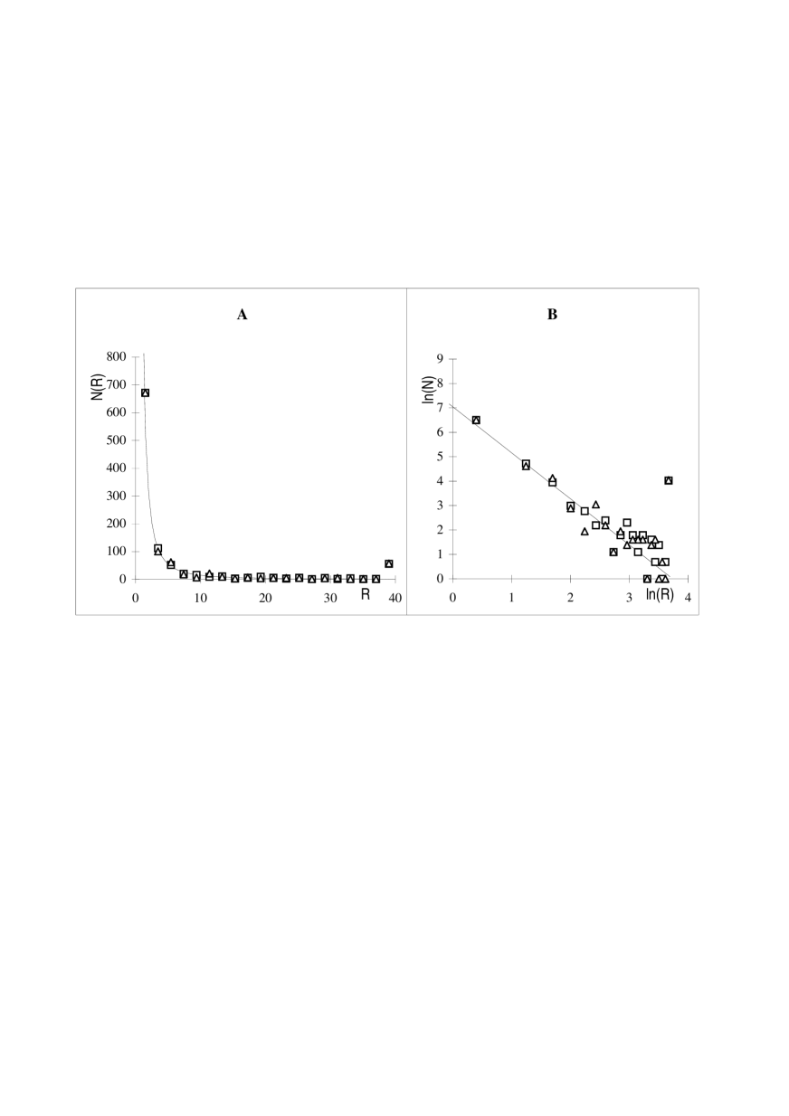
Figure 2: Circle-size distributions of two computer generated circle coverings. (a) Normal scale. (b) Double logarithmic scale. The full line is the average best fit.

The circle size distribution is characterized by one peak at the maximum radius and by a fast increment towards the minimum radius. The linear trend of the distribution, in the region of small radii ($R<R_{Max}/5$), shown in the double logarithmic scale (fig.(2b) ), suggests a power law $N(R)\propto R^{-\alpha}$. The best-fit estimation for the exponent give $\alpha=1.84\pm 0.16$ (squares) and $\alpha=1.92\pm 0.19$ (triangles), with confidence factors respectively equal to $93\%$ and $92\%$.

A power law for the sizes distribution was analytically predicted in the previous paragraphs and in app.A. The best–fit values of the exponents $\alpha$ are in good agreement with the theoretical predictions for the case of disordered maximum circle–packing.

5 Structures formed by condensed tin droplets

Figure (3) is a SEM micrograph of Sn drops condensed on a hot, flat alumina substrate. The system have been prepared evaporating the tin in high vacuum on a substrate heated at a temperature higher than the tin melting point [33, 25]. After cooling at room temperature, one has a stable system of packed tin drops. The size-distribution of such a system was studied using SEM micrographs of magnifications 10 and 20 $K\propto$. The micrographs were digitalized with a scanner. On each image an internal rectangular perimeter was defined and the drops inside and on the bound perimeter were encircled with circles of the same size of the surface occupied by the drop. The size distribution of these circles was studied. The boundary effects were taken into account counting 1/2 the circles crossing an edge of the perimeter and counting 1/4 the circles containing a vertex of the bound-perimeter. In fig.(4) the sizes-distributions for three different samples are reported in normal and double logarithmic scales. The three samples were deposited respectively with 2.5 $g/m^{2}$ (triangles), 2.8 $g/m^{2}$ (squares) and 3.2 $g/m^{2}$ (diamonds). The biggest drops have sizes of about $1000nm$, whereas the smallest (measurable) drop-sizes are $50nm$. The number of drops encircled per each micrograph was about 2000-2500. The distribution is characterized by rather uniform drop sizes in the region of large radii and by a fast increment, as a power law, towards the smallest radii.

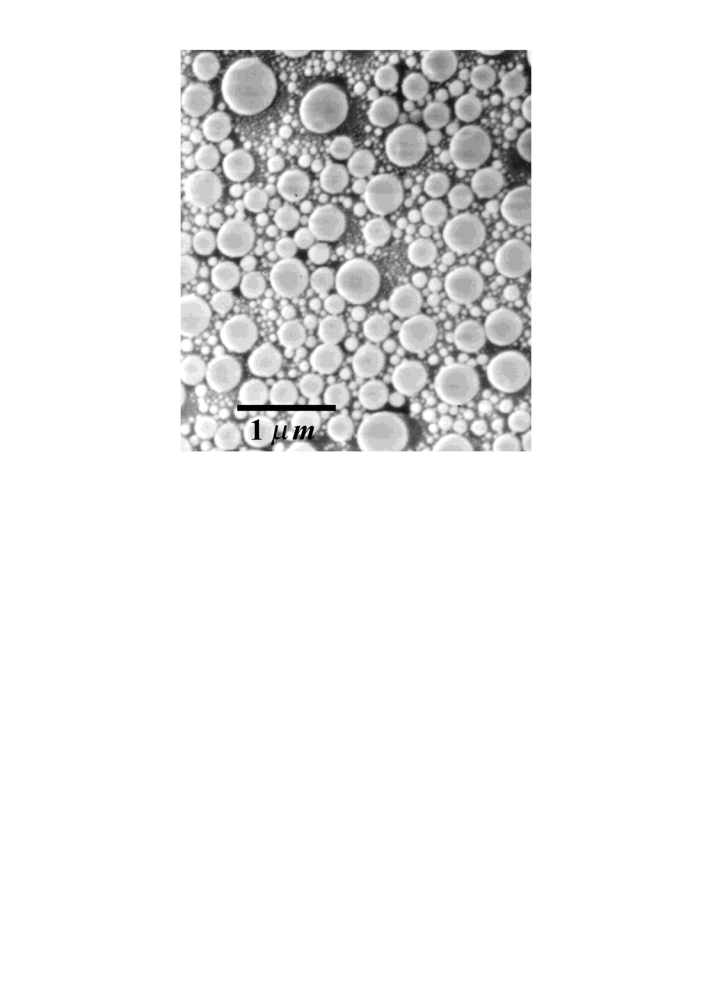
Figure 3: SEM micrograph of a “breath figure” generated by tin drops deposited on a hot alumina substrate.

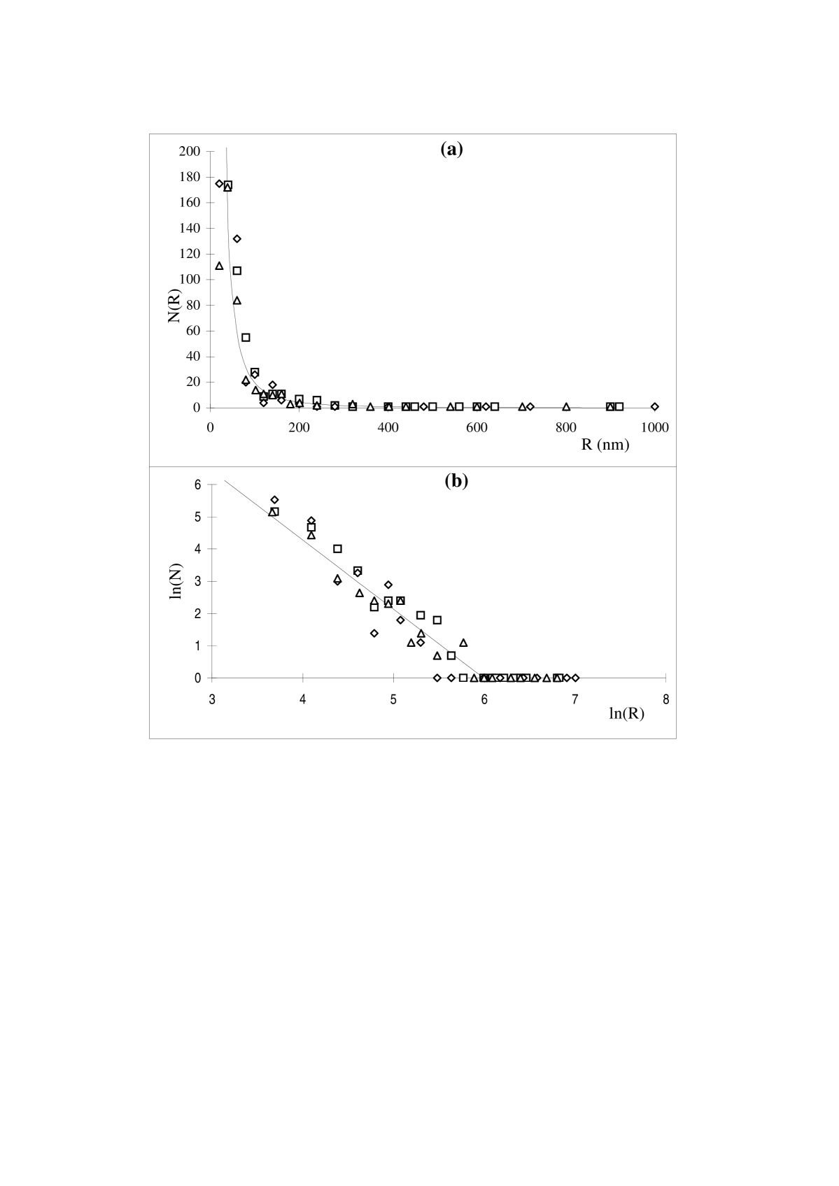
Figure 4: Size distribution of the tin drop diameters for three different samples. (a) normal scale; (b) double logarithmic scale. In ordinates, N(R) is the number of drops per $\mu m^{2}$. The full line is the average best fit.

Typically, one drop nucleates on a preferential centre and grows supported by condensation. This independent growth stops when the drop touch another surrounding drop. At this point, the two drops melt together and the formed new drop –eventually– melts with other surrounding drops in a chain of coalescence events. The coalescence leads to a new drop with volume equal to the sum of the volumes involved in the coalescence phenomena. This new drop occupies a surface lower than the sum of the surfaces occupied by the original drops. It follows that the coalescence mechanism liberates space on the substrate. On this surface the nucleation, growth and coalescence phenomena can start again. The final structure is therefore a consequence of a very complicated process which involve many body phenomena [10]. Nevertheless the formation of the final structure can be investigated adopting a simple point of view.

The system of quenched drops showed in fig.(3) is apparently similar to the systems studied, analytically and numerically, in the previous paragraphs. This similarity is not only apparent: the nucleation, growth and coalescence mechanism leads to systems where the drops occupies the maximum possible surface and have the biggest sizes, compatibly with the coalescence that prevents the drops overlapping. The system evolves through self–similar configurations where the size distribution is, at any time, the maximum packing distribution.

The similarity between this two systems is confirmed by the drop size distribution: in the region of little radii the distribution follows a power law $N(R)\propto R^{-\alpha}$ with exponent $\alpha\simeq 2$. The best–fit give $\alpha=1.96\pm 0.13$ (triangles in fig.(4) ), $\alpha=2.05\pm 0.11$ (squares) and $\alpha=2.1\pm 0.23$ (diamonds), with confidence factors respectively equal to $94\%$, $95\%$ and $87\%$. These values are in accordance with the analytical predictions and strongly suggests that the system morphogenesis is ruled by the mechanism of the maximum circle-packing.

In the region of big radii ($R\simeq R_{Max}>500\;nm$) the drops have a rather uniform sizes. This region of uniform sizes is the memory of the first stage of the deposition where the drops grow independently. Indeed, in this stage the relative volumes of the drops are proportional to the sizes of the Voronoi cell constructed around the drop centers [34], and a rather uniform distribution is expected. In fig.(4) this uniformity at $R\simeq R_{Max}$ is not particularly manifest since the number of drops in this region is little in comparison with the number of small drops ( for example in a sample deposited with about 3 $g/m^{2}$, one has about 10 drops per $\mu m^{2}$ of about $0.1\mu m$ and 1 drop per $\mu m^{2}$ of $1\mu m$). Despite the fact that their number is little, the big drops cover a large amount of surface and contain the main part of the volume deposited (using the same example reported above, it is straightforward to see that the big drops cover an area 10 times larger and occupy a volume 100 times larger than the small drops). Note that, a peak at $R_{Max}$ is present also in the computer simulations. A deviation from the maximum packing law in the region close to $R_{Max}$ is not in contradiction with the theoretical predictions. The analytical result $N(R)\propto 1/R^{\alpha}$, concerns only the asymptotic limit of the distribution ($\nu\rightarrow\infty$ i.e. $R/R_{Max}\rightarrow 0$) where the system is supposed to be scale–invariant.

Studies reported in literature [10, 11, 12, 13, 14, 15, 16, 17], show that the system of condensed drops evolve in time increasing the drop sizes, decreasing the drops number and maintaining constant the coverage. In the systems of tin drops here studied, the coverage have been experimentally found in the range 60% to 65% [22], [25]. A small value of the coverage (typically in breath figures is equal about 55% [15]) is a consequence of coalescence that continuously liberates space. Consider a configuration of three external drops of radius $R_{0}$ and one interstitial drop of radius $R_{1}$. The collapse of these four drops into one trough coalescence liberates a certain amount of surface. The fraction of area liberated (Area occupied by the drops after coalescence/ Area occupied before coalescence) is slightly dependent on the packing strategy. It is equal to $32\%$ if the four drops are all “kissing” each other and equal to $35\%$ in the case of disordered maximum packing ($R_{0}/R_{1}=x\simeq\sqrt{3}$). The presence of other interstitial drops that participate to the coalescence phenomena reduces the previous values within $1\%$. Starting with an initial –hypothetical– coverage of $100\%$, the coalescence reduces the coverage to $68\%$ and $65\%$ in the two cases discussed above. These values are close to the coverage experimentally observed. Note that these values are scale invariant and depends only on the local configurations of drops (i.e. on the packing strategy). The scale invariance implies that the fraction of area liberated by coalescence is independent of the drops radii (i.e. independent of the amount of tin deposited) thus constant during the deposition.

6 Conclusions

Circle–covering is a good model–system for many two dimensional natural cellular system where the plane is filled in the most efficient way compatibly with the cell shapes and sizes. It has been found (§2, §3 and app.A) that polydisperse circles packed in a dense way, have a size distribution that follows the general law $N(R)\propto R^{-\alpha}$. This distribution is a consequence of the scale–invariance in the packing strategy. The range of variability of the exponent have been calculated. We have obtained a maximum value of $\alpha_{Max}=2$ for the general disordered case, where the circles are arranged at random following the only constraint of non overlapping. The minimum value has been estimated $\alpha_{min}\simeq 1$ and corresponds to an approximate solution for the Apollonian packing (§2.1 and §3), and to an exact solution for the “hexagonal” filling model (app.B).

These results, obtained for two dimensional circle packing, have been extended to packing of spheres in spaces of arbitrary dimension (§3.1). We found that, in $D$–dimensional spaces, the size distribution of densely packed $D$–spheres follows –as in 2D– a power law $N(R)\propto R^{-\alpha}$. In this generalized case, the maximum value of the exponent is $\alpha_{Max}=D$ and is associated with disordered packings. The minimum value is associated with the packings of tangents $D$–spheres. For $D=3$, this value have been estimated equal to $\alpha=2.2$ for the Apollonian case, whereas for the hexagonal filling model we found $\alpha=1.26$.

Computer simulations of two–dimensional circle–packing confirm the analytical predictions: in the disordered case the size–distribution follows a power law with exponent $\alpha\simeq 2$ (see §4).

The formation of breath figures have been interpreted in terms of circles packing regulated by coalescence (§5). The mechanism of formation of this figures is very complicated since it is a dynamic system where the evolution involves many–body phenomena. On the other hand, the structures formed by the drops instant by instant have strong similarities with the structures generated by packing circles. In particular, the size distribution in the region of little radii, follows the same power law as the disordered, dense circle-packing with exponent $\alpha\simeq 2$. The coverage, evaluated through the fraction of area liberated by coalescence in a system of drops that follows the maximum packing distribution, is in agreement with the experimental observation.

Acknowledgments

The author wish to thank Rodolfo Botter for the help given for the samples preparation, the microstructural characterization and for the useful discussions. The author thanks F. Saya and P. Pozzolini for the measurements of the drop–sizes distributions. Part of the ideas reported in this paper have been originally developed in the author’s PhD thesis which have been written under the bright supervision of Prof. D. Beruto. Finally, the author thanks Nicolas Rivier for the useful discussions.

Appendix A Size-distribution and covering strategies

In the second and third paragraphs we found that the size distribution of densely packed circles follows a power law (eq.(11) ) where the exponent $\alpha$ is related to the topological properties of the Dodds network and to the parameter $x$ (eq.(12) ). This is a general result where the only a-priori hypothesis is the existence of a Dodds network with convex cells (this condition can be considered as the definition of dense packing). In this appendix we generalize these results using an approach which doesn’t needs the definition of the Dodds network.

Consider a covering procedure which fills the available space with non overlapping circles starting from the circles of bigger sizes $R_{Max}$ and then gradually reducing the sizes $R_{\nu}<R_{Max}$ in order to fill the interstitial spaces. The number of circles introduced at any covering step and the relative sizes depend on the covering procedure. In the second paragraph we pointed out that the scaling condition implies that the number of circles inserted at any covering step grows as a geometrical progression $N_{\nu}\propto a^{\nu}$ and the size of the circles decreases as a geometrical progression $R_{\nu}\propto R_{0}/x^{\nu}$. As a consequence the size distribution results a power law $N(R_{\nu})\propto R_{\nu}^{-\alpha}$ with exponent

$$\alpha={\displaystyle\ln a\over\ln x}\;\;\;\;\;.$$ (23)

In the case of dense packing (i.e. when it is possible to define a Dodds network with convex cells) we found $a=\langle z\rangle/2$ (eq.(22) ) and the bound $x>\sqrt{\langle z\rangle/2}$ (eq.(10) ).

More generally one can construct the Delaunay triangulation with the centre of the circles as vertices. This triangulation is always well defined and (for an infinite system) the average connectivity is $\langle z\rangle=6$. Different packing strategies differentiates in the number, the sizes and the positions of the new vertices (i.e. the new circles) to insert. From a topological point of view, there are only two position where the centre of the new circles can be placed: inside a triangle or on an edge (the centre on a vertex is forbidden by the condition of non overlapping). Suppose that the packing procedure places a new circle with probability $p$ inside a given triangle and with probability $q$ on a given edge of the Delaunay triangulation. If $V_{\nu}$ is the number of vertices (i.e. of circles) at the covering stage $\nu$, it is easy to prove (following the same arguments of §2) that at the next stage this number is

$$V_{\nu+1}=(1+2p+3q)V_{\nu}\;\;\;.$$ (24)

From relation (24) follows immediately that the number of circles grows as a geometrical progression ($N_{\nu}=V_{\nu}\propto a^{\nu}$) with coefficient $a=(1+2p+3q)$.

The argument used in §2 to find the lower bound on the parameter $x$ (eq.(10) ) can be directly extended to the present case. One gets $x>\sqrt{a}$, which, substituted in (23), gives the upper limit $\alpha_{Max}=2$.

The Apollonian covering is a particular example of the covering procedure here discussed. In this case one has $p=1$, $q=0$ and $x\simeq 2.9$, which gives $\alpha\simeq 1$.

Appendix B Hexagonal and triangular filling models

Following the work of Bidaux et al. [19], let us describe two simple circle-covering problems where the exponent $\alpha$ can be calculated exactly. Originally these models have been proposed as simplified geometrical problems to estimates two bounds for the fractal dimension in the Apollonian packing. In the present work these two models are presented as good examples of circle-covering which do not necessarily corresponds to approximations of the Apollonian case.

Let us start with one triangle. In the first model (triangular), one insert a new triangle with vertices in the mean point of the edges of the original triangle. In this way the original triangle is divided in 4 identical triangles which are similar to the original. Then, one insert a circle inside the central triangle and iterate the procedure on the three external triangles. At the beginning one starts with 1 circle, at the first step one insert 3 new circles, at the $\nu^{th}$ step the number of new circles inserted is $3^{\nu}$. The parameter $a$ (see. app.A) is then equal to 3. The ratio $x$ can be easily derived by observing that the triangles are all similar and that at each step of the sequence the sizes of the edges are reduced by a factor 2. Consequently one has $x=2$. Substituting the parameters $a$ and $x$ into eq.(23) one gets the exponent $\alpha=\ln 3/\ln 2\simeq 1.58$.

In the second model (hexagonal) one inscribe first an hexagon with vertices which are dividing in three equal part the edges of the original triangle. Then a circle is inscribed inside the hexagon and the procedure is iterated on the three remaining external triangles. As before one obtains $a=3$, whereas the scale factor is $x=3$. By substituting into eq.(23) we get the exponent $\alpha=1$.

Note that, if one use equilateral triangles the coverage $\theta$ (Area covered by the circles/ Area of the original triangle) can be calculated exactly. One has $\theta=\pi/(3\sqrt{3})\simeq 0.6$ for the triangular model and $\theta=\pi/(2\sqrt{3})\simeq 0.9$ for the hexagonal. These value can be increased by inserting new triangles in the free interstices between the circles and iterating the procedure.

References

- [1] See, for example, in Physics of Granular Media, edited by D. Bideau and J. Dodds (Nova Science Publisher, New York, 1991).
- [2] E. Guyon, S. Roux, A. Hansen, D. Bideau, J.P. Troadec and H. Crapo Rep. Prog. Phys 53,373-419 (1990).
- [3] J.A. Blackman and A. Wilding. Europhys. Lett. 16, 115-120 (1991).
- [4] J.A. Blackman and A. Marshall. J. Phys. A 27, 725-740 (1994).
- [5] J. P. Troadec, A. Gervois, C. Annic and J. Lemaitre, J. Phys. I France 4, 1121-32 (1994).
- [6] H. J. Hermann, G. Mantica and D. Bessis. Phys. Rev. Lett. 65, 3223-3226 (1990).
- [7] S.S. Manna and H. J. Hermann. J. Phys. A 24, L481-L490 (1990).
- [8] D. W. Boyd, Mathematica 20, 170 (1973).
- [9] B. B. Mandelbrot, The fractal Geometry of Nature, §18 (W.H. Freeman and Company, San Francisco1982).
- [10] D. Beysens and M. Knobler Phys.Rev.Lett. 57, 1433-1436, (1986).
- [11] B.J.Briscoe and K.P. Galvin Phys.Rev.A 43, 1906-1917, (1990).
- [12] D. Fritter, C. M. Knobler and D.A. Beysens Phys.Rev.A 43, 2858-2869 (1990).
- [13] C. M. Knobler and D. Beysens Europhys. Lett. 6, 707-712 (1988).
- [14] F. Family and P. Meakin, Phys. Rev. Lett. 61, 428-431 (1988). M. Klob, Phys. Rev. Lett. 62, 1699 (1989). F. Family and P. Meakin, Phys. Rev. Lett. 62, 1700 (1989).
- [15] B. Derrida, C. Godreche and I. Yekutieli, Phys. Rev.A 44, 6241-6251 (1991)
- [16] D. Beysens, C.M. Knobler and H. Schaffar, Phys. Rev. B 41, 9814-9818 (1990)
- [17] D. Fritter, C. M. Knobel, D. Roux and D. Beysens, J. Stat. Phys. 52, 1447-1459 (1988).
- [18] Y. Bouligand, J. Phys. Paris 33, 525-547 (1972).
- [19] R. Bidaux, N. Boccara, G. Sarma, L. de Seze, P. G. de Gennes and O. Parodi, J. Phys. Paris 34, 661-672 (1973).
- [20] H.S.M. Coxeter. Introduction to Geometry. (J. Wiley and Sons, New York, 1961).
- [21] T. Aste, Ph.D. thesis, Politecnico di Milano, Milano (1994).
- [22] P.Pozzolini, thesis, University of Genova, Genova (1994).
- [23] F. Saya, thesis, University of Genova, Genova (1995).
- [24] T. Aste, R. Botter, D. Beruto, C. Ciccarelli, M. Giordani and P. Pozzolini, Sensors and Actuators B 18-19, 637 (1995).
- [25] T. Aste, R. Botter and D. Beruto, Sensors and Actuators B (1995), (to appear).
- [26] J.A. Dodds, J. Colloid. Interface Sci. 77, 317-327 (1980).
- [27] D. Bideau, A. Gervois, L. Oger and J.P. Troadec, J. Physique 47, 1697-1707 (1986).
- [28] F. Soddy, Nature 137, 1021 (1936).
- [29] H.S.M. Coxeter Aequationes Mathematicae 1, 104-121 (1968).
- [30] R. Mosseri and J.-F. Sadoc, in Geometry in Condensed Matter Physics, edited by J.-F. Sadoc (World Scientific, Singapore 1990).
- [31] T. Gosset, Nature 139, 62 (1937).
- [32] N. Rivier, Private communication.
- [33] G. Sberveglieri, G. Faglia, S. Groppelli, P. Nelli and A. Taroni, Sensors and Actuators B, 721-726 (1992)
- [34] P. A. Mulheran, proceedings of Patras euroconference on complex materials, 23 (Patras, 1995).