We find analytical solutions to the Cahn-Hilliard equation for the dynamics of an interface in a system with a conserved order parameter (Model B). We show that, although steady-state solutions of Model B are unphysical in the far-field, they shed light on the local dynamics of an interface. Exact solutions are given for a particular class of order-parameter potentials, and an expandable integral equation is derived for the general case. As well as revealing some generic properties of interfaces moving under condensation or evaporation, the formalism is used to investigate two distinct modes of interface propagation in systems with a metastable potential well. Given a sufficient transient increase in the flux of material onto a condensation nucleus, the normal motion of the interface can be disrupted by interfacial unbinding, leading to growth of a macroscopic amount of a metastable phase.

PACS numbers: 64.60.My, 05.07.Ln, 64.60.Qb

1 Introduction

The kinetics of phase ordering is a central topic in nonequilibrium statistical physics. Much of our understanding is based on theories that describe one or more slowly-varying density (or order parameter) variables, governed by a local Langevin equation [1]. In general, the density variable(s) evolve(s) systematically in response to a driving force, which is a derivative of the underlying free energy functional, with some mobility (characterized by the Onsager matrix). On top of this are noise terms whose magnitude is fixed by requiring that the Boltzmann distribution is a stationary state of the dynamics. The nature of the Onsager mobility depends on the kind of ordering involved; specifically we must distinguish conserved order parameters from nonconserved ones. In the conserved case, the density in some region can change only by diffusive transport across its boundary; its time derivative is therefore the divergence of a current. This is not the case for nonconserved order parameters, which can change locally in direct response to the driving force.

The low temperature (noise-free) limit is usually considered appropriate for the study of phase ordering kinetics, in which a system is prepared far from equilibrium and then allowed to evolve. For example, a uniform high-temperature phase can be quenched into a region where it is either locally or globally unstable with respect to separation into two macroscopic phases. Local instability leads to spinodal decomposition [2]; if the system is locally stable, phase separation proceeds by a nucleation and growth mechanism [3]. In either case, the governing equation for phase separation of a conserved scalar order parameter is the Cahn-Hilliard equation [4]:

$$\frac{\partial\rho}{\partial t}=\mbox{\boldmath$\nabla$}\cdot\left(\Gamma\mbox{\boldmath$\nabla$}\left\{\frac{df}{d\rho}-K\nabla^{2}\rho\right\}\right).$$ (1)

As explained in Section 2, $K$ is the square-gradient coefficient in a free energy expansion, which treats the order parameter, $\rho$, as slowly varying; $\Gamma$ is the mobility. Note that in principle Cahn-Hilliard theory can accommodate an arbitrary form of $f(\rho)$, which is the free energy density for a homogeneous state. (In particular, it does not assume that $f$ is a polynomial in the order parameter $\rho$, as would be assumed in the time dependent Landau-Ginzburg theory of dynamics close to a critical point [5].) Indeed, the approach should be qualitatively applicable even if $f(\rho)$ consists of the lower envelope of several unrelated functions representing phases of different symmetry. The free energy near a liquid-solid transition is of this form, for example, with $\rho$ the material density. This assumes only that, whatever other order parameters distinguish the various phases (such as crystallinity), these can relax quickly and hence that the rate-limiting process for the phase ordering is transport of $\rho$. It is conventional, in equation 1, to treat $K$ as a constant (independent of $\rho$). We do this in what follows, although it might be a dangerous assumption when $f$ is a composite function as just described. With this caveat, equation 1 will be relevant at long times and large distances if the other order parameters are nonconserved.

In this paper, we therefore consider the phase ordering problem for relatively general forms of $f(\rho)$, where $\rho$ is a concentration variable. We assume this is the only conserved order parameter, thereby ruling out systems with significant concentration deviations in more than one species, and also ruling out consideration of heat transport. This latter restriction might be severe in (say) metallurgical applications, but not for soft condensed matter systems (such as colloidal suspensions) which are our main interest. Indeed, for many such systems the latent heats of phase changes are entirely negligible [6].

Our work is motivated by the desire to understand better the role of metastable phases in the kinetics of phase separation. That such a role exists has been long acknowledged: for example, the “Ostwald rule of stages” [7] asserts that a system will progress from an unstable to a stable state, not directly, but by a sequence of steps through any intervening metastable states that may be present. In the area of metallurgy, there is an extensive folklore on the subject [8]. Here we aim at a more fundamental understanding, based on a direct analysis of the Cahn-Hilliard problem. For the most part, we work in one space dimension.

Specifically, we shall focus on steady-state solutions of the Cahn-Hilliard equation, in which interfaces between phases move with constant velocities. This approach appears at first paradoxical, since the diffusive nature of the transport rules out true constant-velocity solutions when conserved order parameters are present. (Indeed the basic scaling of lengths in diffusive transport is with $t^{1/2}$ whereas constant velocities would imply linear scalings.) However, as we discuss later, significant physical insights can be gained by viewing the interfacial motion as a quasi-steady process. A broadly comparable analysis, for nonconserved dynamics (where true steady-state motion is possible) has been given recently by Bechhoefer et al. [9, 10, 11]. These authors showed that under sufficient supercooling (or, equivalently in a ferromagnetic system, sufficient applied field) the interface between two stable coexisting phases could become dynamically unstable toward “splitting”. The splitting instability results in a macroscopically thick slab of a metastable phase appearing between the two stable phases, which can then grow.

One of the main questions we address here, and in a companion paper [12] is whether the same scenario is possible for the conserved order parameter case. In this paper we show that, although there is no mathematically direct analogue of the splitting instability found by Bechhoefer et al., a sufficient transient flux from the less dense to the more dense stable phase can indeed cause interfacial splitting. We also argue that the split mode will be maintained so long as the supersaturation of the less dense phase is sufficiently large. In the companion paper [12] we study the long time limit in which the interfaces become sharp on the scale of their separation, and give a more detailed discussion of the critical supersaturation required to sustain the split mode at long times. That paper also contains a discussion of experimental evidence, involving colloid-polymer mixtures [13], which suggests that the onset of the split mode might be connected with the observation of arrested crystallization, beyond a threshold of supersaturation, in the transition from a colloidal fluid to a colloidal crystal. A brief account of these ideas is given in [14].

The rest of this paper is organized as follows. In Section 2 we recall the Cahn-Hilliard equation and discuss the conditions under which a one-dimensional treatment should suffice. In Section 3 we formulate the quasi steady-state form of the Cahn-Hilliard equation, paying careful attention to the boundary conditions that are required to make the solution physically meaningful. An exact solution is described for a piecewise quadratic potential $f(\rho)$, with piecewise constant mobility. In Section 4 we describe in more detail the properties of the solution, focusing on the case where $f(\rho)$ shows a metastable minimum of intermediate density. We argue that there is no critical velocity above which the interface between stable phases ceases to have a steady-state solution (in contrast to the nonconserved case) and in Section 5 we show explicitly that such an “unsplit” mode of interface motion is linearly stable. In Section 6, however, we show that a split interface, should one arise, can also be dynamically stable under appropriate conditions. We discuss qualitatively the nature of the (large) perturbation required to cause splitting. Section 7 summarizes our conclusions. Appendix A provides some details of the exact solution for the piecewise quadratic case, whereas in Appendix B we derive an exact integral representation of the steady-state solution for general potentials, thereby confirming and extending some of the earlier results.

2 The Cahn-Hilliard Equation

Consider a system characterized by one conserved, scalar order parameter, such as local mass density, in a part of the phase diagram where two-phase coexistence is the equilibrium state. If the system is far from criticality, and is initially out of equilibrium, then its evolution towards equilibrium obeys Model B, described by equation 1 (the Cahn-Hilliard equation), which is derived as follows. Let the free energy of the system be a functional $F[\rho]$ of the order parameter $\rho(\mbox{\boldmath$x$})$. Then the chemical potential is defined by the functional derivative,

$$\mu=\frac{\delta F}{\delta\rho}$$

($\mu$ can thereby depend on gradients of $\rho$, as well as $\rho$ itself). Currents in Model B are induced by gradients of the chemical potential:

$$\mbox{\boldmath$j$}=-\Gamma\mbox{\boldmath$\nabla$}\mu$$

where the constant of proportionality, $\Gamma$ is the Onsager mobility, which may be a function of $\rho$. Since the order parameter is conserved, its time-derivative is given by a continuity equation,

$$\frac{\partial\rho}{\partial t}=-\mbox{\boldmath$\nabla$}\cdot\mbox{\boldmath$j$}.$$

Let the free energy functional be of the form

$$F[\rho]=\int d^{d}x\left\{f(\rho)+\mbox{$\frac{1}{2}$}K(\mbox{\boldmath$\nabla$}\rho)^{2}\right\}.$$

The form of the bulk free energy density (or ‘order-parameter potential’) $f$, and the value of $K$, are system-dependent. Let the system in question be initially homogeneous at a non-equilibrium value of $\rho$, between two minima in $f$; i.e. within a two-phase coexistence region of the phase diagram. For definiteness, let $\rho$ be initially close to the low-density minimum in $f$. Small fluctuations initially induce the evolution of $\rho$ towards equilibrium. Early stages of the evolution proceed by nucleation, if $f$ is convex at the given value of $\rho$, or by spinodal decomposition, if concave. This stage of the dynamics is not addressed here. By whatever process, domain walls (interfaces) soon form. If surface tensions are neglected (legitimate when typical interfacial radii of curvature are large, which we assume), subsequent motion of a wall is driven by diffusion from the far-field. The local profile of the wall changes on a shorter time scale than the far-field gradients which determine the flux onto the wall, simply because of the difference in length scales: while typical distances between interfaces are proportional to $t^{1/2}$, the characteristic width an interface remains of the order of $\sqrt{K/(d^{2}f/d\rho^{2})}$ at all times. Therefore, although typical inter-wall distances vary with time, intra-wall dynamics (concerning the local density profile of an interface) soon become approximately steady-state, with a quasi-constant input flux.

These local interface dynamics are concerned with the movement of a $(d-1)$-dimensional wall in a $d$-dimensional space, translating normal to itself. Hence, if curvature and surface-tension effects are ignored, the problem becomes one-dimensional; the Cahn-Hilliard equation then reduces to

$$\frac{\partial\rho}{\partial t}=\frac{\partial}{\partial x}\left(\Gamma(\rho)\frac{\partial}{\partial x}\left(\frac{df}{d\rho}-K\frac{\partial^{2}\rho}{\partial x^{2}}\right)\right).$$

In the next Section, we show how to find steady-state solutions of this equation for a piecewise-quadratic potential.

3 Exact Steady-State Solution

Let us transform to a frame moving at velocity $v$, in which the position coordinate is

$$s\equiv x-vt,$$

and introduce the notation $f_{n}(\rho)\equiv(d/d\rho)^{n}f(\rho)$. Demanding that the time derivative vanishes in this frame, we find that a steady-state solution $\rho(s)$ to the Cahn-Hilliard equation, travelling at velocity $v$ satisfies

$$\rho^{\prime\prime\prime\prime}-\frac{f_{2}}{K}\rho^{\prime\prime}-\frac{v}{K\Gamma}\rho^{\prime}=\frac{f_{3}}{K}\rho^{\prime 2}+\frac{1}{\Gamma}\frac{d\Gamma}{d\rho}\left(\frac{f_{2}}{K}\rho^{\prime}-\rho^{\prime\prime\prime}\right)\rho^{\prime}$$ (2)

which is a third-order ordinary differential equation in $\rho^{\prime}$($\equiv d\rho/ds$). If $\Gamma$ and $f_{2}$ are both independent of $\rho$ then the right-hand side vanishes and the left-hand side becomes linear and homogeneous in $\rho^{\prime}$. So the problem is (at least) piecewise-soluble for a piecewise-quadratic potential $f(\rho)$, with piecewise-constant mobility $\Gamma$. Such a model is actually fairly versatile, and we therefore explore it in detail.

At discontinuities in our piecewise-constant $f_{2}$ and/or $\Gamma$, the solutions for the separate pieces must respect certain matching conditions. Specifically, the current must be continuous so that $\nabla\cdot j$ remains finite; the chemical potential must be continuous to avoid infinite currents; and continuity of the gradient of $\rho$ is required to avoid infinities in the chemical potential. These three conditions are sufficient to fix the constants of integration for the above third-order equation in $\rho^{\prime}$. Subsequent integration to find $\rho$ gives rise to an additional arbitrary constant, which is fixed by demanding continuity of $\rho$ itself. The full solution is given in detail in Appendix A. For each piece of the potential, this solution has the form

$$\rho^{\prime}(s)=\sum_{j=1}^{3}A_{j}e^{\omega_{j}s}$$ (3)

where the constants $A_{j}$ and $\omega_{j}$ depend on $f_{2}$, $K$, $\Gamma$ and $v$.

In addition to the matching conditions (which fix some of the constants arising in equation 3 from the division of $f(\rho)$ and $\Gamma(\rho)$ into pieces) boundary conditions are required, to select a specific solution to the differential equation. The correct choice and interpretation of these boundary conditions are not trivial; we discuss them carefully before proceeding further. The case of interest

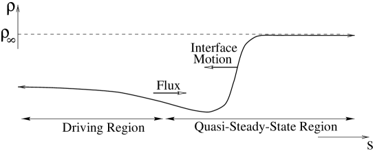
Figure 1: Schematic diagram of the system. Density $\rho$ is plotted against distance $s$. On the right of the figure, a high density domain has formed, for which $\rho\rightarrow\rho_{\infty}$ as $s\rightarrow+\infty$. On the low density side of the interface, the region for which the quasi-steady-state approximation holds meets the ‘driving region’, which becomes depleted as material condenses onto the interface.

(depicted in figure 1) is where a region of the high-density phase has formed, and is growing by condensation from the supersaturated low-density phase. (Note that, throughout this paper, the high-density phase is depicted on the right of the diagrams, and therefore grows by leftward motion of the interface. The opposite convention is adopted in Refs. [12] and [14].) The interface is to be modelled in isolation, so the high-density phase is semi-infinite. Two boundary conditions arise from this: that the density (and hence chemical potential) asymptotes to a constant value, $\rho_{\infty}$ as $s\rightarrow+\infty$ (say), and that the flux asymptotes to zero in this limit. We may now either regard $v$ in equation 2 as a given constant and then, from integration, deduce the conditions at the other boundary, or $v$ may be seen as an eigenvalue which is set by further boundary conditions. In any case, at the second boundary a flux is required (to induce motion), and this implies a gradient in the chemical potential. Hence it does not make sense to put this boundary at $s\rightarrow-\infty$, as $\mu$ would be infinite here; instead the left-hand boundary must be at some finite position. This raises two possible worries: that the thermodynamic limit cannot be taken since the model is of a finite system, and that steady-state solutions cannot be found in a finite system. The interpretation which resolves these difficulties is as follows. The left-hand boundary is at a finite distance from the interface, and moves with the interface. It is not in fact the edge of the system, but simply the point at which the behaviour ceases to be quasi-steady-state. The part of the system to the left of this boundary, which does not solve the steady-state equation, may be referred to as the ‘driving region’, since it is responsible for supplying the quasi-constant flux and chemical potential to the propagating interface, by non-steady-state diffusive depletion of material. In summary, a specific solution to the steady-state equation is fixed by the asymptotic value of $\rho$ in the limit $s\rightarrow+\infty$ and by the values of the chemical potential and flux at some (rather ill-defined) position to the left of the interface, where the steady-state region meets the driving region.

4 Properties of the Solution

One important qualitative observation, noticeable on graphs (such as those discussed in section 4.1) of the exact steady-state solution calculated in Appendix A, is that the characteristic width of the interface always decreases as the speed of condensation (or equivalently the incident flux) increases. In Appendix B, it will be shown, to first order in $v$, that this is a generic result. A second qualitative result, found below (Section 4.2), is that steady-state solutions exist at all velocities $v$. This holds even when an intermediate metastable well is present in the order parameter potential; accordingly (and in contrast to the case of a nonconserved order parameter [9]) there is no critical velocity above which the interface must split. Both of these results have implications for the formation of metastable phases.

4.1 Form of the Interfacial Profile

Before discussing splitting, we show some typical numerical results for a steadily moving interface, in a system where a metastable phase is possible. Consider a system in which $f(\rho)$ contains a metastable well at a density between that of the growing high-density phase, and the supersaturated low-density phase. A piecewise-parabolic form for such a potential is shown in figure 2a. (Metastability requires

Figure 2: (a) A piecewise-quadratic three-well potential $f(\rho)$, for which all relevant parameters are given. Well number 2 is metastable. (b) The density profile of an equilibrium interface for the above potential. Regions are labelled in which the density corresponds to wells 1, 2 and 3 of the potential. (c) Density profile of an interface moving at velocity $-0.02K\Gamma$ for the same potential, and constant mobility $\Gamma$. Notice that region 2 is narrower than in the equilibrium case.

that the middle well is above the common tangent to the other two wells.) Let the low, intermediate and high density wells be referred to as 1, 2 and 3 respectively. We may define the order parameter $\rho$ (chosen as a scaled, relative density) to be $\pm 1$ at the minima corresponding to phases 1 and 3, and take their free energy densities $f(-1),f(+1)$ to be equal. (This choice involves no loss of generality, since, as is well-known [15], adding a linear term to the free energy density ($f\rightarrow f+a\rho+b$) has no effect on the solutions of the Cahn-Hilliard equation.) Steady-state interface profiles for this system are given in figure 2b for $v=0$ (i.e. the equilibrium wall) and (in fig. 2c) for $v=-0.02K\Gamma$. In each case the mobility $\Gamma$ is constant throughout the system. Negative-$v$ solutions are of greatest interest, since they describe the condensation of material from a supersaturated region onto a growing domain, and are therefore central to phase-ordering dynamics. Notice that both solutions shown have an inflection at the density of the metastable phase 2. Without forming a macroscopic amount of the metastable phase, the interface takes advantage of the local minimum in free energy by having extra material at this density. Region 2 is noticeably narrower in figure 2c (for condensation) than in figure 2b (the equilibrium profile).

4.2 Existence of Solutions for an Unsplit Interface for All $v$

We are interested in whether such a steady-state interface might split into two parts, the 1-2 part of the interface propagating faster than the 2-3 part, analogously to the ‘dynamic splitting instability’ [9] which can arise in the dynamics of a non-conserved order parameter in a three-welled potential. In the non-conserved case, a critical velocity exists, above which there exists no steady-state solution for the propagation of a 1-3 interface; instead a macroscopic amount of the metastable phase 2 must be created between a pair of moving (1-2 and 2-3) interfaces.

In comparing the conserved and non-conserved dynamics however, an important distinction should be borne in mind. In the non-conserved case, the velocity of each interface is controlled by an external field, which adds a linear term to the potential. (Indeed, to obtain a dynamic splitting instability in the non-conserved case, the field must cause the potential in the middle well to fall below that of one of the others.) In the conserved case, however, linear terms in the potential are irrelevant; instead, the velocity is controlled by the boundary conditions. We now present an argument showing that the unsplit propagation mode exists for all velocities in this case. (The argument is not limited to the case of piecewise quadratic potentials.)

First, note that equation 2 may in principle be integrated spatially, from right to left, for a given $v$ and $\rho_{\infty}$, to find the value of $\rho$ at any point. This could fail to produce a solution for a three-well potential, only if the resultant profile $\rho(s)$ fails to span all three wells due to the presence of a minimum in the function $\rho(s)$. This would occur whenever the given value of $v$ was above the critical value. However, such turning points in $\rho(s)$ do not arise in the steady-state solutions. This follows from the expression for the chemical potential

$$\mu=\frac{df(\rho)}{d\rho}-K\frac{\partial^{2}\rho}{\partial x^{2}}\;.$$

To see why, consider first the equilibrium interface profile, for which $\mu$ is a constant. Clearly, this spans all three wells. Any solution of negative $v$ (describing condensation) must have a higher chemical potential than the equilibrium value, at any given point on the interface where $\rho<\rho_{\infty}$, because there is a steady flux onto the high-density phase. Hence, for any given value of $\rho$, it follows from the above expression for $\mu$ that the curvature of $\rho(s)$ must be more negative than for the equilibrium profile. So no minimum exists in $\rho(s)$. This argument also holds if $\rho_{\infty}$ is greater than the equilibrium value, since there is still no minimum to the $v=0$ solution in this case. The argument may even be extended to the case where $\rho_{\infty}$ is below the equilibrium value so that the $v=0$ solution exhibits a minimum. So long as this static solution spans all three wells, negative $v$ solutions with the same asymptote must also do so, since their curvature at any given value of $\rho$ is more negative. Hence there is no critical velocity for condensation.

5 Stability of the Solutions

Having established the existence of solutions corresponding to unsplit interfacial propagation at all velocities $v$, we now show that these solutions are stable against linear perturbations. (The argument below is restricted to piecewise quadratic $f(\rho)$.)

Let the field $\rho(x,t)$ obey the full Cahn-Hilliard equation of motion, and be written as

$$\rho(x,t)=\rho_{0}(x,t)+\varepsilon(x,t)$$

where $\rho_{0}(x,t)$ is a solution of the steady-state equation, and $\varepsilon$ is initially small. Differentiating with respect to time gives

$$\frac{\partial\varepsilon}{\partial t}=\frac{\partial}{\partial x}\left(\Gamma\left.\frac{\partial\mu}{\partial x}\right|_{\rho_{0}+\varepsilon}\right)-\left.\frac{\partial}{\partial x}\left(\Gamma\frac{\partial\mu}{\partial x}\right|_{\rho_{0}}\right)$$

where

$$\mu|_{\rho_{0}+\varepsilon}=\mu|_{\rho_{0}}+\varepsilon f_{2}(\rho_{0})-K\frac{\partial^{2}\varepsilon}{\partial x^{2}}+{\cal O}(\varepsilon^{2}).$$

For the exact solutions calculated in Appendix A, $f_{2}$ and $\Gamma$ are both piecewise constant. It follows that, on any piece of this solution, a small perturbation $\varepsilon$ about the solution obeys the linearized equation of motion

$$\frac{\partial\varepsilon}{\partial t}=\Gamma f_{2}\frac{\partial^{2}\varepsilon}{\partial x^{2}}-\Gamma K\frac{\partial^{4}\varepsilon}{\partial x^{4}}.$$

In Fourier space, writing

$$\varepsilon(x,t)=\int_{-\infty}^{\infty}\tilde{\varepsilon}(q,t)e^{iqx}\,dq$$

the equation of motion becomes

$$\frac{\partial\tilde{\varepsilon}(q,t)}{\partial t}=-q^{2}\,(\Gamma f_{2}+\Gamma Kq^{2})\,\tilde{\varepsilon}(q,t).$$

In any well in the potential, the coefficient $-q^{2}(\Gamma f_{2}+\Gamma Kq^{2})$ is negative for all $q$. So all Fourier modes of a small perturbation, about any piece of the solution in a quadratic well, decay exponentially with time. Also, since the pieces of the solution must always obey the matching conditions at cusps in the potential, the solution as a whole is stable, when all continuous parts of the potential are convex (as is the case, for instance, in the potential of figure 2a). Furthermore, in any concave part of the potential, solutions are stable with respect to perturbations of shorter wavelength than $2\pi\sqrt{K/(-f_{2})}$. Hence, so long as the spatial distance over which the interfacial profile spans a concave part of the potential is less than $2\pi\sqrt{K/(-f_{2})}$, the solution will be stable. It is obviously true that the equilibrium interface profile satisfies this linear stability criterion. As stated previously, we have observed solutions, for interfaces moving due to condensation, to be narrower than the equilibrium interface (and proved it to first first order in $v$ in Appendix B); hence they too are linearly stable.

Although this completes the argument, it is useful to have a conceptual picture of the mechanisms giving rise to this stability. Consider once more the profile in figure 2c of a moving interface for a potential with a metastable middle well. A perturbation such as that shown by the dashed line in figure 3 may be considered as a small change in $s$ at constant

Figure 3: Density profile of a steadily moving interface (solid line) and the result of a perturbation in the direction of the arrows (dashed line) which has increased the width of the region occupying the metastable middle well of the potential. The result is a more negative curvature in the position labelled A, and more positive curvature at B.

$\rho$, rather than vice versa. The perturbation shown is tending to separate the 1–2 part of the interface from the 2–3 part, thus widening the metastable region. Notice that this makes the curvature more negative on the part of the interface labelled ‘A’, and more positive at ‘B’. So the chemical potential is increased at A and reduced at B, thus enhancing the flux onto the 2–3 part of the wall. So the 2–3 part of the wall will catch up with the leading 1–2 part, and steady-state motion will be restored. This negative feedback mechanism is responsible for the linear stability of an unsplit interface.

It is worth noting, in addition, that numerical solutions of the Cahn-Hilliard equation have been performed, using a three-well potential, and have confirmed that 1–3 interfaces may propagate stably, even at large values of $v$.

6 Local Dynamics of a Split Interface

It was shown above that steady motion of a 1–3 interface, spanning the intermediate metastable well, is linearly stable. Hence a 1–3 interface, once formed, continues to propagate in the absence of large perturbations. Such perturbations may however arise, especially in the early stages of interface formation (including the dynamics prior to the time at which the Cahn-Hilliard equation becomes a good approximation). Therefore, let us consider the situation whereby a large slab of metastable phase 2 has formed, by whatever mechanism, so that the 1–2 and 2–3 interfaces are separated by a distance large compared with the scale $\sqrt{K/f_{2}}$ set by the curvature term in the free energy. Such a situation is depicted in figure 4, in which various quantities are defined: the interface separation $\Delta x$, the two interface velocities $v_{1}$ and $v_{2}$, the fluxes into the 1–2 interface, $j_{1}$, and between the interfaces, $j_{2}$ (both of which are taken to be approximately constant over the spatial regions of interest), and four densities $\rho_{A}$, $\rho_{B}$, $\rho_{C}$ and $\rho_{D}$. Let us

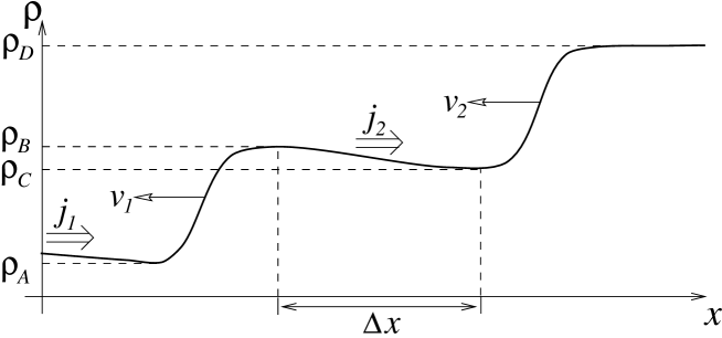
Figure 4: Density profile of a system in which 1–2 and 2–3 interfaces are separated by a distance $\Delta x$. The interfaces are travelling with velocities $v_{1}$ and $v_{2}$ respectively. Densities $\rho_{A}$, $\rho_{B}$, $\rho_{C}$ and $\rho_{D}$ and fluxes $j_{1}$ and $j_{2}$ are also defined in the figure.

introduce a further approximation, as follows. We assume that the interfaces are moving sufficiently slowly that the densities $(\rho_{A},\rho_{B})$ and $(\rho_{C},\rho_{D})$ on either side of each are approximately the values that would arise at coexistence of the two given phases, in the absence of the third. These pairs of values of $\rho$ may be found from the bulk free energy density by the usual double-tangent construction, as shown in figure 5 (which also shows the construction for the globally stable binodal values $(\rho_{\alpha},\rho_{\beta})$ for 1–3 phase coexistence). In principle the double tangent construction is subject to small corrections due to interface motion; these are calculated, for completeness, in Appendix C but we neglect them here.

6.1 Growth or Collapse?

The time evolution of such an interface is not strictly a question of steady-state (or even quasi-steady-state) dynamics. Accordingly we give only a brief discussion, and leave a fuller exploration of this interesting problem to the companion paper [12] (see also [14]). The basic issue is whether the slab of metastable phase grows or shrinks.

When curvature is small, as is the case between the interfaces, the Cahn-Hilliard equation is well approximated by the diffusion equation, $\dot{\rho}=D\nabla^{2}\rho$, with the diffusivity given by $D=\Gamma f_{2}(\rho)$ which is approximately constant given that $\rho$ does not vary much. ($D$ is exactly constant in a quadratic potential well of fixed $\Gamma$.) Notice in figure 5 that the inequality $\rho_{B}>\rho_{C}$ is a necessary result of the metastability of well 2. Hence, since the diffusion equation governs the inter-wall region, $j_{2}$ is positive. Thus flux flows onto the 2–3 interface, contributing positively to $v_{2}$ and negatively to $v_{1}$. So, the effect of $j_{2}$ is to reduce $\Delta x$, as would be expected for the dynamics of a metastable phase. If phase 2 is to grow, the constant flux $j_{1}$ into the system must be sufficiently large to make $|v_{1}|>|v_{2}|$. Invoking the diffusion approximation, and the linearity of the function $\rho(x)$ in phase 2, the condition for growth of the metastable phase (rather than recombination of the 1–3 interface) becomes

$$j_{1}>D\frac{(\rho_{B}-\rho_{C})}{\Delta x}\left(1+\frac{\rho_{B}-\rho_{A}}{\rho_{D}-\rho_{C}}\right).$$ (4)

Figure 5: Figure demonstrating the double-tangent construction to find the stable binodal densities $(\rho_{\alpha},\rho_{\beta})$ and the metastable binodal densities $(\rho_{A},\rho_{B})$ and $(\rho_{C},\rho_{D})$ in a three-well potential. This potential can be converted to the form of fig.2 by adding or subtracting a linear term ($f\to f+a\rho+b$), and then both shifting the origin of $\rho$, and rescaling it.

When this condition is satisfied, a ‘split’ mode of interfacial propagation can arise, which is fundamentally different from the propagation of an unsplit 1–3 interface in a number of respects. The most important distinction is that now, if $j_{1}$ is held constant, the width of the metastable region, $\Delta x$ grows without limit. In contrast, in a stable 1–3 interface, $\Delta x$ remains bounded. Indeed, in the equilibrium ($v=0$) interface, $\Delta x$ is of the order of the characteristic interfacial width $\sim\sqrt{K/f_{2}}$, and at higher speeds, $\Delta x$ becomes smaller. Accordingly there is an upper bound on $\Delta x$ close to the equilibrium value (although not equal to it, since unsplit propagation is resumed after a small, positive perturbation in $\Delta x$).

Another qualitative difference between the split and unsplit modes of propagation is their response to a perturbation. It was demonstrated in Section 5 that increasing the width $\Delta x$ of the metastable region led to an increase in the flux though it, resulting in a negative feedback mechanism. On the other hand, if the interface is split, and therefore non-monotonic and containing a well-developed region in which diffusive motion is dominant over curvature-induced motion, increasing $\Delta x$ reduces the gradient in region 2. This reduces $j_{2}$, and causes the 2–3 interface to lag still further behind the 1–2 wall. So the corresponding feedback in split interface motion is positive. It follows that, at constant $j_{1}$, there is a barrier (in configuration space) to the formation of an unsplit interface, but once this barrier is crossed, such an interface will remain split indefinitely.

6.2 Selection of Split or Unsplit Mode

It has been shown that (at least for piecewise-quadratic potentials) the propagation of an unsplit interface is locally stable, and that, given sufficient input flux, the split interface mode is also “stable” (in the sense of remaining split indefinitely). The question arises of which mode of evolution will be selected in a given system, and how it might be possible to change from one to the other. Clearly in a real system, the flux input to an interface is not constant. Normally, in late-stage evolution, it is a diminishing function of time. One might conclude from this that the criterion for growth of the split mode (equation 4) must at some point be violated. However, this criterion becomes easier to satisfy as $\Delta x$ increases. The ultimate fate of a split interface in fact depends on supersaturation: this is described in the companion paper [12].

The problem of how to ‘unbind’ a 1–3 interface is somewhat clearer: a large transient increase in input flux is required, to overcome the negative feedback mechanism described in Section 5. There is presumably some critical value of $\Delta x$ at which the feedback switches from negative to positive and the interface splits. The transient increase in flux must be sufficient to separate the leading (1–2) part of the interface from the trailing part by this critical amount, before the interface can deliver a restorative increase in flux to region 3 by curvature-induced motion. If the transient increase of input flux is insufficient, and the 1–3 interface adjusts to the new higher speed, the criterion for unbinding it becomes more stringent (since higher-speed interfaces are narrower, and hence both further from the critical value of $\Delta x$, and ‘stiffer’ in terms of the negative feedback mechanism). Since fluxes tend to decrease with time during late-stage phase-ordering, a transient increase in flux, sufficient to unbind a 1–3 interface, is most likely to occur during the early stage dynamics (nucleation or spinodal decomposition). These dynamics are not quasi-steady-state, and we do not discuss them further here. But it is interesting that, whenever metastable phases are possible, the details of these early stage dynamics can determine the gross features (split vs. unsplit mode) of phase separation at much later times.

Finally, in the context of mode selection, a useful distinction can be drawn between two types of interfacial binding/unbinding. The type described above can be called “curvature unbinding” – the process whereby $\Delta x$ becomes large compared to $\sqrt{K/f_{2}}$. In the companion paper [12] (see also [14]) we study “diffusive unbinding” which is linked to the evolution of $j_{1}$ (treated above as an externally imposed parameter). In Ref. [14], we also report numerical results which show that curvature unbinding certainly does occur, within the Cahn-Hilliard equation, at least for some parameter values and some initial conditions. These include cases (such as an initial step function wall between phases 1 and 3) which, though strongly perturbed from the equilibrium profile, are definitely not unbound to begin with.

7 Conclusion

It is often assumed that steady-state solutions of the Cahn-Hilliard equation (Model B), for the phase ordering dynamics of a conserved order parameter, are unphysical and therefore uninteresting. In this article we have shown that such solutions shed light on the local dynamics of interfaces, so long as care is taken to interpret the boundary conditions correctly. Exact solutions were found for the case of any piecewise-quadratic order parameter potential and piecewise-constant mobility; these are locally stable. For the most general case of arbitrary bulk free energy density and mobility as functions of mass density $\rho$, a systematic expansion scheme was derived (Appendix B) to solve Model B for a moving interface. Using this scheme, it can be shown (to at least first order in $v$) that an interface contracts when moving under condensation, and expands during evaporation. If a metastable phase exists, whose density is intermediate to the two stable phases, a moving interface between the stable phases is still locally stable with respect to small perturbations at all speeds, but may be ‘split’ by a large, transient increase in the flux of condensing material, and thereafter exhibit a qualitatively different mode of propagation. Such a transient disturbance is most likely to arise in the early stages of nucleation and growth. The split mode of interface motion results in the formation of a macroscopically large amount of the metastable phase and relies on a sufficiently large flux of condensing material being maintained. A companion paper [12] (see also [14]), discusses further the implications of these findings for the growth rates of competing stable and metastable domains during the phase-ordering process.

8 Acknowledgements

This work was supported by EPSRC Grant No. GR/K56025. We thank Wilson Poon for a series of illuminating discussions.

Appendix A Exact Solution of the Steady-State Equation for Piecewise-Quadratic Potential

Equation 2 is now solved to find $\rho(s)$ for any piecewise-quadratic potential $f(\rho)$ and piecewise-constant mobility $\Gamma(\rho)$. Between discontinuities in $f_{1}$, $f_{2}$ or $\Gamma$, $\rho(s)$ solves the equation

$$\rho^{\prime\prime\prime\prime}-a\rho^{\prime\prime}-b\rho^{\prime}=0$$

where $a=f_{2}/K$ and $b=v/(K\Gamma)$. The solution is

$$\rho^{\prime}(s)=\sum_{j=1}^{3}A_{j}e^{\omega_{j}s}$$

for some constants $A_{j}$, fixed by the boundary conditions and matching conditions. The constants $\omega_{j}$ are the three roots of the cubic equation

$$\omega_{j}^{3}-a\omega_{j}-b=0$$

which is solved, for $27b^{2}<4a^{3}$, by

$$\omega_{1} = 2\sqrt{\frac{a}{3}}\sin\left(\frac{\sigma-2\pi}{3}\right)$$

$$\omega_{2} = 2\sqrt{\frac{a}{3}}\sin\left(\frac{\sigma}{3}\right)$$

$$\omega_{3} = 2\sqrt{\frac{a}{3}}\sin\left(\frac{\sigma+2\pi}{3}\right)$$

where

$$\sigma\equiv-\arcsin\sqrt{\frac{27b^{2}}{4a^{3}}}.$$

If $27b^{2}>4a^{3}$, the solutions may be written in terms of the real quantities $\alpha\equiv(\frac{1}{2}b+\frac{1}{2}\sqrt{b^{2}-\frac{4}{27}a^{3}})^{1/3}$ and $\beta\equiv(\frac{1}{2}b-\frac{1}{2}\sqrt{b^{2}-\frac{4}{27}a^{3}})^{1/3}$ as

$$\omega_{1} = \alpha+\beta$$

$$\omega_{2} = -\mbox{$\frac{1}{2}$}(\alpha+\beta)+i\mbox{$\frac{\sqrt{3}}{2}$}(\alpha-\beta)$$

$$\omega_{3} = \omega_{2}^{*}$$

All that remains to be found is the vector of coefficients $\mbox{\boldmath$A$}\equiv\left(\begin{array}[]{c}A_{1}\\ A_{2}\\ A_{3}\end{array}\right)$ for each piece. This is fixed by assigning values to $\rho^{\prime}$, $\rho^{\prime\prime}$ and $\rho^{\prime\prime\prime}$ at the right-hand boundary of each section, which may be re-defined as the origin of $s$ by multiplying $A$ by an appropriate exponential factor. From the equation for $\rho^{\prime}(s)$, it follows that

$$\mbox{\boldmath$A$}=\left(\begin{array}[]{ccc}1&1&1\\ \omega_{1}&\omega_{2}&\omega_{3}\\ \omega_{1}^{2}&\omega_{2}^{2}&\omega_{3}^{2}\end{array}\right)^{-1}\left(\begin{array}[]{c}\rho^{\prime}(0)\\ \rho^{\prime\prime}(0)\\ \rho^{\prime\prime\prime}(0)\end{array}\right).$$

The vector of derivatives of $\rho$ is determined, from the solution in the neighbouring piece, by the matching conditions given in Section 3, where it was stated that the gradient, chemical potential and flux must all be continuous. That is, the quantities $\rho^{\prime}$, $(K\rho^{\prime\prime}-f_{1})$ and $(K\rho^{\prime\prime\prime}-f_{2}\rho^{\prime})\Gamma$ are continuous. These quantities can be calculated from the neighbouring solution, given the value of $s$ at which it meets the discontinuity (say $s=s_{1}$). If the discontinuity (in the mobility or potential) is at a value $\rho=\rho_{1}$, then $s_{1}$ is given by inverting the equation $\rho(s_{1})=\rho_{1}$ which, unfortunately cannot in general be done analytically. (However, the inversion is always possible for the reasons explained in Section 4.2.) Hence one numerical step is required in the solution. (Of course the special case of a double-well potential, with just one cusp discontinuity, is completely soluble analytically, since the arbitrary origin of $s$ can be put at the cusp of $f(\rho)$.)

Finally, the boundary condition that $\rho\rightarrow\rho_{\infty}$ as $s\rightarrow+\infty$ results in the solution for the highest density section: $\mbox{\boldmath$A$}=\left(\begin{array}[]{c}-(\rho_{\infty}-\rho_{1})\>\omega_{3}\\ 0\\ 0\end{array}\right)$ and hence
$\rho^{\prime}(s)=-(\rho_{\infty}-\rho_{1})\>\omega_{3}\>e^{\omega_{3}s}$ for $s>0$, and $\rho(0)=\rho_{1}$.

Appendix B Integral Solution of Cahn-Hilliard

In Section 4, the assertion was made that interfaces generically contract when moving under condensation. This result and its converse (that interfaces expand during evaporation) will be derived now, using a systematic expansion of steady-state solutions of the Cahn-Hilliard equation in powers of the interface velocity $v$. As previously, we consider the one-dimensional Cahn-Hilliard equation in a frame moving at velocity $v$, in which distance is measured by the coordinate $s$; the order parameter $\rho$ asymptotes to a finite constant $\rho_{\infty}$ as $s\rightarrow+\infty$. However, in contrast to the analysis in Section 3 and Appendix A, no particular form will be assumed for the order parameter potential $f(\rho)$, and likewise the mobility $\Gamma(\rho)$ will be an arbitrary function.

B.1 Inversion of Variables

It is convenient to invert the equation so that $\rho$ becomes the independent variable, and the equation is solved for $s$. This means that the unspecified potential $f(\rho)$ and mobility $\Gamma(\rho)$ are now functions of the independent variable. Henceforth let the curvature constant $K$ be set to unity without loss of generality. (This is equivalent to measuring time in units of $K$ and length in units of $\surd K$.) After inversion, the full, one-dimensional Cahn-Hilliard equation in a moving frame may be written

$$\frac{\partial s}{\partial t}\,\,=\,\,\frac{\partial}{\partial\rho}\left[\left(\frac{\partial s}{\partial\rho}\right)^{\!-1}\!\!\Gamma\>\frac{\partial^{2}}{\partial\rho^{2}}\left\{\frac{1}{2}\left(\frac{\partial s}{\partial\rho}\right)^{\!-2}\!\!-f\right\}\right]-v.$$

Clearly (as is well-known) adding a linear term to the potential $f(\rho)$ has no effect.

B.2 Integration of the Steady-State Equation

Let us now set the time derivative to zero in this moving frame, and integrate once with respect to $\rho$, to obtain the steady-state equation

$$\Gamma(\rho)\left(\frac{ds}{d\rho}\right)^{\!-1}\frac{d^{2}}{d\rho^{2}}\left\{\frac{1}{2}\left(\frac{ds}{d\rho}\right)^{\!-2}\!\!-f(\rho)+\lambda\rho+c\right\}\,\,=\,\,(\rho-\rho_{\infty})v$$

where the arbitrary linear term $-(\lambda\rho+c)$ has been explicitly added to $f(\rho)$. Note that the constant $\lambda$ is equal to the chemical potential in the asymptotically flat region: $\lambda=\mu(\infty)$ (remember $\mu$ is non-uniform in a moving interface). It can be confirmed that $-v\rho_{\infty}$ is the correct constant of integration, given that the left-hand side of the above equation is simply the flux $j$.

Let us define $h(\rho)\equiv ds/d\rho$, so that $1/h=\nabla\rho$. Then integrating with respect to $\rho$, we find

$$\frac{d}{d\rho}(\mbox{$\frac{1}{2}$}h^{-2}-f+\lambda\rho+c)=v\int\frac{(\rho-\rho_{\infty})h}{\Gamma}\,d\rho+\mbox{const.}$$

It is easy to confirm that the left-hand side of this equation is the chemical potential, measured with respect to the value at $\rho_{\infty}$. Now consider the factors in the integrand. As $\rho\rightarrow\rho_{\infty}$, $(\rho-\rho_{\infty})$ tends to zero linearly, while it is expected (and confirmed in the special case of appendix A) that $h(\rho)\rightarrow\infty$ logarithmically. Hence the integrand vanishes as $\rho\rightarrow\rho_{\infty}$. So the constant in the above equation is zero, and we have

$$\frac{d}{d\rho}(\mbox{$\frac{1}{2}$}h^{-2}-f+\lambda\rho+c)=-v\int_{\rho}^{\rho_{\infty}}\frac{(\rho^{\prime}-\rho_{\infty})}{\Gamma(\rho^{\prime})}h(\rho^{\prime})\,d\rho^{\prime}.$$

Let us henceforth absorb the terms $\lambda\rho+c$ into the definition of $f(\rho)$. (That is, the arbitrary linear part of $f(\rho)$ is defined so that the potential has zero value and gradient at $\rho_{\infty}$.) Integrating by parts once gives the final result

$$h(\rho)=\frac{1}{\sqrt{2f(\rho)}}\left\{1-\frac{v}{f(\rho)}\int_{\rho}^{\rho_{\infty}}\frac{(\rho_{\infty}-\rho^{\prime})(\rho^{\prime}-\rho)}{\Gamma(\rho^{\prime})}h(\rho^{\prime})\,d\rho^{\prime}\right\}^{-\frac{1}{2}}$$ (5)

Notice that the Cahn-Hilliard equation, in its differential form, is fourth order, but that this integral representation of the steady-state equation contains only one integration.

If $h(\rho)$ is written as a power-series in $v$, then the binomial in equation 5 may be expanded, and the formula iterated to produce a systematic series approximation for $h$, to arbitrarily high powers of the velocity. The power-series expansion of the steady-state solution $s(\rho)$ is then obtained by integration as:

$$s(\rho)=\int h(\rho)\,d\rho.$$

Clearly the origin of $s$ (and hence the constant of integration) is arbitrary.

B.3 First-Order Correction to Interfacial Width

This method is now applied to find the first-order correction to the width $\Delta s$ of a moving interface, defined as the distance between two points on the interface at which the densities have certain fixed values $\rho_{1}$ and $\rho_{2}$ (which could be the densities of the two maxima in a three-well potential, for example). It transpires that

$$\Delta s = \Delta s_{0}+cv+{\cal O}(v^{2})$$

$$\mbox{where}\,\,\Delta s_{0} = \int_{\rho_{1}}^{\rho_{2}}\frac{d\rho}{\sqrt{2f(\rho)}}$$

$$\mbox{and}\,\,\,\,c = \frac{1}{4}\int_{\rho_{1}}^{\rho_{2}}d\rho\,f(\rho)^{-\frac{3}{2}}\int_{\rho}^{\rho_{\infty}}d\rho^{\prime}\,(\rho_{\infty}-\rho^{\prime})(\rho^{\prime}-\rho)\Gamma(\rho^{\prime})^{-1}f(\rho^{\prime})^{-\frac{1}{2}}.$$

This last equation expresses the rate of change of width of the interface with velocity, $c$ in terms only of the two functions which characterize the physics of the system; the bulk free energy density $f(\rho)$ and the mobility $\Gamma(\rho)$. All factors in the integrands of this expression are positive over the ranges of integration, so $c$ is positive. Negative values of $v$ correspond to growth of the asymptotically flat, dense region by condensation, and positive values correspond to evaporation. So, without assigning any special properties to the functions $f$ and $\Gamma$, it has been shown that the interface contracts ($\Delta s<\Delta s_{0}$) during condensation and expands during evaporation.

As mentioned at the end of Section 4, $\rho_{\infty}$ may vary from its equilibrium value (i.e. the density at which phase 3 coexists in equilibrium with phase 1 for a three-well potential). In the present section, a formalism has been developed by which the solution for a moving interface is expanded about the $v=0$ solution. Does this allow for variation in $\rho_{\infty}$? The answer is ‘yes’ because there is in fact a whole family of $v=0$ solutions with different values of $\rho_{\infty}$, of which the equilibrium solution is just one member. The equilibrium solution is the special member of this family for which $\rho$ asymptotes to a finite constant as $s\rightarrow-\infty$, rather than growing exponentially (either positive or negative) and thus remaining curved and having unphysical boundary conditions at $s\rightarrow-\infty$. But, for our purposes, the whole family may be used since, as discussed in Section 3, the left-hand boundary is not put at negative infinity.

Appendix C Correction to the Double-Tangent Construction for a Moving Interface

The double-tangent construction illustrated in figure 5 gives the equilibrium densities of two coexisting phases. Recall its elementary derivation as follows [8]. In a uniform part of the system of volume $V$, containing $N$ particles, the local density is $\rho=N/V$, and the free energy is $F=fV$. From these two simple relations, and the definitions of chemical potential $\mu=(\partial F/\partial N)_{V}$ and pressure $P=-(\partial F/\partial V)_{N}$, it follows that $f=\mu\rho-P$, which is the equation of a straight line on a plot of $f$ versus $\rho$, with gradient $\mu=f^{\prime}(\rho)$ and intercept $-P$. Given that two coexisting phases have equal chemical potentials and pressures, it follows that the straight lines tangent to $f(\rho)$ at the respective coexistent densities have equal gradients and intercepts. Hence they are the same line.

Consider now the non-equilibrium case of an interface in uniform motion at velocity $v$. By continuity, the flux at any point on the interface is $j=-(\rho_{\infty}-\rho)v$. In model B, $\nabla\mu=-j/\Gamma$. Hence, integrating across the interface, the difference in chemical potential between the dense, asymptotically uniform phase at positive infinity, and any given point $A$ is

$$\Delta\mu\equiv\mu(\infty)-\mu(A)=v\int_{A}^{\infty}\frac{(\rho_{\infty}-\rho)}{\Gamma}dx$$

from which the equilibrium result follows for $v=0$.

Now let us consider the local quantity $P\equiv\mu\rho-f$ (which reduces to the usual definition of pressure in a homogeneous system). With this definition,

$$\nabla P=\rho\nabla\mu-K\nabla^{2}\rho\nabla\rho.$$

Using again the above expression for $\nabla\mu$, and integrating gives

$$\Delta P\equiv P(\infty)-P(A)=\left[-\frac{1}{2}K\left(\frac{\partial\rho}{\partial x}\right)^{2}\right]_{A}^{\infty}-\int_{A}^{\infty}\frac{\rho j}{\Gamma}dx.$$

If the curvature part of the chemical potential is small at point $A$, this expression for the pressure difference becomes

$$\Delta P=-\mbox{$\frac{1}{2}$}K\left[\left(\frac{j}{\Gamma f^{\prime\prime}}\right)^{2}\right]_{A}^{\infty}-\int_{A}^{\infty}\frac{\rho j}{\Gamma}dx=-\int_{A}^{\infty}\frac{\rho j}{\Gamma}dx+{\cal O}(v^{2}).$$

So the equality of chemical potentials and pressures across a static interface, which gives rise to the double-tangent construction, has the following corrections, to first order in $v$, for a moving interface:

$$\Delta\mu = v\int_{A}^{\infty}\frac{(\rho_{\infty}-\rho)}{\Gamma}\>dx$$

$$\Delta P \approx v\int_{A}^{\infty}\frac{(\rho_{\infty}-\rho)\>\rho}{\Gamma}\>dx.$$

Notice that both corrections depend on the range of integration, i.e. on the position of the point $A$. This is no surprise, since there must be gradients in the pressure and chemical potential outside the interface in order induce motion. Notice also that both coefficients of $v$ are positive, so $\Delta\mu$ and $\Delta P$ are of the same sign as $v$. This is negative for condensation and positive for evaporation. So, as expected, during condensation the pressure difference and chemical potential difference across an interface are smaller than at equilibrium.

References

- [1] P. M. Chaikin and T. C. Lubensky, Principles of Condensed Matter Physics, Cambridge University Press (1995), chap. 7.
- [2] J. M. Gunton, M. San Miguel and P. S. Sahni, in Phase Transitions and Critical Phenomena, ed. C. Domb and J. L. Lebowitz, Academic Press, London, 1983, vol. 8, ch. 3.
- [3] J. S. Langer in Solids Far from Equilibrium, ed. C. Godrèche, Cambridge University Press (1995), chap. 3.
- [4] J. W. Cahn and J. E. Hilliard, J. Chem. Phys. 28 258 (1958).
- [5] P. M. Chaikin and T. C. Lubensky, Principles of Condensed Matter Physics, Cambridge University Press (1995), chap. 8.
- [6] H. Löwen, Phys. Rep. 237 (1994) 249.
- [7] W. Ostwald, Z. Physik. Chem. 22 286 (1897).
- [8] R. T. DeHoff, Thermodynamics in Material Science, McGraw Hill, New York (1993).
- [9] J. Bechhoefer, H. Löwen and L. S. Tuckerman, Phys. Rev. Lett. 67 (1991) 1266–1269.
- [10] F. Celestini and A. ten Bosch, Phys. Rev. E 50 1836 (1994).
- [11] L. S. Tuckerman and J. Bechhoefer, Phys. Rev. A 46 3178 (1992).
- [12] R. M. L. Evans and W. C. K. Poon, following article.
- [13] W. C. K. Poon, A. D. Pirie and P. N. Pusey, Faraday Discussion 101 65 (1995).
- [14] R. M. L. Evans, W. C. K. Poon and M. E. Cates, cond-mat/9701110.
- [15] A. J. Bray, Advances in Phys. 43 (1994) 357.