Fractional pumping of energy into a ballistic quantum ring.

Abstract

We consider the energy stored in a one-dimensional ballistic ring with a barrier subject to a linearly time-dependent magnetic flux. An exact analytic solution for the quantum dynamics of electrons in the ring is found for the case when the electro-motive force ${\cal E}$ is much smaller than the level spacing, $\Delta$. Electron states exponentially localized in energy are found for irrational values of the ratio $A\equiv\Delta/2e{\cal E}$. Relaxation limits the dynamic evolution and localization does not develop if $A$ is sufficiently close to a rational number. As a result the accumulated energy becomes a regular function of $A$ containing a set of sharp peaks at rational values (fractional pumping). The shape of the peaks and the distances between them are governed by the interplay between the strength of backscattering and the relaxation rate.

Physical properties of mesoscopic systems are governed by quantum interference. Several phenonema of such a nature have been discussed for systems close to equilibrium. Persistent currents in multiply-connected systems[1] as well as universal fluctuations of the conductance are important examples[2]. Coherent dynamics remains crucially important in situations far from equilibrium provided the energy associated with the phase breaking rate is less than the characteristic rate of redistributing electrons in energy space. Consequently, one can expect pronounced mesoscopic behavior even in strongly biased mesoscopic devices, where the dynamics can be effectively tuned by external electric or magnetic fields.

In this paper, we consider an example of such a system, namely a single-channel mesoscopic ring subjected to a nonstationary perpendicular magnetic field, linearly dependent on time. We concentrate on the energy accumulation in such a system. To investigate the role of interference, we take into account electron backscattering from a single potential barrier, embedded in the ring. Tuning the transmission through the barrier by gate potentials one can influence the interference pattern and in this way significantly change the dynamics.

Impure onducting rings have been extensively discussed in connection with energy dissipation in mesoscopic metallic systems. Gefen and Thouless[3, 4] have suggested that disorder leads to a localization of electrons in energy space. Consequently, a time-dependent magnetic flux, $\Phi$, through the ring could induce a (dc) circular current only in the presence of phase breaking processes. This work was continued in Ref. [5] by a numerical analysis of the role of dissipation. A numerical analysis of localization in a dissipation-free impure ring was performed in Ref. [6].

The vanishing of the flux-induced current in an impure dissipation-free ring[3, 4] is drastically different from what happens in a perfect ballistic ring, where a non-equilibrium flux driven current diverges when the dissipation goes to zero. This makes the crucial importance of the backscattering strength clear: By tuning the height of the barrier one can cross over from one regime to the other, and in this way control the pumping of energy into the system. This issue, not addressed in previous work, is the subject of the present paper.

We will show that the scenario of the cross over is as follows. Consider the conductance of the ring, $G$, defined as the ratio between the circulating current and the electro-motive force ${\cal E}=-(1/c){\dot{\Phi}}$ induced in a ring of radius $r_{0}$ by a magnetic field linearly dependent on time. If scattering is strong, $G\propto{\cal E}^{-2}$. As the scattering strength decreases, a set of peaks in the function $G=G({\cal E})$ appears. The peaks correspond to rational values $p/q$ of the quantity $A\equiv\Delta/2e{\cal E}$, where $\Delta=\hbar^{2}N_{F}/mr_{0}^{2}$. Here $N_{F}$ is the number of filled electron states while $m$ is the effective mass. The shape of the peaks and the distances between them are governed by an interplay between the height $V$ of the potential barrier and the relaxation rate, $\nu$, the maximum value of $q$ being determined by the condition $\tau^{q}/q\simeq\hbar\nu/e{\cal E}$. Here $\tau\equiv\exp(-{\cal E}_{c}/{\cal E})$ is the effective amplitude of Zener tunneling through the energy gaps in the electron spectrum, ${\cal E}_{c}=\pi^{2}V^{2}/2\Delta e$. The peak structure near maximum can be described by the interpolation formula

$$g=\tau^{2q}\frac{\hbar\nu\Delta}{(\hbar\nu)^{2}+(e{\cal E}q)^{2}\varepsilon^{2}}+\eta q^{2}\frac{\hbar\nu\Delta}{(e{\cal E})^{2}},\ \varepsilon=A-\frac{p}{q}$$ (1)

Here $g\equiv G/G_{0},\ G_{0}=e^{2}/h$, while $\eta(\varepsilon)$ is a smooth function of $\epsilon$. If $|\varepsilon|\leq\tau^{q}/q^{2}$ the function $\eta\sim 1$, beyond this region it decreases as $|\varepsilon|$ increases. As the barrier becomes more transparent, $\tau\rightarrow 1$, the inter-peak distance (determined by the maximum value of $q$) decreases. Finally, the peaks overlap forming the ballistic-like conductance $g=\Delta/\hbar\nu$.

To understand the result conjectured above let us consider the electron energy levels in the vicinity of the Fermi level, $E_{F}$. Here the energy dispersion can be considered to be linear. In a ballistic ring, one has then two sets of adiabatic energies $E_{l}(\Phi)$ corresponding to clock- and counterclockwise motion (Fig. 1). The sets coincide and scattering from the barrier opens gaps for those flux values where $E_{l}=E_{F}+l\Delta/2,\ l=0,\pm 1,\pm 2,\ldots$. Consequently, the energy pumping into the system by a slowly varying magnetic flux can be mapped to the one-dimensional motion of a quantum particle in the field of periodically placed scatterers (cf. Refs. [3, 4, 6]). Landau-Zener tunneling (with the amplitude $\tau$ introduced above) through the gaps corresponds to forward scattering while reflection from the gaps is similar to backscattering. The important difference from the usual impurity problem is that there is no translational invariance at an arbitrary value of the driving force ${\cal E}$. This invariance is only present for rational values $p/q$ of the dimensionless quantity $A$[6]. In this case we arrive at a super-lattice containing $q$ “impurities” per unit cell. As a result, the motion along the $E$-axis is described by $q$ allowed bands, the “velocity” being $v_{E}\equiv{\dot{E}}\sim\Delta\tau^{q}/t_{0}$ (here $t_{0}\equiv h/e{\cal E}$ is twice the time interval between two sequential Landau-Zener scattering events). Since the upper bound of the Brillouin zone is $4\pi\hbar/q\Delta$, the corresponding bandwidth for motion along the $E$-axis is $W\simeq v_{E}4\pi\hbar/q\Delta\simeq 4\pi\hbar\tau^{q}/t_{0}q$. At rational values $p/q$ of the quantity $A$ the electron rotates around the ring an integer number, $2p$, of times during the time the enclosed magnetic flux changes by $q$ flux quanta. As a result motion along the $E$-axis can be mapped onto motion in a one-dimensional periodic potential, the corresponding eigenstates being extended. If $p/q$ is irrational the motion along the $E$-axis is equivalent to motion in a one-dimensional quasi-periodic potential. It turns out that the corresponding states are then localized (see below) in spite of the fact that there is no real disorder in the system. The localization radius, $R_{loc}$, can be estimated for $A=p/q+\varepsilon,\ |\varepsilon|\ll 1/q$ as follows: In this case the phase mismatch due to finite $\varepsilon$ can be thought of as being due to a quasicassical potential $U(E)=\varepsilon\alpha E$ with $\alpha=8\pi\hbar/\Delta t_{0}$. One can see that a finite $\varepsilon$ gives rise to band bending which creates semiclassical turning points for the propagating modes along the $E$-axis. The localization length is in fact one half of the distance between the turning points produced by the upper and lower band edges, $R_{loc}\simeq W/2\alpha|\varepsilon|=\Delta\tau^{q}/4q|\varepsilon|$. Consequently, the localization time is $t_{\text{loc}}\sim 4R_{loc}/v_{E}\sim t_{0}/q|\epsilon|$.

The manifestation of localization in the energy pumping depends on the product $\nu t_{\text{loc}}$. When $\nu t_{\text{loc}}\gg 1$ localization has not developed and the band picture of energy pumping is relevant. The conductance is estimated as (cf. Ref. [4]) $G=P/{\cal E}^{2}$, where $P$ is the average energy accumulation rate. The quantity $P$, in its turn, is determined as $\nu\delta E\cdot N(\delta E)$. Here $\delta E\sim v_{E}/\nu$ is the energy accumulated by a single state, while $N(\delta E)\sim\delta E/\Delta$ is the number of involved states. It follows that $g\sim\tau^{2q}(\Delta/\hbar\nu)$. If $\nu t_{\text{loc}}\ll 1$, on the other hand, $G$ is determined by hops between intra-band localized states. In this case, $\delta E\sim 2R_{loc}$, and we obtain $g\sim\hbar\nu\Delta\tau^{2q}/(e{\cal E}q\varepsilon)^{2}$. These estimates are consistent with the first term in Eq. (1).

The consideration above are valid if the localization length is greater than the unit cell size, $2R_{loc}\gg q\Delta/2$. In the opposite limit the band picture fails and the velocity is dominated by inter-band transitions. In this case, $\delta E\sim q\Delta,\ N(\delta E)\sim q$, and $g\sim q^{2}\hbar\nu\Delta/(e{\cal E})^{2}$. This estimate corresponds to the second term in Eq. (1).

The following model is employed. The electron system is described by the Hamiltonian

$${\cal H}(t,\varphi)=-\Delta\sigma_{z}\left(i\frac{\partial}{\partial\varphi}+\frac{t}{t_{0}}\right)+{\cal H}_{\text{imp}}(\varphi),\ t_{0}\equiv\frac{ch}{|e|{\dot{\Phi}}}$$ (2)

Here $\sigma_{i}$ are Pauli matrices. We are interested in the current, averaged over the time $t_{0}$,

$$J(t)=\frac{1}{t_{0}}\int_{t-t_{0}/2}^{t+t_{0}/2}dt^{\prime}\,\text{Tr}\,{\hat{\rho}}{\hat{\jmath}}\,\quad{\hat{\jmath}}\equiv e{\dot{\hat{\varphi}}}\,.$$ (3)

The single-electron density matrix, $\hat{\rho}$, is calculated from the equation

$$\frac{\partial\hat{\rho}}{\partial t}=\frac{i}{\hbar}[{\hat{\rho}},{\cal H}]-\nu\left({\hat{\rho}}-f_{0}\bigl{(}{\cal H}(t)\bigr{)}\right),$$ (4)

where $f_{0}$ is the Fermi function. The formal solution of Eq. (4) can be expressed in terms of the evolution operator ${\hat{u}}(t,t^{\prime})$ for the systems described by the Hamiltonian (2),

$${\hat{\rho}}(t)=\nu\int_{-\infty}^{t}dt^{\prime}\,e^{\nu(t^{\prime}-t)}{\hat{u}}(t,t^{\prime})f_{0}\bigl{(}{\cal H}(t^{\prime})\bigr{)}{\hat{u}}^{{\dagger}}(t,t^{\prime})\,.$$ (5)

We are interested in the case of weak scattering, i.e. when the matrix element $V$ of the scattering potential corresponding to a momentum transfer of $\sim 2p_{F}$ is much smaller than the inter-level spacing $\Delta$. In such a situation, the impurity potential is important only in the vicinity of the times when the adiabatic levels for clockwise and counterclockwise motion cross. It creates gaps near the crossing points. Consequently, one can discriminate between intervals of ballistic evolution (duration $\sim t_{0}/2$) and intervals of Landau-Zener scattering. The typical duration of such an interval is $\leq\sqrt{t_{0}\hbar/\Delta}$ (cf. Ref. [8]). Consequently, at $\Delta t_{0}/\hbar\gg 1$ the Landau-Zener scattering is strongly confined within narrow intervals and can be described in terms of the scattering matrix

$${\hat{S}}=\exp(i\theta)\left[\rho\exp(i\xi\sigma_{z})+i\tau\sigma_{x}\right],\ \rho=\sqrt{1-\tau^{2}}$$ (6)

where $\tau$ has been introduced above. It turns out that the physical values of interest here do not depend on the phases $\theta$ and $\xi$. For simplucity we put them equal to zero. The expression for $J$ has the form

$$\frac{J}{J_{0}}=-\tau^{2}+\sum_{m=0}^{\infty}e^{-2{\tilde{\nu}}m}\text{Tr}\,{\hat{T}}^{-m}{\hat{J}}{\hat{T}}^{m}{\hat{\cal F}}\,,$$ (7)

where $J_{0}=e\Delta/\hbar$ is the amplitude of the persistent current, ${\tilde{\nu}}\equiv\nu t_{0}/2$,  ${\hat{T}}=\exp(-i{\hat{\varphi}}){\hat{u}}(t_{0},0)$,

$${\hat{J}} = \frac{1}{t_{0}}\int_{-t_{0}/2}^{t_{0}/2}dt\,{\hat{u}}^{+}(t,0)\sigma_{z}{\hat{u}}(t,0)\,,$$ (8)

$${\hat{\cal F}} = \int_{-t_{0}/2}^{t_{0}/2}dt\,{\hat{u}}^{+}(t,0)\frac{\partial f_{0}\bigl{(}{\cal H}(t)\bigr{)}}{\partial t}{\hat{u}}(t,0)\,.$$ (9)

Here we have employed the relation ${\hat{u}}(t+mt_{0},t^{\prime}+mt_{0})=\exp(im{\hat{\varphi}}){\hat{u}}(t,t^{\prime})\exp(-im{\hat{\varphi}})$ which immediately follows from a similar symmetry property of ${\hat{\cal H}}$.

The problem of calculating the current is reduced to an analysis of the unitary operator $\hat{T}$. Having in mind the periodicity in $\varphi$ of all quantities we introduce the basis

$$|n,s=\pm\rangle\equiv\frac{e^{\pm i(N_{F}+n)\varphi}}{\sqrt{2\pi}}{\bf s_{\pm}},\quad{\bf s_{+}}=\left(\begin{array}[]{c}1\\ 0\end{array}\right),\ {\bf s_{-}}=\left(\begin{array}[]{c}0\\ 1\end{array}\right)\,.$$

In this representation, the operator $\hat{T}$ can be expressed as a direct product of operators acting in $n$ and pseudo-spin ($s$) spaces,

$${\hat{T}}=\rho{\hat{S}}e^{i\pi a\sigma_{z}}\otimes e^{4i\pi a{\hat{n}}}+i\tau\sum_{\pm}{\hat{S}}\sigma_{\pm}\otimes e^{2i\pi a{\hat{n}}}{\hat{R}}_{\pm}e^{2i\pi a{\hat{n}}}\,,$$

where the operators ${\hat{R}}_{\pm}$ and $\hat{n}$ are defined as ${\hat{R}}_{\pm}|n,s\rangle=|n\mp 1,s\rangle$, and ${\hat{n}}|n,s\rangle=n|n,s\rangle,$ and $a$ is the fractional part of the quantity $A$ introduced above, $\sigma_{\pm}=(\sigma_{x}\pm i\sigma_{y})/2$. In the $n,s$-representation the operators ${\hat{J}}$ and ${\hat{\cal F}}$ have the form ${\hat{J}}={\hat{V}}\delta_{n,n^{\prime}}$, ${\hat{\cal F}}={\hat{V}}\delta_{0,n}\delta_{0,n^{\prime}}$, ${\hat{V}}=\tau^{2}\sigma_{z}-\rho\tau\sigma_{y}f.$

It is straightforward to show that the unitary operator $\hat{T}$ has the following properties:

$$\hat{R}_{-}\hat{T}\hat{R}_{+}=e^{-4i\pi a}\hat{T},\,\,\sigma_{y}{\hat{T}}^{*}(-\hat{n})\sigma_{y}=\hat{T}(\hat{n})$$

These result in the following relations between the eigenstates $\mathchoice{{\hbox{\boldmath$\displaystyle\psi$}}}{{\hbox{\boldmath$\textstyle\psi$}}}{{\hbox{\boldmath$\scriptstyle\psi$}}}{{\hbox{\boldmath$\scriptscriptstyle\psi$}}}_{\beta}(n)$ of the operator $\hat{T}$ having eigenvalues $\exp(i\beta)$:

$$\mathchoice{{\hbox{\boldmath$\displaystyle\psi$}}}{{\hbox{\boldmath$\textstyle\psi$}}}{{\hbox{\boldmath$\scriptstyle\psi$}}}{{\hbox{\boldmath$\scriptscriptstyle\psi$}}}_{\beta}(n+1) = \mathchoice{{\hbox{\boldmath$\displaystyle\psi$}}}{{\hbox{\boldmath$\textstyle\psi$}}}{{\hbox{\boldmath$\scriptstyle\psi$}}}{{\hbox{\boldmath$\scriptscriptstyle\psi$}}}_{\beta-4\pi a}(n)\,,$$ (10)

$$\sigma_{y}\mathchoice{{\hbox{\boldmath$\displaystyle\psi$}}}{{\hbox{\boldmath$\textstyle\psi$}}}{{\hbox{\boldmath$\scriptstyle\psi$}}}{{\hbox{\boldmath$\scriptscriptstyle\psi$}}}_{\beta}^{*}(-n) = \mathchoice{{\hbox{\boldmath$\displaystyle\psi$}}}{{\hbox{\boldmath$\textstyle\psi$}}}{{\hbox{\boldmath$\scriptstyle\psi$}}}{{\hbox{\boldmath$\scriptscriptstyle\psi$}}}_{-\beta}(n)\,.$$ (11)

Hence, the spectrum of $\hat{T}$ can be expressed in the form $\exp(i\beta^{\pm}_{r})$ where $\beta^{\pm}_{r}=\pm\beta_{0}(a)-4\pi ar,\ r=0,\pm 1,\pm 2,\ldots$ One can prove that the properties (10) allow one to generate a complete set of eigenstates provided $\mathchoice{{\hbox{\boldmath$\displaystyle\psi$}}}{{\hbox{\boldmath$\textstyle\psi$}}}{{\hbox{\boldmath$\scriptstyle\psi$}}}{{\hbox{\boldmath$\scriptscriptstyle\psi$}}}_{\beta_{0}}$ is known. Furthermore, the vector equation for the eigenstates of $\hat{T}$ reduces to a scalar equation

$$B(m+1) + B(m-1)$$ (13)

$$+\frac{2e^{i\pi a/2}}{\tau}\sin\left[\pi a\left(m-\frac{1}{2}\right)+\frac{\beta}{2}\right]B(m)=0,$$

where $B$ is a linear combination of the components $\mathchoice{{\hbox{\boldmath$\displaystyle\psi$}}}{{\hbox{\boldmath$\textstyle\psi$}}}{{\hbox{\boldmath$\scriptstyle\psi$}}}{{\hbox{\boldmath$\scriptscriptstyle\psi$}}}_{\beta}$. Its solution allows one to determine both the spectrum and the wave functions. The detailed analysis will be published elsewhere[9].

The results are different for the cases of rational and irrational values of $a$.

a Irrational $a$.

The analysis shows that $\beta_{0}=\pi a$ and the set of $\{r\}$ is infinite. The eigenfunctions have the form

$$\mathchoice{{\hbox{\boldmath$\displaystyle\psi$}}}{{\hbox{\boldmath$\textstyle\psi$}}}{{\hbox{\boldmath$\scriptstyle\psi$}}}{{\hbox{\boldmath$\scriptscriptstyle\psi$}}}_{\pi a} = \frac{e^{\mp i\pi an(2n\pm 1)}}{2\pi}\int_{0}^{2\pi}dk\,e^{-2ikn}\left(\begin{array}[]{l}e^{i\chi(k)}\\ e^{-i\chi(k-\pi a)+ik}\end{array}\right),$$ (16)

$$\chi(k) = -\sum_{l=1}^{\infty}\frac{\tau^{l}}{l}\,\frac{\cos l(k-\pi/2)}{\sin\pi al}\,.$$ (17)

It can be shown that the infinite series (16) converges for almost all irrational values of $a$, and $\chi(k)$ is an analytic function[10]. Consequently, the eigenfunctions are exponentially localized, the localization length $R_{\text{loc}}$ in energy space being

$$\frac{R_{\text{loc}}^{2}}{\Delta^{2}}\equiv\langle\beta|{\hat{n}}^{2}|\beta\rangle-\langle\beta|{\hat{n}}|\beta\rangle^{2}=\sum_{l=1}^{\infty}\frac{\tau^{2l}}{4\sin^{2}\pi al}\,.$$

Here $|\beta\rangle\equiv\mathchoice{{\hbox{\boldmath$\displaystyle\psi$}}}{{\hbox{\boldmath$\textstyle\psi$}}}{{\hbox{\boldmath$\scriptstyle\psi$}}}{{\hbox{\boldmath$\scriptscriptstyle\psi$}}}_{\beta}(n)$ is the eigenstate of the operator $\hat{T}$. One can see that in the vicinity of rational values $p/q$ of $a$ the localization length $R_{\text{loc}}$ diverges as $\Delta\tau^{q}/2\pi q|a-p/q|$ in agreement with the qualitative estimates given above. The expression for the dimensionless conductance $g$ at $\nu t_{0}\ll 1$ yields

$$g=\pi h\nu\frac{\Delta}{(e{\cal E})^{2}}\\ \left(\frac{2R_{loc}}{\Delta}\right)^{2}$$

b Rational $a(=p/q)$.

Since the problem is translationally invariant in $n$-space. Consequently, the eigenstates can be labeled by a quasi momentum ${\cal K}$. The spectrum is now given by[11]

$$\beta_{0}({\cal K})=\frac{\pi p}{q}-\frac{2}{q}\arcsin\left\{\tau^{q}\sin\frac{q{\cal K}}{2}\right\}\,.$$ (18)

While the current can be expressed as expression

$$\frac{J}{J_{0}} = \frac{1-\sqrt{1-\tau^{2q}}}{\tilde{\nu}}+\sum_{\pm,r=0}^{q-1}\int d{\cal K}\,|\Omega^{\pm}_{r}|^{2}\frac{{\tilde{\nu}}}{{\tilde{\nu}}^{2}+\sin^{2}\Phi^{\pm}_{r}}\,,$$ (19)

$$\Phi^{\pm}_{r} = \frac{\beta_{0}^{+}({\cal K})-\beta_{r}^{\pm}({\cal K})}{2},\quad\Omega^{\pm}_{r{\cal K}}=\sum_{l=0}^{q-1}(\mathchoice{{\hbox{\boldmath$\displaystyle\phi$}}}{{\hbox{\boldmath$\textstyle\phi$}}}{{\hbox{\boldmath$\scriptstyle\phi$}}}{{\hbox{\boldmath$\scriptscriptstyle\phi$}}}_{\beta_{0}},{\hat{V}}\mathchoice{{\hbox{\boldmath$\displaystyle\phi$}}}{{\hbox{\boldmath$\textstyle\phi$}}}{{\hbox{\boldmath$\scriptstyle\phi$}}}{{\hbox{\boldmath$\scriptscriptstyle\phi$}}}_{\beta_{r}^{\pm}})\,.$$ (20)

Here $\mathchoice{{\hbox{\boldmath$\displaystyle\phi$}}}{{\hbox{\boldmath$\textstyle\phi$}}}{{\hbox{\boldmath$\scriptstyle\phi$}}}{{\hbox{\boldmath$\scriptscriptstyle\phi$}}}_{\beta_{r}^{\pm}}(l)$ is the Bloch amplitude corresponding to the eigenstate $\psi_{r{\cal K}}^{\pm}(l)$. An exact expression for the eigenfunction $\mathchoice{{\hbox{\boldmath$\displaystyle\psi$}}}{{\hbox{\boldmath$\textstyle\psi$}}}{{\hbox{\boldmath$\scriptstyle\psi$}}}{{\hbox{\boldmath$\scriptscriptstyle\psi$}}}_{\beta_{0}}(n)$ shows the limiting transition to the expression (16) as $q,p\rightarrow\infty,\ p/q=\text{const}$. The current calculated according from Eq. (19) remains continuous also. Thus, Eq. (19) with large enough $q$ and $p$ can be used as a good approximation for irrational $a$-values. The results of such a calculation is shown in Fig. 2.

The following two assumptions have been implicitly made in our discussion: (i) the electron dynamics is governed by a linear dispersion law; (ii) the energy gaps as well as the scattering matrix $\hat{S}$ do not depend on the particular energy levels involved. Assumption (i) is valid if the number of involved states (limited by the relaxation rate) is much less than $N_{F}$. Estimates show that (i) is valid if $(\hbar\nu/\Delta)^{2}(\Delta/e{\cal E})N_{F}\gg 1$. The first factor in this product is small while the two othes are large; the criterion can be met under realistic experimental conditions. Assumption (ii) is valid if the Fourier component of the barrier potential, $\int V(\varphi)e^{2in\varphi}\,d\varphi$, is essentially $n$-independent for relevant $n$. This is the case if the scattering potential is confined to a region of width $\delta\varphi\ll 2\pi\nu t_{0}$. Note that the inequality $\nu t_{0}\ll 1$ is essential for maintaining a noticeable energy pumping.

Another approximation is that we have allowed for relaxation in the simplest possible way by using a single relaxation time [cf. Eq. (4)]. This is adequate if relaxation is caused by real space transfer of electrons between the ring and a surrounding reservoir. If the electron energy level spectrum in the reservoir is continuous the lifetime of an electron state in the ring with respect to this mechanism is almost independent of quantum number. This mechanism allows us to describe electron states in the ring as pure quantum states with a relaxation time given by the time of decay through escape to the reservoir. The exact results obtained above are relevant for the case when such an “escape” mechanism dominates. Internal inelastic relaxation processes in the ring can lead to a significant difference between phase- and energy relaxation rates and requires a separate treatment. However, in the most interesting case of efficient Landau-Zener tunneling, the intrinsic inelastic processes must involve large momentum transfers and are therefore strongly suppressed [12].

Finally, it would be interesting to discuss the cross-over from the above picture to a case where more than one scatterer introduces disorder to the problem [3]. Interference between reflections from different scatterers would induce an energy dependence of the gaps in the spectrum and brake translational invariance in time. This would strongly affect the quasi-ballistic regime and presumably suppress the absorption peaks in Fig. 2.

In conclusion the quantum electron dynamics problem in a single-channel ballistic ring with a barrier subjected to a linearly time-dependent magnetic flux has ben solved exactly. Exponential localization in energy space has been proven. Finally, we have shown that the dc-current has a set of peaks with fractional structure when plotted as a function of the induced electro-motive force. This structure is strongly sensitive to the barrier height, as well as to the relaxation rate.

This work was supported by KVA, TFR and NFR. We also acknowledge partial financial support from INTAS grant N 94-3862.

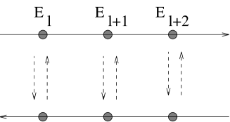
FIG. 1.: Diagram showing coincidence of flux-driven energy levels (corresponding to clockwise and anti-clockwise motion of electrons around ring) at a special flux value (cf. text).

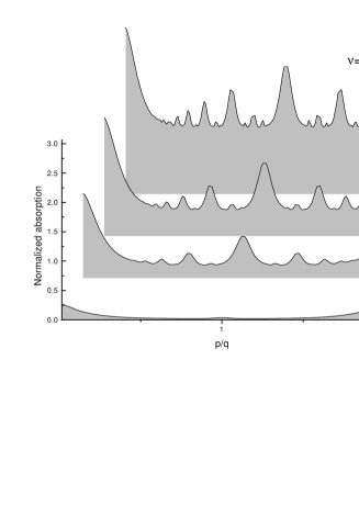
FIG. 2.: The normalized current $J/J_{0}$ as a function of $a=p/q$ for different Landau-Zener tunneling amplitudes, $\tau$. $J_{0}=e\Delta/\hbar$. A of ${\tilde{\nu}}=0.2$ for the dimensionless relaxation rate was used.

REFERENCES

[1] M. Büttiker, Y. Imry, and R. Landauer,
Phys. Rev. A96, 365 (1983).
[2] B. L. Al’tshuler, Pis’ma Zh. Eksp. Teor. Fiz. 41, 530
(1985).
[3] Y. Gefen and D. Thouless, Phys. Rev. Lett. 59, 1752
(1987).
[4] Y. Gefen and D. J. Thouless, Phil. Mag. 56, 1005 (1987).
[5] E. Shimshoni and Y. Gefen, Annals of Physics 210,
16 (1991)
[6] G. Blatter and D. A. Browne, Physical Review B 37, 3856 (1988).
[7] T. Swahn, E. N. Bogachek, Yu. M. Galperin, M. Jonson, and
R. I. Shekhter,
Phys. Rev. Lett. 73, 162 (1994).
[8] L. D. Landau, Phys. Z. Sov. 2,46 (1932); C. Zener,
Proc. Roy. Soc. (London) A 137, 696 (1932).
[9] L. Gorelik, S. Kulinich, Yu. Galperin, M. Jonson and
R. I. Shekhter (unpublished).
[10] See for example J.W.S Cassels ”An Introduction to
Diophantine Approximation.” Cambridge University Press (1957).
[12]
T. Swahn, E. N. Bogachek, Yu. M. Galperin, M. Jonson, and R. I. Shekhter,
Phys. Rev. Lett. 73, 162 (1994).