Effect of screening on shot noise in diffusive mesoscopic conductors

Abstract

Shot noise in diffusive mesoscopic conductors, at finite observation frequencies $\omega$ (comparable to the reciprocal Thouless time $\tau_{T}^{-1}$), is analyzed with an account of screening. At low frequencies, the well-known result $S_{I}(\omega)=2eI/3$ is recovered. This result is valid at arbitrary $\omega\tau_{T}$ for wide conductors longer than the screening length. However, at least for two very different systems, namely, wide and short conductors, and thin conductors over a close ground plane, noise approaches a different fundamental level, $S_{I}(\omega)=eI$, at $\omega\tau_{T}\gg 1$.

The study of non-equilibrium fluctuations of current (”shot noise”) provides important information about microscopic transport properties of conductors. This explains the recent interest in shot noise in various mesoscopic systems (see, e.g., Ref. [2]). In the case of a diffusive mesoscopic conductor ($l\ll L\ll l_{{\rm in}}$, where $L$ is sample’s length, while $l$ and $l_{{\rm in}}$ are the elastic and inelastic scattering lengths, respectively), the low-frequency limit of the shot noise spectral density $S_{I}(\omega)$ was found to be 1/3 of the classical Schottky value $2eI$, where $I$ is the average current through the sample [3, 4, 5].

Most theoretical works on this subject did not discuss screening at all. However, screening, at least in the external electrodes, has to be present in the problem because of the very definition of the noise current (see, e.g., the remarks by Landauer [6]): although the fluctuations leading to the shot noise originate in the conductor itself, the observable noise is that of the current $I^{e}(t)$ induced by these fluctuations in the external circuit. With a permissible simplification, $I^{e}(t)$ can be considered as a current in semi-infinite electrodes, but deep inside them, at distances much larger not only than $l$ and $l_{{\rm in}}$, but also than the screening length from the interface with the conductor.

The purpose of this work was to analyze the frequency dependence of the shot noise in diffusive conductors due to the finite “Thouless” time $\tau_{T}$ of electron diffusion along the sample[7]. We assumed here that the applied voltage is large enough, $eV\gg\hbar/\tau_{T},k_{B}T$ so that in the relevant frequency range $\omega\sim\tau_{T}^{-1}$ we can neglect quantum noise appearing at $\omega\sim eV/\hbar$ [8]. We considered a dirty (metallic or semiconducting) conductor which connects two identical electrodes with screening length $\lambda_{e}$ generally different from that of the conductor ($\lambda)$, within two analytically solvable models. In the first model [Fig. 1(a)] the conductor is assumed to be short and thick ($L\ll t$, where $t$ is the thickness, i.e., the smallest transversal size). In the second case [Fig. 1(b)] we consider a thin conductor located close to a well-conducting ground plane: $t,d\ll L$ (in this case the conductor width $W$ is arbitrary). In both cases we assume that the Fermi level of the conductor is close to that of the electrodes even before they have been brought into contact, so that there are no Schottky barriers at their interfaces (see inset in Fig. 1a). In semiconductor samples, this balance can be readily achieved by either the appropriate doping or electrostatic gating. The interfaces between the electrodes and the conductor are assumed to be smooth (adiabatic) on the scale of the elastic mean free path $l$, but sharper than $\lambda$ and $L$. Thus, the complete hierarchy of length scales assumed in this work is $\lambda_{F}\ll l\ll\Delta x\ll\lambda,\lambda_{e},L\ll l_{{\rm in}},$ where $\lambda_{F}$ is the Fermi surface wavelength in the conductor and $\Delta x$ characterizes the interface smoothness.

Following Nagaev[4], we start with the semiclassical Boltzmann-Langevin equation[9] (justified by the assumption $\lambda_{F}\ll l$). Integration of this equation over the electron momenta leads to a ”drift–diffusion-Langevin” equation for the current density fluctuations

$${\bf j}({\bf r},t)=\sigma({\bf r}){\bf E}({\bf r},t)-D({\bf r}){\bf\nabla}\rho({\bf r},t)+{\bf j}^{s}({\bf r},t),$$ (1)

which is valid even if parameters of the conductor are changing in space (on the scale $\Delta x\gg l$). Here $\rho({\bf r},t)$ and ${\bf E}({\bf r},t)$ are the local fluctuations of charge density and electric field, respectively, and ${\bf j}^{s}({\bf r},t)$ represents the Langevin fluctuation sources of current:

$${\bf j}^{s}({\bf r},t)=e\tau({\bf r})\sum_{{\bf k}}{\bf v}_{{\bf k}}{J}^{s}({\bf r},{\bf k},t),$$ (2)

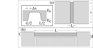
FIG. 1.: Two geometries studied in this work (schematically): (a) - short and wide conductor; (b) - thin and long conductor close to a ground plane. The inset shows the conduction band edge diagram of the structures.

with ${\bf v}_{{\bf k}}$ the velocity of an electron and $\hbar{\bf k}$ its momentum. The correlator for the random sources ${J}^{s}({\bf r},{\bf k},t)$ has been found in [9] (see also [4]). In equations (1) and (2), $\tau({\bf r})$, $\sigma({\bf r})$, and $D({\bf r})$ are the local elastic scattering time, conductivity, and diffusion constant, respectively. Equation (1) should be solved together with the usual Poisson and continuity equations.

For the first model [Fig. 1(a)], we can use 1D versions of all these equations along the dc current direction ($x$), with all the variables integrated over the cross-section $A$ of the conductor. In this case, the combination of the Poisson and continuity equations, integrated over $x$, provides a simple relation between the Fourier images of current and longitudinal electric field:

$$I_{\omega}(x)=\frac{i\omega\varepsilon(x)}{4\pi}E_{\omega}(x)+I_{\omega,}^{e}$$ (3)

where $\varepsilon(x)$ is the local dielectric constant, while $I_{\omega}^{e}$ is an integration constant which has the physical sense of current fluctuations induced deep inside the electrodes (where $E_{\omega}=0$). This constant can be found from the condition that the current fluctuations do not affect the voltage applied to the structure:

$$\delta V_{\omega}=-\int_{-\infty}^{\infty}dx\,E_{\omega}(x)=0.$$ (4)

In our second model [Fig. 1(b)] the electrostatic potential $\Phi_{\omega}(x)$ is completely determined by the local linear density $q_{\omega}(x)$ of electric charge in the conductor:

$$\Phi_{\omega}(x)=q_{\omega}(x)/C_{0},$$ (5)

where $C_{0}$ is the capacitance per unit length. The justification of this equation will be given below.

Combining the 1D equation for current fluctuations with Eq. (3) (first model), or with Eq. (5) and the continuity equation (second model), we get the same simple differential equation

$$\frac{d^{2}I_{\omega}(x)}{dx^{2}}-\kappa^{2}(x,\omega)I_{\omega}(x)=\frac{i\omega}{D^{\prime}(x)}I_{\omega}^{s}(x)-\frac{1}{\Lambda^{2}(x)}I_{\omega}^{e},$$ (6)

where $\kappa(x,\omega)=[\Lambda^{-2}(x)-i\omega/D^{{}^{\prime}}(x)]^{1/2}$ is the effective screening parameter. The effective static screening length $\Lambda$ and diffusion constant $D^{{}^{\prime}}$ are, however, different for our two models. In the first model [Fig. 1(a)], $D^{{}^{\prime}}(x)=D(x)$ and $\Lambda(x)=\lambda(x)$, where $\lambda(x)=\sqrt{\varepsilon(x)D(x)/4\pi\sigma(x)}$ is the usual static screening length.

In the second model, however, the effective parameters are renormalized:

$$D^{{}^{\prime}}(x)=D(x)+\frac{\sigma(x)A}{C_{0}},\,\,\,\,\Lambda(x)=\infty.$$ (7)

The reason for the renormalization of the diffusion constant $D$ is that now the full electro-chemical potential (not only the chemical potential) is proportional to the density $\rho_{\omega}$. The second equation is due to the fact that in this model the electric field created by charge fluctuations is transversal (directed toward the ground plane) and does not lead to accumulation of electrostatic potential along the sample. Equation (6) shows that spatial harmonics with $k\gg|\kappa|=\sqrt{\omega/D^{\prime}}$ contribute negligibly to the current fluctuations $I_{\omega}$. Thus, at frequencies $\omega\sim\tau_{T}^{-1}\ll D^{\prime}/d^{2},D^{\prime}/t^{2}$, we can consider only the wavevectors $k$ (in $x$ direction) which are much smaller than $d^{-1}$, $t^{-1}$. For these harmonics, transversal gradients of all variables dominate, leading immediately to Eq. (5).

In the case of the first model, equation (6) is applicable to both the conductor and the electrodes. The boundary conditions at the interfaces ($x=\pm L/2$) can be derived from the continuity of the current and the electron distribution function at the interfaces. Integrating the latter condition over the electron momenta, and using the continuity equation, we obtain that $I_{\omega}$ and $\lambda^{2}dI_{\omega}/dx$ should be continuous across the interfaces.

Let us consider the most natural case of well-conducting electrodes of macroscopic size ($\gg\lambda_{e},l_{{}_{{\rm in}}}$), with a resistance negligible in comparison with that of the conductor. Scattering in the bulk of such electrodes does not produce considerable current noise (see, e.g., Sec. 4.2 of [2]). The inelastic scattering of nonequilibrium electrons arriving from the conductor also gives negligible noise sources, since the number of scattering events per transferred electron in a dirty conductor is a factor of $(L/l)^{2}\gg 1$ larger than the number of inelastic collisions leading to its thermalization in the electrodes. Therefore, we can neglect the noise sources inside the electrodes, and the solution to Eq. (6) can be presented in the form

$$I_{\omega}(x)=\frac{1}{L}\int_{-\frac{L}{2}}^{\frac{L}{2}}K_{\omega}(x,x^{\prime})I_{\omega}^{s}(x^{\prime})\,dx^{\prime}.$$ (8)

In the case when the conductor and electrodes are uniform along their length (generally, with different $\lambda$), the kernel $K_{\omega}(x,x^{\prime})$ can be expressed with an analytical, though bulky, formula. However, its value at $x=\pm\infty$, giving the current in the external circuit, has a compact form

$$K_{\omega}^{e}(x^{\prime})\equiv K_{\omega}(\pm\infty,x^{\prime})=\frac{1+{\cal A}(\omega)\cosh(\kappa x^{\prime})}{1+{\cal A}(\omega)[\sinh(u)/u]}$$ (9)

where ${\cal A}(\omega)\equiv(k^{2}-1)/[\cosh(u)+(\lambda/\lambda_{e})k\sinh(u)]$, $k\equiv\kappa\lambda$, $u\equiv\kappa L/2$, and $\kappa=\kappa(\omega)$ is the effective screening parameter inside the conductor.

Figures 2(a,b) show the distribution of the charge created by a single, localized, low-frequency current fluctuation source, for the case when the screening in the electrodes is strong, $\lambda_{e}\ll L,\lambda$. One can see that the total charge created by the fluctuation source inside the conductor is compensated by the charge layers of opposite polarity at the conductor-to-electrode interfaces. Equation (9) shows that at low frequencies the external response function is uniform, $K_{0}^{e}(x^{\prime})=1$.

 

FIG. 2.: Charge density induced by a point current source at $x=0.22$ for the cases of strong screening in the electrodes ($L/\lambda_{e}=70$): (a) - low frequency, no internal screening ($L/\Lambda\rightarrow 0$), (b) - low frequency, strong internal screening $(L/\Lambda=30)$, and (c) - high frequency $(|\kappa|L=30)$, no internal static screening. Solid (dotted) lines show the real (imaginary) parts of $\rho_{\omega}$ and $I_{\omega}$. These results are valid for both our models, but in the case of conductor over a ground plane [Fig. 1(b)] there are no charge layers at the interfaces, and $\Lambda$ is always infinite.

In the limit of strong internal screening ($\lambda\ll L$), the local electric dipole formed by the point current fluctuator is screened to a size of the order of $\sim\lambda$, much smaller than the conductor length [Fig. 2(b)]. However, the external current does not vanish and is, moreover, again independent of the fluctuator position. This result stems from the fact that fluctuations of current (rather than charge) do not violate the sample electro-neutrality per se [10], and are not the subject of electrostatic screening at distances of the order of $\lambda.$

Figure 2(c) shows the distribution of the induced charge and current at high frequencies when $|{\rm\kappa}|L\approx(\omega\tau_{T})^{1/2}\gg 1$. Again in the most of the conductor the charge is zero, and the only substantial difference from the case of strong static screening is that the induced current is not constant (which accounts for the finite displacement current).

In the case of our second model shown in Fig. 1(b) the boundary conditions for Eq. (6) generally depend on the exact shape of electrodes. However, in the case of ”perfect” electrodes ($\lambda_{e}\ll\lambda,L$) the boundary conditions are reduced to a simple form

$$\rho_{\omega}=0\,\,\,\,{\rm at}\,\,\,\,x=\pm L/2$$ (10)

(in this limit these boundary conditions are also valid for our first model). Equation (10) together with Eq. (5) make the condition  (4) satisfied automatically, and all the analysis is reduced to the volume of the conductor.

Solution of Eq. (6) with the boundary conditions (10) show that the distribution of charge (but not electric potential!) along the conductor in the second model is generally similar to that in the first model (Fig. 2) in the corresponding limit ($\lambda_{e}\ll L\ll\Lambda$). The only difference is that the conductor over the ground plane does not induce the thin charged layers at the conductor-to-electrode interfaces. The physical reason of this difference is that the charge accumulated in the conductor is now compensated by the equal and opposite charge of the ground plane. Oscillations of this charge are responsible for the fact that at finite frequencies the currents through the interfaces contain not only the ”transport” (symmetric) component $I^{e}$, but also an asymmetric component providing for the re-charging of the sample. As a result the response functions for the left and right interfaces are different:

$$K_{\omega}^{\pm}(x^{\prime})=2u\frac{\cosh(u\pm\kappa x^{\prime})}{\sinh(2u)}.$$ (11)

In order to find the spectral density of the current fluctuations $I^{s}(x,t)$ we need to know the explicit correlation function of the fluctuation sources. In the non-equilibrium limit ($eV/2\gg k_{B}T$) this function can be readily obtained by combining Eq. (2) above with Eqs. (10) and (14) of Ref. [4]:

$$\langle I^{s}(x,t)I^{s}(x^{\prime},0)\rangle=\frac{eIL}{2}\left(1-\frac{4x^{2}}{L^{2}}\right)\delta(x-x^{\prime})\delta(t),$$ (12)

$I$ being the time-averaged current. From Eqs. (8) and (12), the spectral density of fluctuations of the current $I(x,t)$ flowing in an arbitrary cross-section of the conductor is

$$S_{I}(x,\omega) \equiv 2\int_{-\infty}^{\infty}\langle I(x,t)I(x,0)\rangle\exp(i\omega t)dt$$ (13)

$$= \frac{eI}{L}\int_{-\frac{L}{2}}^{\frac{L}{2}}|K_{\omega}(x,x^{\prime})|^{2}\left(1-\frac{4x^{\prime}{}^{2}}{L^{2}}\right)\,dx^{\prime}.$$ (14)

For our first model, the spectral density $S_{I}(\omega)$ of the noise current in electrodes can be found as $S_{I}(\pm\infty,\omega).$ For low frequencies we have $K_{0}^{e}(x^{\prime})=1$, confirming the earlier result $S_{I}(0)=(1/3)\times 2eI$ regardless of the screening properties of the system. At finite frequencies the shot noise depends on the effective screening lengths of the conductor and electrodes. In the high-frequency limit its spectral density is given by

$$S_{I}(\omega)=\frac{eI}{3}\frac{2(\alpha L)^{2}+3}{(\alpha L)^{2}+\beta L+1}\,\,\,\,\,\,{\rm at}\,\,\,\,\,\,\omega\tau_{T}\gg 1,$$ (15)

with $\alpha^{2}\equiv 1/(2\lambda_{e})^{2}+1/(\lambda_{0}\lambda)+2/\lambda_{0}^{2}$, $\beta\equiv 1/\lambda_{e}+2/\lambda_{0}$, and $\lambda_{0}\equiv(2\lambda)^{2}\sqrt{\omega/2D}$. This dependence is shown in Fig. 3(a). In the case of strong screening (either $\lambda\ll L,$ or $\lambda_{e}\ll L,$ or both), the noise suppression factor equals 1/3 even at high frequencies. For intermediate screening ($\lambda\sim L$ or $\lambda_{e}\sim L$) the suppression factor can be as small as 1/5. However, if both effective screening lengths are much larger than $L$, the high frequency noise assumes the value of $(1/2)\times 2eI$, with a crossover near $1/\tau_{T}$ – see Fig. 3(b).

FIG. 3.: (a) - High frequency shot noise in the external circuit as a function of $L/\lambda_{0}$ and $L/\lambda_{e}$. (b) - Frequency dependence of the shot noise, which is valid for short wide conductors at $L\ll\lambda,\lambda_{e}$, and for thin conductors over a ground plane for $L\gg\lambda_{e}$, but arbitrary $\lambda$.

The last result can be interpreted as follows. At high frequencies only the fluctuators near the interface induce noise current in the electrodes (the response functions $K_{\omega}^{e}(x^{\prime})$ exponentially decrease far from the interface), so that each edge of the conductor can be regarded as an independent noise source. Since the electron gas on one side of this ”point contact” is strongly overheated, its noise should obey the classical Schottky formula. The elementary addition of these two independent noise sources with equal effective resistances (see, e.g., Ref. [3]) gives the factor (1/2).

In the ground-plane model, assuming a natural measurement scheme with an instrument symmetric with respect to the ground plane, we accept $I_{\omega}^{e}=[I_{\omega}(-L/2)+I_{\omega}(L/2)]/2$, thus excluding the asymmetric component of the noise current, responsible for re-charging of the conductor. In this case, $S_{I}(\omega)$ is given by the same result as for the first model in the limit $\lambda,\lambda_{e}\gg L$ [Fig. 3(b)] [this can be verified directly by comparing Eq. (11) with Eq. (9)[11]]. Notice, however, that now this limitation is not valid, and a considerable frequency dependence of noise exists for long conductors ($L\gg\lambda_{e},\lambda$).

Despite a considerable recent experimental effort focused on the shot noise in ballistic[12, 13] and diffusive[14, 15, 16] structures, additional experiments are necessary to determine the exact noise suppression factor and its dependence on length and frequency. For wide and short conductors (like in our first model) such measurements can prove to be extremely difficult, since in order to implement low internal screening $(L<\lambda)$ the electron density has to be very low and the sample very short. However, it seems that the frequency dependence predicted here could be observed in systems close to our ground-plane model [Fig. 1(b)], for example in inversion layers of field-effect transistors and other 2DEG structures. With typical values of $D^{\prime}\simeq D\sim 10^{3}\,{\rm cm}^{2}/{\rm s}$ and $L\sim 10\mu{\rm m}$[14], the expected crossover frequency is of the order of 5 GHz, i.e., within the range currently available for accurate noise measurements (cf. Refs. [12, 16]).

To summarize, we have shown that effects of screening have to be taken into account in order to obtain realistic results for shot noise in mesoscopic conductors at finite frequencies ($\omega\tau_{T}\geq 1$). For relatively short conductors ($L\ll\lambda,\lambda_{e}$), or for long, thin conductors close to a ground plane, noise should approach a level of $(1/2)\times 2eI$ at high frequencies.

We are grateful to M. Büttiker for numerous discussions and for bringing to our attention an error in the initial version of the manuscript. We are also grateful to K. E. Nagaev and R. J. Schoelkopf for making their results available prior to publication, to S. K. Tolpygo for discussions, and to the anonymous referee for a valuable comment concerning the experimental observation of the predicted effects. The work was supported in part by DOE’s Grant #DE-FG02-95ER14575. We thank the Institute for Nuclear Theory at the University of Washington for its hospitality and the DOE for partial support during the completion of this work.

REFERENCES

- [1] Electronic address: yehuda@hana.physics.sunysb.edu
- [2] For a recent review, see M. J. M. de Jong and C. W. J. Beenakker, cond-mat/9611140 (1996). See also Sh. Kogan, Electronic noise and fluctuation in solids (Cambridge, Cambridge, 1996).
- [3] C. W. J. Beenakker and M. Büttiker, Phys. Rev. B 46, 1889 (1992).
- [4] K. E. Nagaev, Phys. Lett. A 169, 103 (1992).
- [5] Yu. Nazarov, Phys. Rev. Lett. 73, 134 (1994).
- [6] R. Landauer, Physica B 227, 156 (1996).
- [7] In contrast with extensive studies of high-frequency noise in other mesoscopic structures [for a review, see, e.g., M. Büttiker, J. Math. Phys. 37, 4793 (1996)], in diffusive conductors this problem was analyzed only in Ref. [8].
- [8] B. L. Altshuler, L. S. Levitov, and A. Yu. Yakovets, Pis’ma Zh. Eksp. Teor. Fiz. 59, 821 (1994) [JETP Lett. 59, 857 (1994)]. In that work only the case has been considered, so that the crossover at predicted in the present work could not be traced.
- [9] Sh. M. Kogan and A. Ya. Shul’man, Zh. Eksp. Teor. Fiz. 56, 862 (1969) [Sov. Phys. JETP 29, 467 (1969)].
- [10] See, e.g., D. Pines and P. Nozieres, The Theory of Quantum Liquids (Benjamin, New York, 1966), Sec. 3.5.
- [11] Notice that the high-frequency noise at the conductor-electrode interfaces is , in agreement with K.E. Nagaev, cond-mat/9706024.
- [12] M. Reznikov, M. Heiblum, H. Shtrikman, and D. Mahalu, Phys. Rev. Lett. 75, 3340 (1995).
- [13] A. Kumar, L. Saminadayar, D. C. Glattli, Y. Jin, and B. Etienne, Phys. Rev. Lett. 76, 2778 (1996).
- [14] F. Liefrink, J. I. Dijkhuis, M. J. M. de Jong, L. W. Molenkamp, and H. van Houten Phys. Rev. B 49, 14066 (1994).
- [15] A.H. Steinbach, J.M. Martinis, and M.H. Devoret, Phys. Rev. Lett. 76, 3806 (1996).
- [16] R. J. Schoelkopf, P. J. Burke, A. Kozhevnikov, D. E. Prober, and M. J. Rooks, Phys. Rev. Lett. 78, 3370 (1997).