Single particle excitations of the Kondo lattice

Abstract

We present a simple theory for the description of the single particle excitations of the Kondo lattice model. We derive an ‘effective Hamiltonian’ which describes the coherent propagation of single particle-like fluctuations on a strong coupling groundstate. Even for $f$-electrons which are replaced by Kondo-spins, the resulting spectral function obeys the Luttinger theorem including the $f$-electrons, and our calculation reproduces the complicated evolution of the spectral function with electron density seen in numerical studies.

The theoretical description of the Kondo lattice remains an unsolved problem of solid state physics, yet the solution of this problem is crucial for understanding the anomalous prperties of $f$-electron metals[1]. The simplest model which incorporates the essential physics is the Kondo lattice model

$$H = \sum_{\mathchoice{{\hbox{\boldmath$\displaystyle k$}}}{{\hbox{\boldmath$\textstyle k$}}}{{\hbox{\boldmath$\scriptstyle k$}}}{{\hbox{\boldmath$\scriptscriptstyle k$}}},\sigma}\epsilon(\mathchoice{{\hbox{\boldmath$\displaystyle k$}}}{{\hbox{\boldmath$\textstyle k$}}}{{\hbox{\boldmath$\scriptstyle k$}}}{{\hbox{\boldmath$\scriptscriptstyle k$}}})c_{\mathchoice{{\hbox{\boldmath$\displaystyle k$}}}{{\hbox{\boldmath$\textstyle k$}}}{{\hbox{\boldmath$\scriptstyle k$}}}{{\hbox{\boldmath$\scriptscriptstyle k$}}},\sigma}^{\dagger}c_{\mathchoice{{\hbox{\boldmath$\displaystyle k$}}}{{\hbox{\boldmath$\textstyle k$}}}{{\hbox{\boldmath$\scriptstyle k$}}}{{\hbox{\boldmath$\scriptscriptstyle k$}}},\sigma}-V\sum_{i,\sigma}(c_{i,\sigma}^{\dagger}f_{i,\sigma}+H.c.)$$ (1)

$$- \epsilon_{f}\sum_{i,\sigma}n_{i,\sigma}+U\sum_{i}n_{i,\uparrow}n_{i,\downarrow}.$$ (2)

Here we consider the ‘minimal’ model, where each unit cell contains two orbitals, one of them for the uncorrelated conduction electrons the other for the strongly correlated $f$-electrons. Then, $c_{i,\sigma}^{\dagger}$ ($f_{i,\sigma}^{\dagger}$) creates a conduction electron ($f$-electron) in cell $i$, $n_{i,\sigma}$$=$$f_{i,\sigma}^{\dagger}f_{i,\sigma}$, and $\epsilon(\mathchoice{{\hbox{\boldmath$\displaystyle k$}}}{{\hbox{\boldmath$\textstyle k$}}}{{\hbox{\boldmath$\scriptstyle k$}}}{{\hbox{\boldmath$\scriptscriptstyle k$}}})$$=$$\sum_{i,j}exp(i\mathchoice{{\hbox{\boldmath$\displaystyle k$}}}{{\hbox{\boldmath$\textstyle k$}}}{{\hbox{\boldmath$\scriptstyle k$}}}{{\hbox{\boldmath$\scriptscriptstyle k$}}}\cdot(\mathchoice{{\hbox{\boldmath$\displaystyle R$}}}{{\hbox{\boldmath$\textstyle R$}}}{{\hbox{\boldmath$\scriptstyle R$}}}{{\hbox{\boldmath$\scriptscriptstyle R$}}}_{i}-\mathchoice{{\hbox{\boldmath$\displaystyle R$}}}{{\hbox{\boldmath$\textstyle R$}}}{{\hbox{\boldmath$\scriptstyle R$}}}{{\hbox{\boldmath$\scriptscriptstyle R$}}}_{j}))\;t_{i,j}$ is the Fourier transform of the inter-cell hopping integral $t_{i,j}$ for $c$ electrons. For simplicity we consider only the symmetric case, $U=2\epsilon_{f}$. For $U$$\gg$$V$ (2) can be reduced to

$$H_{sc}=\sum_{\mathchoice{{\hbox{\boldmath$\displaystyle k$}}}{{\hbox{\boldmath$\textstyle k$}}}{{\hbox{\boldmath$\scriptstyle k$}}}{{\hbox{\boldmath$\scriptscriptstyle k$}}},\sigma}\epsilon(\mathchoice{{\hbox{\boldmath$\displaystyle k$}}}{{\hbox{\boldmath$\textstyle k$}}}{{\hbox{\boldmath$\scriptstyle k$}}}{{\hbox{\boldmath$\scriptscriptstyle k$}}})c_{\mathchoice{{\hbox{\boldmath$\displaystyle k$}}}{{\hbox{\boldmath$\textstyle k$}}}{{\hbox{\boldmath$\scriptstyle k$}}}{{\hbox{\boldmath$\scriptscriptstyle k$}}},\sigma}^{\dagger}c_{\mathchoice{{\hbox{\boldmath$\displaystyle k$}}}{{\hbox{\boldmath$\textstyle k$}}}{{\hbox{\boldmath$\scriptstyle k$}}}{{\hbox{\boldmath$\scriptscriptstyle k$}}},\sigma}+J\sum_{i}\mathchoice{{\hbox{\boldmath$\displaystyle S$}}}{{\hbox{\boldmath$\textstyle S$}}}{{\hbox{\boldmath$\scriptstyle S$}}}{{\hbox{\boldmath$\scriptscriptstyle S$}}}_{i,c}\cdot\mathchoice{{\hbox{\boldmath$\displaystyle S$}}}{{\hbox{\boldmath$\textstyle S$}}}{{\hbox{\boldmath$\scriptstyle S$}}}{{\hbox{\boldmath$\scriptscriptstyle S$}}}_{i,f}$$ (3)

where $\mathchoice{{\hbox{\boldmath$\displaystyle S$}}}{{\hbox{\boldmath$\textstyle S$}}}{{\hbox{\boldmath$\scriptstyle S$}}}{{\hbox{\boldmath$\scriptscriptstyle S$}}}_{i,c}$ $(\mathchoice{{\hbox{\boldmath$\displaystyle S$}}}{{\hbox{\boldmath$\textstyle S$}}}{{\hbox{\boldmath$\scriptstyle S$}}}{{\hbox{\boldmath$\scriptscriptstyle S$}}}_{i,f})$ denotes the spin operator for conduction electrons ($f$-electrons) in cell $i$ and $J=4V^{2}/\epsilon_{f}$. One problem which by many is believed to be at the heart of the solution is the way in which the more or less localized $f$-electrons, which are replaced by mere spin degrees of freedom in the strong coupling version (3) , participate in the formation of the Fermi surface. De Haas-van Alphen experiments on heavy Fermion metals[2] as well as computer simulations of Kondo lattice models[3, 4] suggest that despite their ‘frozen’ charge degrees of freedom the $f$-electrons participate in the Fermi surface volume as if they were uncorrelated. The limiting cases $V$$=$$0$, $J$$=$$0$, which obviously do not allow for participation of the $f$ electrons in the Fermi surface, therefore represent singular points, so that a perturbation expansion in the (small) parameters $V$ or $J$ may not be expected to give meaningful results. Rather, the interaction between $f$-spins and conduction electrons must be incorporated in a non-perturbative way, in a similar manner as the single-impurity Kondo effect[5]. It is the purpose of the present manuscript to present a minimum effort theory for the Kondo lattice which is based on this requirement and shows how the nominal participation of the localized electrons in the Fermi surface can be understood even in the complete absence of true hybridization. We describe the system by an ‘effective Hamiltonian’ for the Fermion-like charge fluctuations on top of a strong coupling ground state, and show that this treatment leads to remarkable agreement with the scenario inferred from numerical simulations.
As a starting point, we take the case of half-filling (i.e. two electrons/unit cell, corresponding to the ‘Kondo insulator’) and vanishing inter-cell hopping integrals $t_{i,j}$. In this limit, the lattice ground state is simply the product of $N$ single-cell ground states, each of them being

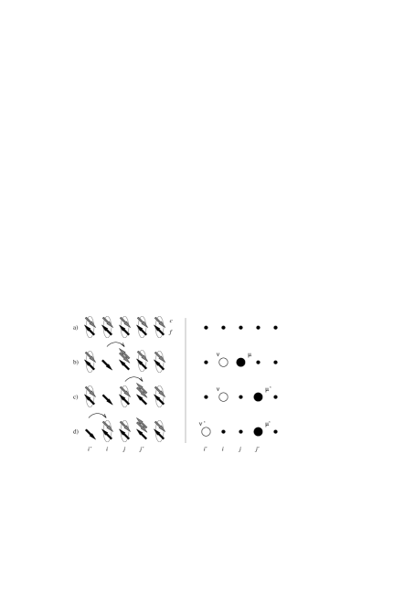
FIG. 1.: Charge fluctuations and their propagation (left panel) and their representation in terms of ‘model Fermions’ (right panel).

a two-electron singlet state (see the state (a) in Figure 1). In the following we consider this product state as a kind of ‘vaccuum’. This state clearly is a total singlet, and has no magnetic order; it thus is appropriate to discuss the paramagnetic phase of primary interest. Switching on the $t_{i,j}$ then produces ‘charge fluctuations’ on this vacuum: an electron can jump from a cell $i$ to another cell $j$, leaving the cell $i$ in a single electron eigenstate with number $\nu$, and the cell $j$ in a three electron eigenstate with number $\mu$ (see state (b) in Figure 1). We note that the Hamiltonian (2) allows for two such eigen states of a single cell, the strong coupling version (3) only for one. In further steps, these charge fluctuations can propagate: an electron from the three-fold occupied cell $j$ can hop to another neighbor $j^{\prime}$ leaving cell $j$ with two electrons and $j^{\prime}$ in a three electron state (see Figure 1c ) or, alternatively, an electron can jump from another neighbor $i^{\prime}$ into cell $i$, leaving $i$ in a two electron state, $i^{\prime}$ in a single electron state. When there is only one $c$ orbital/unit cell, the single cell states of both $1$ or $3$ electrons are spin dublets, i.e. these states have the spin quantum numbers of ordinary electrons. As our basic approximation we now restrict the Hilbert space such that whenever there are $2$ electrons in one cell, they are in the singlet ground state. This restriction implies that the propagating charge fluctuations do not ‘leave a trace’ of excited cells, i.e. their motion under this constraint becomes completely coherent. We can then interpret the first step in Figure 1 as a pair creation process, where two ‘book keeping Fermions’ are created on nearest neighbors in the vacuum state, and the subsequent steps in Figure 1 as a propagation of these Fermions. More precisely, if cell number $i$ is in the $\nu^{th}$ single electron eigenstate with $z$-spin $\sigma$ we interpret this as presence of a hole-like Fermion, created by $a_{\nu,\sigma}^{\dagger}$, whereas the cell being in the $\mu^{th}$ three electron eigenstate with $z$-spin $\sigma$ is modelled by the presence of an electron-like Fermion, created by $b_{\mu,\sigma}^{\dagger}$. Within our restricted Hilbert space the dynamics of the model then is decribed by the Hamiltonian $H_{eff}$$=$${\cal P}H{\cal P}$ where

$$H=\sum_{i,\sigma}(\;\Delta\;a_{i,\sigma}^{\dagger}a_{i,\sigma}+\bar{\Delta}\;b_{i,\sigma}^{\dagger}b_{i,\sigma}\;)+\sum_{i,j,\sigma}[\;(\;V_{i,j}\;b_{j,\sigma}^{\dagger}a_{i,\bar{\sigma}}^{\dagger}$$ (4)

$$+V^{\prime}_{i,j}\;a_{j,\sigma}^{\dagger}a_{i,\sigma}+V^{\prime\prime}_{i,j,}\;b_{j,\sigma}^{\dagger}b_{i,\sigma}\;)+H.c.\;].$$ (5)

and ${\cal P}$ projects onto the subspace of states where no site is occupied by more than one Fermion. This kinematic constraint reflects the fact that the state of a given cell must be unique. (for the sake of brevity we have suppressed the state indices $\mu,\nu$ in (5)). The procedere is very much analogous to spin wave theory, with the sole difference that we are considering Fermionic charge fluctuations rather than Bosonic spin fluctuations. Due to the product nature of the basis states, the various matrix elements $V$, $V^{\prime}$ and $V^{\prime\prime}$ in (5) are easily expressed in terms of the electron removal and addition matrix elements of a single cell, $m_{PES,\nu}=\langle\Psi_{\nu}^{(1)}|c_{\sigma}|\Psi_{0}^{(2)}\rangle$ and $m_{IPES,\mu}=\langle\Psi_{\mu}^{(3)}|c_{\sigma}^{\dagger}|\Psi_{0}^{(2)}\rangle$. For example $V_{(i,\nu),(j,\mu)}$$=$$t_{i,j}\;m_{PES,\nu}\;m_{IPES,\mu}$ (here $|\Psi_{\mu}^{(n)}\rangle$ denotes the $\mu^{th}$ eigenstate of a cell with $n$ electrons). The ‘on site energies’ are defined as $\Delta_{\nu}$$=$$E_{\nu}-E_{0}$.
In analogy with linear spin wave theory we now relax the constraint enforced by ${\cal P}$, whereupon the Hamiltonian (5) is readily solved by Bogoliubov transformation, $\gamma_{\mathchoice{{\hbox{\boldmath$\displaystyle k$}}}{{\hbox{\boldmath$\textstyle k$}}}{{\hbox{\boldmath$\scriptstyle k$}}}{{\hbox{\boldmath$\scriptscriptstyle k$}}},\lambda,\sigma}^{\dagger}$$=$$\sum_{\nu}u_{\mathchoice{{\hbox{\boldmath$\displaystyle k$}}}{{\hbox{\boldmath$\textstyle k$}}}{{\hbox{\boldmath$\scriptstyle k$}}}{{\hbox{\boldmath$\scriptscriptstyle k$}}},\lambda,\sigma}^{(\nu)}a_{\nu,-\mathchoice{{\hbox{\boldmath$\displaystyle k$}}}{{\hbox{\boldmath$\textstyle k$}}}{{\hbox{\boldmath$\scriptstyle k$}}}{{\hbox{\boldmath$\scriptscriptstyle k$}}},\bar{\sigma}}+\sum_{\mu}u_{\mathchoice{{\hbox{\boldmath$\displaystyle k$}}}{{\hbox{\boldmath$\textstyle k$}}}{{\hbox{\boldmath$\scriptstyle k$}}}{{\hbox{\boldmath$\scriptscriptstyle k$}}},\lambda,\sigma}^{(\mu)}b_{\mu,\mathchoice{{\hbox{\boldmath$\displaystyle k$}}}{{\hbox{\boldmath$\textstyle k$}}}{{\hbox{\boldmath$\scriptstyle k$}}}{{\hbox{\boldmath$\scriptscriptstyle k$}}},\sigma}^{\dagger}$. A possibility to treat the constraint in a more rigorous fashion would be to apply complete Gutzwiller projection to the wave functions obtained from (5); anticipating that the main effect is a renormalization of the matrix elements, we may expect that a calculation without the constraint at least qualitatively reproduces the correct one. Our main justification for this approximation, however, is the good agreement with exact cluster results as discussed below. As mentioned above, the Hamiltonian (5) may be thought of as describing the coherent propagation of single particle-like fluctuations ‘on top of’ the strong coupling ‘vacuum’ state. One may expect that there will also be e.g. spin-like fluctuations, which would correspond to a cell being occupied by two electrons in a triplet state. The creation of these spin excitations by the propagating charge fluctuations would be described by terms of the form $\;a_{i,\tau}^{\dagger}\vec{S}_{j,}^{\dagger}\cdot\vec{\sigma}_{\tau,\tau^{\prime}}a_{j,\tau^{\prime}}$, where $\vec{S}_{j}^{\dagger}$ is a bosonic spin-triplet operator. Such terms could be treated e.g. within the ‘rainbow diagram’ approximation[7], but in the present manuscript we restrict ourselves to the coherent motion.
For the strong coupling limit (3) the calculation becomes particularly simple: one finds $m_{PES}$$=$$m_{IPES}$$=1/\sqrt{2}$ whence $V_{i,j}$$=$$-V^{\prime}_{i,j}$$=$$V^{\prime\prime}_{i,j}$$=$$t_{i,j}/2$, $\Delta$$=$$\bar{\Delta}$$=$$3J/4$, so that the dispersion relation reads

$$E_{\pm}(\mathchoice{{\hbox{\boldmath$\displaystyle k$}}}{{\hbox{\boldmath$\textstyle k$}}}{{\hbox{\boldmath$\scriptstyle k$}}}{{\hbox{\boldmath$\scriptscriptstyle k$}}})=(1/2)\;[\;\epsilon(\mathchoice{{\hbox{\boldmath$\displaystyle k$}}}{{\hbox{\boldmath$\textstyle k$}}}{{\hbox{\boldmath$\scriptstyle k$}}}{{\hbox{\boldmath$\scriptscriptstyle k$}}})\pm\sqrt{\Delta^{2}+\epsilon(\mathchoice{{\hbox{\boldmath$\displaystyle k$}}}{{\hbox{\boldmath$\textstyle k$}}}{{\hbox{\boldmath$\scriptstyle k$}}}{{\hbox{\boldmath$\scriptscriptstyle k$}}})^{2}}\;].$$ (6)

Formally, this is equivalent to the hybridization of a dispersionless ‘effective’ $f$-level in the band center with a free electron band with dispersion $\epsilon(\mathchoice{{\hbox{\boldmath$\displaystyle k$}}}{{\hbox{\boldmath$\textstyle k$}}}{{\hbox{\boldmath$\scriptstyle k$}}}{{\hbox{\boldmath$\scriptscriptstyle k$}}})$, the strength of the ‘nominal’ mixing element being $3J/4$. It should be noted, however, that the resulting energy gap of $\Delta$ does not arise from the formation of a bonding and antibonding combination of $c$-like and $f$-like Bloch states, as in the hybridization model; rather, this gap originates from the energy cost to break two intra-cell singlets in the course of a charge fluctuation. This gap therefore is of a similar nature as the energy gap in a superconductor.
Having computed the eigenvalue spectrum, we proceed to the computation of the single particle spectral function. This requires to resolve the ‘ordinary’ electron operators in terms of the model Fermions. Taking into account our basic assumption, namely that a single cell with $2$ electrons can only be in its ground state, we can expand e.g. the electron annihilation operator as

$$c_{i,\sigma}=\sum_{\nu}m_{PES,\nu}a_{i,\nu,\bar{\sigma}}^{\dagger}+\sum_{\mu}m_{IPES,\mu}^{*}b_{i,\mu,\sigma}.$$ (7)

Then, Figure 2a shows the single particle spectral function for a $1D$ chain of the full Kondo lattice (2) at half-filling (see e.g. Ref.[3] for a precise definition of this quantity). Particle-hole symmetry implies that the Fermi energy is zero in this case. It is obvious at first sight, that our calculation is in excellent agreement with the results of exact diagonalization[3]. To begin with, unlike any band theory approach, our calculation gives the correct number of ‘bands’: the nearly dispersionless upper and lower Hubbard bands with almost pure $f$ character, and the two ‘hybridization bands’ which resemble the result for the strong coupling limit, (6). The hybridization bands change their character from high intensity $c$-like to weak intensity $f$-like near $\pi/2$, i.e. the Fermi momentum of the unhybridized $d$ electrons. Note that while the dispersion of these bands could be modelled by band theory, the sharp drop of spectral weight at $\pi/2$ could not. In the Kondo limit, where the strength of the ‘ effective hybridization’ is small, there are extended regions of flat

FIG. 2.: Single particle spectral function for the $1D$ Kondo lattice with $\epsilon(k)$$=$$-2\cos(k)$, $U$$=$$10$ and $V$$=0.5$. The electron density is $2.0$/unit cell in (a) (i.e. half-filling) and $1.6$/unit cell in (b). Full lines (dashed lines) correspond to $f$-like ($c$-like) spectral weight. Peaks to the right (left) of the vertical line correspond to electron creation (annihilation).

(i.e. ‘heavy’) bands. Quite obviously the basic idea of our approach, namely to broaden the ionization and affinity states of a single cell into bands works well as far as the dispersion of energy and spectral weight is concerned. The present approximation does not incorporate the infrared divergences which occur in the impurity problem, and therefore does not reproduce the parameter dependences of the low energy scales[6]. For example the lowering of the total energy/site as compared to the noninteracting case is $\sim\Delta^{2}ln(W/\Delta)$ when calculated from (6), and the $f$-like spectral weight $Z_{f}$ of the ‘heavy bands’ has the same functional dependence on the parameter values as in the single cell problem, i.e. $Z$$\sim$$(V/\epsilon_{f})^{2}$.
We proceed to the doped case and first consider the expression for the electron number operator. We give explicit expressions only for the strong coupling limit (3), but all considerations for the full Kondo lattice are completely analogous. In the ‘vacuum state’, the number of electrons is $2N$ and the presence of an $a$-Fermion ($b$-Fermion) decreases (increases) the electron number by $1$, so that the electron number operator should be simply

$$N_{e}=\sum_{\mathchoice{{\hbox{\boldmath$\displaystyle k$}}}{{\hbox{\boldmath$\textstyle k$}}}{{\hbox{\boldmath$\scriptstyle k$}}}{{\hbox{\boldmath$\scriptscriptstyle k$}}},\sigma}(\;a_{\mathchoice{{\hbox{\boldmath$\displaystyle k$}}}{{\hbox{\boldmath$\textstyle k$}}}{{\hbox{\boldmath$\scriptstyle k$}}}{{\hbox{\boldmath$\scriptscriptstyle k$}}},\sigma}a_{\mathchoice{{\hbox{\boldmath$\displaystyle k$}}}{{\hbox{\boldmath$\textstyle k$}}}{{\hbox{\boldmath$\scriptstyle k$}}}{{\hbox{\boldmath$\scriptscriptstyle k$}}},\sigma}^{\dagger}+b_{\mathchoice{{\hbox{\boldmath$\displaystyle k$}}}{{\hbox{\boldmath$\textstyle k$}}}{{\hbox{\boldmath$\scriptstyle k$}}}{{\hbox{\boldmath$\scriptscriptstyle k$}}},\sigma}^{\dagger}b_{\mathchoice{{\hbox{\boldmath$\displaystyle k$}}}{{\hbox{\boldmath$\textstyle k$}}}{{\hbox{\boldmath$\scriptstyle k$}}}{{\hbox{\boldmath$\scriptscriptstyle k$}}},\sigma}\;)=\sum_{\mathchoice{{\hbox{\boldmath$\displaystyle k$}}}{{\hbox{\boldmath$\textstyle k$}}}{{\hbox{\boldmath$\scriptstyle k$}}}{{\hbox{\boldmath$\scriptscriptstyle k$}}},\mu,\sigma}\gamma_{\mathchoice{{\hbox{\boldmath$\displaystyle k$}}}{{\hbox{\boldmath$\textstyle k$}}}{{\hbox{\boldmath$\scriptstyle k$}}}{{\hbox{\boldmath$\scriptscriptstyle k$}}},\mu,\sigma}^{\dagger}\gamma_{\mathchoice{{\hbox{\boldmath$\displaystyle k$}}}{{\hbox{\boldmath$\textstyle k$}}}{{\hbox{\boldmath$\scriptstyle k$}}}{{\hbox{\boldmath$\scriptscriptstyle k$}}},\mu,\sigma}.$$ (8)

This operator counts both localized and conduction electrons, so that reducing the electron density $\rho_{e}$ below $2$ will give a Fermi edge in the lower hybridization band which satisfies a ‘nominal’ Luttinger theorem, i.e. including the $f$ -electrons. The physical origin, however, is the fact that we have a density $2-\rho_{e}$ of holes in the insulating ‘singlet background’. This results in a ‘hole pocket’ of volume $(1-\rho_{e}/2)$, which however is nominally equivalent to a Luttinger Fermi surface including the $f$-electrons. There is, however, an extra complication: the electron number should also equal the integrated PES weight, which is given by the expectation value of

$$N_{e}^{\prime}=N+\sum_{\mathchoice{{\hbox{\boldmath$\displaystyle k$}}}{{\hbox{\boldmath$\textstyle k$}}}{{\hbox{\boldmath$\scriptstyle k$}}}{{\hbox{\boldmath$\scriptscriptstyle k$}}},\sigma}c_{\mathchoice{{\hbox{\boldmath$\displaystyle k$}}}{{\hbox{\boldmath$\textstyle k$}}}{{\hbox{\boldmath$\scriptstyle k$}}}{{\hbox{\boldmath$\scriptscriptstyle k$}}},\sigma}^{\dagger}c_{\mathchoice{{\hbox{\boldmath$\displaystyle k$}}}{{\hbox{\boldmath$\textstyle k$}}}{{\hbox{\boldmath$\scriptstyle k$}}}{{\hbox{\boldmath$\scriptscriptstyle k$}}},\sigma}.$$ (9)

The first term on the r.h.s. is the contribution of the $f$-electrons’ lower Hubbard band. Using (7), which now reads $c_{\mathchoice{{\hbox{\boldmath$\displaystyle k$}}}{{\hbox{\boldmath$\textstyle k$}}}{{\hbox{\boldmath$\scriptstyle k$}}}{{\hbox{\boldmath$\scriptscriptstyle k$}}},\sigma}$$=$$(1/\sqrt{2})(a_{\mathchoice{{\hbox{\boldmath$\displaystyle k$}}}{{\hbox{\boldmath$\textstyle k$}}}{{\hbox{\boldmath$\scriptstyle k$}}}{{\hbox{\boldmath$\scriptscriptstyle k$}}},\sigma}^{\dagger}+b_{\mathchoice{{\hbox{\boldmath$\displaystyle k$}}}{{\hbox{\boldmath$\textstyle k$}}}{{\hbox{\boldmath$\scriptstyle k$}}}{{\hbox{\boldmath$\scriptscriptstyle k$}}},\sigma})$, this becomes

$\displaystyle N+\frac{1}{2}\sum_{\mathchoice{{\hbox{\boldmath$\displaystyle k$}}}{{\hbox{\boldmath$\textstyle k$}}}{{\hbox{\boldmath$\scriptstyle k$}}}{{\hbox{\boldmath$\scriptscriptstyle k$}}},\sigma}(a_{\mathchoice{{\hbox{\boldmath$\displaystyle k$}}}{{\hbox{\boldmath$\textstyle k$}}}{{\hbox{\boldmath$\scriptstyle k$}}}{{\hbox{\boldmath$\scriptscriptstyle k$}}},\sigma}a_{\mathchoice{{\hbox{\boldmath$\displaystyle k$}}}{{\hbox{\boldmath$\textstyle k$}}}{{\hbox{\boldmath$\scriptstyle k$}}}{{\hbox{\boldmath$\scriptscriptstyle k$}}},\sigma}^{\dagger}+b_{\mathchoice{{\hbox{\boldmath$\displaystyle k$}}}{{\hbox{\boldmath$\textstyle k$}}}{{\hbox{\boldmath$\scriptstyle k$}}}{{\hbox{\boldmath$\scriptscriptstyle k$}}},\sigma}^{\dagger}b_{\mathchoice{{\hbox{\boldmath$\displaystyle k$}}}{{\hbox{\boldmath$\textstyle k$}}}{{\hbox{\boldmath$\scriptstyle k$}}}{{\hbox{\boldmath$\scriptscriptstyle k$}}},\sigma}+a_{\mathchoice{{\hbox{\boldmath$\displaystyle k$}}}{{\hbox{\boldmath$\textstyle k$}}}{{\hbox{\boldmath$\scriptstyle k$}}}{{\hbox{\boldmath$\scriptscriptstyle k$}}},\sigma}^{\dagger}b_{\mathchoice{{\hbox{\boldmath$\displaystyle k$}}}{{\hbox{\boldmath$\textstyle k$}}}{{\hbox{\boldmath$\scriptstyle k$}}}{{\hbox{\boldmath$\scriptscriptstyle k$}}},\sigma}^{\dagger}+b_{\mathchoice{{\hbox{\boldmath$\displaystyle k$}}}{{\hbox{\boldmath$\textstyle k$}}}{{\hbox{\boldmath$\scriptstyle k$}}}{{\hbox{\boldmath$\scriptscriptstyle k$}}},\sigma}a_{\mathchoice{{\hbox{\boldmath$\displaystyle k$}}}{{\hbox{\boldmath$\textstyle k$}}}{{\hbox{\boldmath$\scriptstyle k$}}}{{\hbox{\boldmath$\scriptscriptstyle k$}}},\sigma}).$

Counting the electrons in real space on one hand and integrating the spectral weight on the other hand thus results in different expressions for the electron number. This can hardly be a surprise, since in a strongly correlated electron system spectral weight and band structure are decoupled to a large extent. As an example let us consider the extreme Kondo limit, and assume that we are gradually reducing the electron density from the ‘Kondo insulator value’ of $2$. The chemical potential corresponding to the real-space electron count (8) then will cut more and more into the ‘heavy’ band, to produce the nominal Luttinger Fermi surface volume. Since the spectral weight per $\textstyle k$-point is much smaller than $1$ for the ‘heavy’ band, however, the amount of spectral weight which crosses from PES to IPES as the the Fermi momentum changes can never be consistent with the electron number. A simple rigid band picture therefore must fail to maintain the consistency of electron number and integrated spectral weight. To cope with this problem, we choose the simplest possible solution and enforce the consistency of ‘ordinary’ electron count and spectral weight integration by adding both expressions, (8) and (9), for the electron number to the Hamiltonian, each of them multiplied by a separate Lagrange multiplier: $H\rightarrow H+\mu N_{e}+\lambda N_{e}^{\prime}$. The notion of ‘two chemical potentials’ may seem awkward at first sight, but as we will show now, this approach results in a remarkable consistency with the numerical results. For the strong coupling limit (3) this substitution gives the same dispersion relation as (6), however with the replacements $E(\mathchoice{{\hbox{\boldmath$\displaystyle k$}}}{{\hbox{\boldmath$\textstyle k$}}}{{\hbox{\boldmath$\scriptstyle k$}}}{{\hbox{\boldmath$\scriptscriptstyle k$}}})$$\rightarrow$$E(\mathchoice{{\hbox{\boldmath$\displaystyle k$}}}{{\hbox{\boldmath$\textstyle k$}}}{{\hbox{\boldmath$\scriptstyle k$}}}{{\hbox{\boldmath$\scriptscriptstyle k$}}})$$-$$\mu$ and $\epsilon(\mathchoice{{\hbox{\boldmath$\displaystyle k$}}}{{\hbox{\boldmath$\textstyle k$}}}{{\hbox{\boldmath$\scriptstyle k$}}}{{\hbox{\boldmath$\scriptscriptstyle k$}}})$$\rightarrow$$\epsilon(\mathchoice{{\hbox{\boldmath$\displaystyle k$}}}{{\hbox{\boldmath$\textstyle k$}}}{{\hbox{\boldmath$\scriptstyle k$}}}{{\hbox{\boldmath$\scriptscriptstyle k$}}})$$-$$\lambda$. The effect of these modifications can be seen in Figure 2b, which shows the spectral function for the Kondo lattice away from half-filling. To begin with, the $f$-like upper and lower hubbard band remain unaffected by the change in electron concentration. The Lagrange multiplier $\mu$ acts like a standard chemical potential, which cuts into the ‘heavy’ band and, as discussed above, produces a Fermi

FIG. 3.: Momentum distribution for the strong coupling limit for different values of $J$, $\rho_{c}=0.5$.

surface consistent with the nominal Luttinger theorem. On the other hand, the Lagrange multiplier for the spectral weight, $\lambda$, modifies the dispersion relation far from the true Fermi momentum: the occupied part of the $c$-like band structure shortens, the unoccupied part grows. In fact, the change of the $c$-like spectral weight alone is very reminiscent of what is expected for free (i.e. unhybridized) conduction electrons. This can be understood by carrying on the formal analogy of (6) with a hybridization gap picture: $\lambda$ obviously plays the role of the ‘on-site energy’ of the effective $f$ level. Next, in the Kondo limit $J\ll t$ the momentum distribution for the conduction electrons, $n_{c}(\mathchoice{{\hbox{\boldmath$\displaystyle k$}}}{{\hbox{\boldmath$\textstyle k$}}}{{\hbox{\boldmath$\scriptstyle k$}}}{{\hbox{\boldmath$\scriptscriptstyle k$}}})$ has the limiting behaviour $n_{c}(\mathchoice{{\hbox{\boldmath$\displaystyle k$}}}{{\hbox{\boldmath$\textstyle k$}}}{{\hbox{\boldmath$\scriptstyle k$}}}{{\hbox{\boldmath$\scriptscriptstyle k$}}})\approx 1$ for $(\epsilon(\mathchoice{{\hbox{\boldmath$\displaystyle k$}}}{{\hbox{\boldmath$\textstyle k$}}}{{\hbox{\boldmath$\scriptstyle k$}}}{{\hbox{\boldmath$\scriptscriptstyle k$}}})-\lambda)\ll J$, $n_{c}(\mathchoice{{\hbox{\boldmath$\displaystyle k$}}}{{\hbox{\boldmath$\textstyle k$}}}{{\hbox{\boldmath$\scriptstyle k$}}}{{\hbox{\boldmath$\scriptscriptstyle k$}}})\approx 0$ for $(\epsilon(\mathchoice{{\hbox{\boldmath$\displaystyle k$}}}{{\hbox{\boldmath$\textstyle k$}}}{{\hbox{\boldmath$\scriptstyle k$}}}{{\hbox{\boldmath$\scriptscriptstyle k$}}})-\lambda)\gg J$, and $n_{c}(\mathchoice{{\hbox{\boldmath$\displaystyle k$}}}{{\hbox{\boldmath$\textstyle k$}}}{{\hbox{\boldmath$\scriptstyle k$}}}{{\hbox{\boldmath$\scriptscriptstyle k$}}})=1/2$ for $\epsilon(\mathchoice{{\hbox{\boldmath$\displaystyle k$}}}{{\hbox{\boldmath$\textstyle k$}}}{{\hbox{\boldmath$\scriptstyle k$}}}{{\hbox{\boldmath$\scriptscriptstyle k$}}})=\lambda$. The constant energy surface $\epsilon(\mathchoice{{\hbox{\boldmath$\displaystyle k$}}}{{\hbox{\boldmath$\textstyle k$}}}{{\hbox{\boldmath$\scriptstyle k$}}}{{\hbox{\boldmath$\scriptscriptstyle k$}}})=\lambda$ therefore represents a kind of ‘pseudo Fermi surface’, where $n_{c}(\mathchoice{{\hbox{\boldmath$\displaystyle k$}}}{{\hbox{\boldmath$\textstyle k$}}}{{\hbox{\boldmath$\scriptstyle k$}}}{{\hbox{\boldmath$\scriptscriptstyle k$}}})$ drops from nearly $1$ to nearly$0$ over a distance of order $\Delta/v_{F}$ (with $v_{F}$ the Fermi velocity of the conduction electrons). Since we have the sum rule $(2/N)\sum_{\mathchoice{{\hbox{\boldmath$\displaystyle k$}}}{{\hbox{\boldmath$\textstyle k$}}}{{\hbox{\boldmath$\scriptstyle k$}}}{{\hbox{\boldmath$\scriptscriptstyle k$}}}}n_{c}(\mathchoice{{\hbox{\boldmath$\displaystyle k$}}}{{\hbox{\boldmath$\textstyle k$}}}{{\hbox{\boldmath$\scriptstyle k$}}}{{\hbox{\boldmath$\scriptscriptstyle k$}}})$$=$$\rho_{c}$, the density of conduction electrons, it follows immediately that $\lambda\approx E_{F}^{0}$, the Fermi energy for the unhybridized conduction electrons without counting the $f$-spins. In other words, the band structure of the Kondo lattice away from half-filling is equivalent to an effective $f$-level, which is pinned near the ‘frozen core’ Fermi energy for conduction electrons of density $\rho_{c}$, and mixes with a matrix element of strength $\Delta$. This non-rigid band like change of the spectral function upon doping is precisely what was seen the cluster diagonalization results of Tsutsui et al.[3]. Next, Figure 3 shows the change of $n_{c}(\mathchoice{{\hbox{\boldmath$\displaystyle k$}}}{{\hbox{\boldmath$\textstyle k$}}}{{\hbox{\boldmath$\scriptstyle k$}}}{{\hbox{\boldmath$\scriptscriptstyle k$}}})$ with $J$ for a $1D$ chain of the strong coupling limit (3). For very large $J$ (which is an unphysical limiting case) $n_{c}(\mathchoice{{\hbox{\boldmath$\displaystyle k$}}}{{\hbox{\boldmath$\textstyle k$}}}{{\hbox{\boldmath$\scriptstyle k$}}}{{\hbox{\boldmath$\scriptscriptstyle k$}}})$ is nearly constant and drops to $0$ at $k_{F}=3\pi/4$, the Fermi momentum for hybridized conduction and $f$ electrons. As $J$ is reduced, the true Fermi surface discontinuity shrinks more and more, and the ‘pseudo Fermi surface’ at $k_{F}^{0}$$=$$\pi/4$, the ‘frozen core’ Fermi momentum, starts to develop. Again, this behaviour of $n_{c}(\mathchoice{{\hbox{\boldmath$\displaystyle k$}}}{{\hbox{\boldmath$\textstyle k$}}}{{\hbox{\boldmath$\scriptstyle k$}}}{{\hbox{\boldmath$\scriptscriptstyle k$}}})$ is in complete agreement with numerical results[8, 9].
In summary,we have outlined a simple approximate theory for the single particle excitations of the Kondo lattice model. It may be viewed as the construction of an effective Hamiltonian describing Fermionic fluctuations on a strong coupling vacuum state. While the calculation requires a number of rather strong approximations, and consequently may fail to correctly reproduce the extreme low energy energy scales of the problem, we believe that it also offers a number of advantages: despite its extraordinary simplicity the obtained results compare favourably with the secnario obtained in numerical simulations, and include some of the known constraints, such as the Luttinger Fermi surface and the paramagnetic singlet nature of the ground state; one may therefore hope hope that our approach captures the essential physics of the problem. The calculation moreover is independent of dimensionality or lattice geometry, and hence may be complementary to more sophisticated methods available in $1D$[10]. Moreover, there are a number of obvious refinements, such as a more rigorous treatment of the kinematic constraint or the inclusion of spin-like fluctuations.
This work was supported by Nederlands Stichting voor Fundamenteel Onderzoek der Materie (FOM) and Stichting Scheikundig Onderzoek Nederland (SON). Financial support of R. E. by the European Commuinity and of O. S. by the Soros Foundation is most gratefully acknowledged.

REFERENCES

[1]
P. Fulde et al., Solid State Phys. 41, 1 (1988)
[2]
L. Tailefer et al., J. Magn. Magn. Mater. 63& 64
372 (1987).
[3]
K. Tsutsui et al., Phys. Rev. Lett. 76, 279 (1996).
[4]
S. Moukuri and L. G. Caron, preprint.
[5]
K. G. Wilson, Rev. Mod. Phys. 47, 773 (1975).
[6]
K. Yoshida, Phys. Rev. 147, 223 (1966).
[7]
S. Schmidt-Rink et al., Phys. Rev. Lett. 60, 2793 (1988).
[8]
K. Ueda et al., Phys. Rev. B 50, 612 (1994).
[9]
S. Moukuri and L. G. Caron, Phys. Rev. B 52, 15723 (1995).
[10]
A. M. Tsvelik, Phys. Rev. Lett. 72, 1048 (1994).