Effect of Anisotropy on the Localization in a Bifractal System

Abstract

Bifractal is a highly anisotropic structure where planar fractals are stacked to form a 3-dimensional lattice. The localization lengths along fractal structure for the Anderson model defined on a bifractal are calculated. The critical disorder and the critical exponent of the localization lengths are obtained from the finite size scaling behavior. The numerical results are in a good agreement with previous results which have been obtained from the localization lengths along the perpendicular direction. This suggests that the anisotropy of the embedding lattice structure is irrelevant to the critical properties of the localization.

PACS numbers: 71.30.+h, 71.23.An, 71.55.Jv

Recently, there has been much attention [1, 2, 3, 4, 5, 6] to the critical properties of the localization in anisotropic system. For a 3-dimensional cubic system with anisotropic hopping matrix, it seems now that there is a general agreement [6] that both the critical disorder ($W_{c}$) and the critical exponent ($\nu$) of the localization length are independent of direction of measurement and that such model belongs to the universality class of the isotropic Anderson model.

On the other hand, bifractals [7, 8] are constructed by stacking planar fractal lattices along the $z$-direction so that they are of Euclidean structure only in the $z$-direction. Anisotropy in these systems arises from the lattice structure itself. Therefore, it is by no means obvious whether the critical properties obtained from the localization lengths along the $xy$-plane ($\lambda_{xy}$) are the same as those from the localization lengths along the $z$-axis ($\lambda_{z}$). There is a possibility that even a mobility edge, one of useful concepts in the localization theory, may not exist in this intrinsically anisotropic system.

Therefore, in this Report, we study the critical disorder and the critical exponent along fractal structure, i.e. along the $xy$-plane, for a bifractal system. Our results are in excellent agreement with those obtained from $\lambda_{z}$’s, which have been reported in previous studies [8, 9], suggesting that the anisotropy of the embedding lattice structure is irrelevant to the critical properties of the localization. In our study, one of the bifractals introduced in the Ref. [8] is used as the model. We consider the Anderson Hamiltonian given as

$${\cal H}=\sum_{i}\epsilon_{i}|i\rangle\langle i|+\sum_{\langle i,j\rangle}V(|i\rangle\langle j|+|j\rangle\langle i|),$$ (1)

where the random site energies $\epsilon_{i}$ are chosen from a box distribution of width $W$. The hopping energies $V$ are set to 1 throughout this work and $\langle i,j\rangle$ denotes the sum over nearest neighbor pairs of sites on the bifractal lattice. In Fig. 1(a), the lattice is schematically depicted. The cross section perpendicular to the $z$-axis is a variant of the Sierpinski gasket and $L$ is the number of the fractal lattices that have been stacked. The number of the iteration processes for the fractal lattice is denoted by $n$, e.g. $n$ = 2 for Fig. 1(a). This is exactly the model called as the Bifractal I in the Ref. [8]. The Green’s function coupling two corner sites of the largest triangle, r and ${\bf r^{\prime}}$, is denoted as $G_{{\bf r},{\bf r^{\prime}}}(n,L)$. Then the localization length along the $xy$-plane, $\lambda_{xy}(L)$, can be defined as follows;

$$\frac{1}{\lambda_{xy}(L)}=-\lim_{n\rightarrow\infty}\frac{1}{|{\bf r}-{\bf r^{\prime}}|}\mbox{log}|G_{{\bf r},{\bf r^{\prime}}}(n,L)|,$$ (2)

where r and ${\bf r^{\prime}}$ have the same $z$-coordinates.

The main point of the calculation is to find $G_{{\bf r},{\bf r^{\prime}}}(n,L)$’s for sufficiently large value of $n$, which means that one should calculate elements of the inverse of a very large random matrix, $(E-{\cal H})$. This is essentially the same problem as encountered in the transfer matrix method for quasi-1-dimensional systems [10]. However a different recursive algorithm should be devised since we are considering a “quasi-2-dimensional system”.

One can handle the problem by decimating recursively the amplitudes of the sites characterized by the largest iteration number, as shown in Fig. 1(b). Following scheme is for the case of $L=1$ but the extension of the method for $L\geq 2$ is straightforward. Let x (y) be a vector the elements of which are the amplitudes of the sites represented by the solid (empty) circles in Fig. 1(b). Then a matrix equation for x and y can be constructed in the form,

$$\left(\begin{array}[]{cc}H_{x}(E)&V_{xy}(E)\\ V_{xy}^{t}(E)&H_{y}(E)\\ \end{array}\right)\left(\begin{array}[]{c}{\bf x}\\ {\bf y}\\ \end{array}\right)=\left(\begin{array}[]{c}{\bf z}\\ {\bf 0}\\ \end{array}\right)$$ (3)

where $H_{x}(E),H_{y}(E)$ and $V_{xy}(E)$ are matrices and contributions from remaining sites other than shown in Fig. 1(b) are contained in a vector z. The vector 0 in the right hand side of Eq. (3) represents the fact that y is directly coupled only with x. Initially, when the sites have been indexed as in Fig. 1(b), the explicit forms of the three matrices are as follows; (i) $H_{x,ij}=\delta_{ij}(E-\epsilon_{x_{i}})$, (ii) $H_{y,ii}=E-\epsilon_{y_{i}},H_{y,12}=H_{y,21}=H_{y,13}=H_{y,31}=H_{y,25}=H_{y,52}=H_{y,34}=H_{y,43}=H_{y,46}=H_{y,64}=H_{y,56}=H_{y,65}=-V$ and $H_{y,ij}=0$ otherwise, (iii) $V_{xy,11}=V_{xy,12}=V_{xy,23}=V_{xy,24}=V_{xy,35}=V_{xy,36}=-V$ and $V_{xy,ij}=0$ otherwise. Eliminating the amplitudes of the internal sites, i.e. y, we get

$$(H_{x}-V_{xy}H_{y}^{-1}V_{xy}^{t})\ {\bf x}={\bf z}.$$ (4)

By performing the decimation process of Eq. (4) for every triangle consisting of nine sites, the number of the whole eigenvalue equations reduces by a factor of three. The $3\times 3$ matrix in the left hand side of Eq. (4) defines the renormalized hopping energies within the smallest triangles of the new lattice and the renormalized on-site terms. Since the hopping energies are modified only within the smallest triangle one can cast the matrix equation for the remaining sites again in the form of Eq. (3). It should be also noted that at the first step of the iteration, the elements of $V_{xy}$ are independent of $E$ as can be seen from iii), while after the decimation process, i.e. Eq. (4), they become functions of $E$, in general. Therefore, the problem has been reduced to another eigenvalue equation problem on the Sierpinski gasket with the iteration number smaller than the original by 1. Now we can iterate the above procedure until 3 linear equations for the amplitudes of the 3 outermost sites are left in case of $L=1$. For general $L$, we have $3\times L$ linear equations instead of 3. Then the inverse of the matrix constructed by the coefficients of the amplitudes is the Green’s function for the outermost sites.

In principle, this algorithm can be iterated infinitely. However, one of the technical problems in real calculation is that some off-diagonal elements of the matrix becomes very small compared with, say, ${\cal O}(1)$ diagonal elements, as the iteration proceeds. In general, these small elements contain the essential information for our problem since they are directly related to the Green’s function connecting two different sites far away from each other. For example, let’s assume that the localization length is of order unity and the distance between two sites is, say, 1000 $\times$ (lattice constant). Then the Green’s function connecting the two sites is of order $e^{-1000}\sim 10^{-430}$ while the diagonal elements of the Green’s function are of order unity. Therefore one is investigating an asymptotic behavior of vanishingly small matrix elements while the order of magnitudes of some other elements of the matrix is far much larger than them. Direct manipulation of such matrix leads to loss of information on the smaller elements. One of possible techniques to overcome this difficulty is to decompose the matrix into two parts as

$$A=A_{0}+e^{-\alpha}A^{\prime},$$ (5)

where the matrix elements of both $A_{0}$ and $A^{\prime}$ are within the range safely handled by computers. $\alpha$ is a number and should be modified whenever the matrix is manipulated. When a matrix is decomposed as the above, the inverse of the matrix can be calculated by the formula

$$(A_{0}+e^{-\alpha}A^{\prime})^{-1}=A_{0}^{-1}+A_{0}^{-1}\sum_{n=1}^{\infty}(-e^{-\alpha}A^{\prime}A_{0}^{-1})^{n}.$$ (6)

For our calculation, it turns out to be sufficient to retain terms up to second order in $e^{-\alpha}$.

We calculate $\lambda_{xy}(L)$’s for $E=0$ and several values of $W$ in the range $4.0\leq W\leq 9.0$. In our calculation, the Sierpinski gasket with $n=11$ ($3^{12}$ sites/cross section) is used and $L$ is varied within the range $3\leq L\leq 15$. For a given set of parameters, configurational averages are performed over 4 $\sim$ 70 different realizations to control the uncertainty of $\lambda_{xy}(L)$ within 1 $\%$. Periodic boundary condition is imposed in the $z$-direction. The results are shown in Fig. 2. As $L$ increases, the renormalized localization length, $\lambda_{xy}(L)/L$, increases for smaller values of $W$, while for larger values it keeps decreasing. This implies that in the macroscopic limit, i.e., $L\rightarrow\infty$, there exists a transition from an extended state to a localized state as $W$ varies, e.g., from 5.0 to 6.0. Estimates of $W_{c}$ and $\nu$ are obtained by fitting the data to the scaling form

$$\log(\lambda_{xy}(L)/L)=a+b(W-W_{c})L^{1/\nu}.$$ (7)

where $a$ and $b$ are constants. Several sets of data for $4.5\leq W\leq 7$ and $7\leq L\leq 15$, have been fitted to the equation (7) and finally we get $W_{c}=5.79\pm 0.04$ and $\nu=2.92\pm 0.14$. The errors are the dispersions between different sets of data. The scaling plot with these values is shown in Fig. 3. Our numerical results are in good agreement with those obtained from the analysis of $\lambda_{z}$’s, i.e. $W_{c}=5.8$ and $\nu=3.0\pm 0.2$[9] for the same model. This supports the idea that $W_{c}$ and $\nu$ are independent of the direction of measurement for this bifractal system.

That $W_{c}$’s are the same along the two directions indicates that there exists a well-defined mobility edge in spite of the intrinsic anisotropy in this model. In addition we can expect that the anisotropy is irrelevant to the localization transition in a somewhat strong sense, that is, the critical properties of the localization is insensitive not only to the anisotropy in the energy parameters but also to that of the embedding lattice structure.

We are thankful to M. Schreiber and H. Grussbach for sending their numerical data. This work has been supported by the Korea Science and Engineering Foundation through the Center for Theoretical Physics and by the Ministry of Education through BSRI both at Seoul National University.

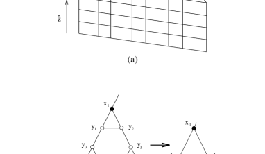
FIG. 1.: (a) Schematic diagram of the lattice with the iteration number $n$ = 2 and $L$ = 5. Each vertex is a lattice site of the Hamiltonian given by Eq. (1). (b) Schematic diagram of the decimation process. The amplitudes of the sites represented by the empty circles are eliminated to modify the forms of the equations for the sites represented by the solid circles.

FIG. 2.: Log-log plot of the renormalized localization length along the Sierpinski gasket as a function of $L$ for various values of $W$. The uncertainty of each data point is less than the symbol size.

FIG. 3.: Scaling behavior of $\log(\lambda_{xy}/L)$ versus $(W-W_{c})\$ $L^{1/\nu}$ with $W_{c}$ = 5.79 and $\nu$ = 2.92.

REFERENCES

- [1] R. N. Bhatt, P. Wölfle and T. V. Ramakrishnan, Phys. Rev. B 32, 569 (1985).
- [2] Qiming Li, C. M. Soukoulis, E. N. Economou and G. S. Grest, Phys. Rev. 40, 2825 (1989).
- [3] A. G. Rojo and K. Levin, Phys. Rev. B 48, 16861 (1993), and references therein.
- [4] A. A. Abrikosov, Phys. Rev. B 50, 1415 (1994).
- [5] W. Xue, P. Sheng, Q. J. Chu and Z. Q. Zhang, Phys. Rev. Lett. 63, 2837 (1989); Phys. Rev. B 42, 4613 (1990); Q. J. Chu and Z. Q. Zhang, Phys. Rev. B 48, 10761 (1993).
- [6] I. Zambetaki, Qiming Li, E. N. Economou and C. M. Soukoulis, Phys. Rev. Lett. 76, 3614 (1996).
- [7] Y. Shi and C. Gong, Phys. Rev. E 49, 99 (1994).
- [8] M. Schreiber and H. Grussbach, Phys. Rev. Lett. 76, 1687 (1996).
- [9] H. Grussbach, Ph.D. thesis, Johannes Gutenberg-Universität, 1995 (unpublished).
- [10] See B. Kramer and A. MacKinnon, Rep. Prog. Phys. 56, 1469 (1993) and references therein.