Spectral functions of the 1D Hubbard model in the $U\rightarrow+\infty$ limit: How to use the factorized wave-function

Abstract

We give the details of the calculation of the spectral functions of the 1D Hubbard model using the spin-charge factorized wave-function for several versions of the $U\rightarrow+\infty$ limit. The spectral functions are expressed as a convolution of charge and spin dynamical correlation functions. A procedure to evaluate these correlation functions very accurately for large systems is developed, and analytical results are presented for the low energy region. These results are fully consistent with the conformal field theory. We also propose a direct method of extracting the exponents from the matrix elements in more general cases.

I Introduction

After the recent photoemission experiments[2, 3] on quasi one-dimensional materials, the need of understanding the dynamical spectral functions of strongly correlated electron systems has arised. While the low energy behavior is usually well described within the framework of the Luttinger liquid theory,[4, 5, 6] the experimentally relevant higher energies ($\approx 100$ meV) can be calculated for example by diagonalizing small clusters[7] or by Quantum Monte-Carlo calculations.[8] Unfortunately, both methods have limitations either given by the small size of the system or by statistical errors and use of analytic continuation. Even for the Bethe-Ansatz solvable models, where the excitation spectra can be calculated, the problematic part of calculating the matrix elements remains: The wave functions are required, and they are simply too complicated. There is, however, a special class of models, where the evaluation of the matrix elements is made possible through a relatively simple factorized form of the wave-function, and some results were already published by Sorella and Parolla[9] for the insulating half-filled case and by the authors[10, 11] away from half-filling.

The dynamical, zero temperature one-particle spectral functions can be defined as the imaginary parts of the time ordered Green’s function:

$\displaystyle\begin{array}[]{lc}A(k,\omega)=\displaystyle{\frac{1}{\pi}}{\rm Im}G(k,\omega),&\mbox{for $\omega>\mu$};\\ &\\ B(k,\omega)=-\displaystyle{\frac{1}{\pi}}{\rm Im}G(k,\omega),&\mbox{for $\omega<\mu$}.\\ \end{array}$

$A(k,\omega)$ is measured in angular resolved inverse photoemission experiments and can be calculated from the Lehmann representation:

$\displaystyle A(k,\omega)=\sum_{f,\sigma}\left|\langle f,N\!+\!1|a^{\dagger}_{k,\sigma}|0,N\rangle\right|^{2}\delta(\omega\!-\!E^{N+1}_{f}\!+\!E^{N}_{0}),$

while $B(k,\omega)$ is measured in the angular resolved photoemission experiments and is given by:

$\displaystyle B(k,\omega)=\sum_{f,\sigma}\left|\langle f,N\!-\!1|a^{\phantom{\dagger}}_{k,\sigma}|0,N\rangle\right|^{2}\delta(\omega\!-\!E^{N}_{0}\!+\!E^{N-1}_{f}).$

Here $N$ is the number of electrons, $f$ denotes the final states and $a_{k,\sigma}$ destroys an electron with momentum $k$ and spin $\sigma$. If the spectral functions are known, the time ordered Green’s function can be obtained from

$$G(k,\omega)=\int_{\mu}^{+\infty}{\rm d}\omega^{\prime}\frac{A(k,\omega^{\prime})}{\omega\!-\!\omega^{\prime}\!+\!i\delta}+\int_{-\infty}^{\mu}{\rm d}\omega^{\prime}\frac{B(k,\omega^{\prime})}{\omega\!-\!\omega^{\prime}\!-\!i\delta}.$$ (1)

The special models for which the matrix elements can be calculated are:

i) The Hubbard model, defined as usual:

$$H=-t\sum_{i,\sigma}\left(a^{\dagger}_{i+1,\sigma}a^{\phantom{\dagger}}_{i,\sigma}+h.c.\right)+U\sum_{i}n_{i,\uparrow}n_{i,\downarrow},$$ (2)

in the limit $U/t\rightarrow+\infty$;

ii) The anisotropic $t-J$ model

$$H_{tJ} = -t\sum_{i,\sigma}(\tilde{a}_{i,\sigma}^{\dagger}\tilde{a}_{i+1,\sigma}^{\vphantom{\dagger}}+{\rm h.c.})$$ (4)

$$+\sum_{i}\sum_{\alpha=x,y,z}J^{\alpha}\left(S_{i}^{\alpha}S_{i+1}^{\alpha}-\frac{1}{4}\delta_{\alpha,z}n_{i}n_{i+1}\right),$$

in the limit $J^{\alpha}\rightarrow 0$, where $\tilde{a}_{i,\sigma}$ are the usual projected operators. Actually, the Hubbard model in the large $U$ limit can be mapped onto a strong coupling model usually identified as the $t-J$ model plus three-site terms using a canonical transformation,[12, 13] where $J=4t^{2}/U$ is small;

iii) An extension of the $t-J$ model first proposed by Xiang and d’Ambrumenil,[14] defined by the Hamiltonian

$${\cal H} = -t\sum_{i,\sigma}\left(\tilde{a}^{\dagger}_{i,\sigma}\tilde{a}^{\phantom{\dagger}}_{i+1,\sigma}+h.c.\right)$$ (6)

$$+\sum_{i>j}\sum_{\alpha=x,y,z}J^{\alpha}\left(S_{i}^{\alpha}S_{i+j}^{\alpha}-\frac{1}{4}\delta_{\alpha,z}n_{i}n_{i+j}\right){\cal P}_{i,j},$$

where ${\cal P}_{i,j}=\prod_{j^{\prime}=1}^{j-1}(1\!-\!n_{i+j^{\prime}})$ in the exchange part of the Hamiltonian ensures that two spins interact as long as there is no other spin between them. The motivation to study this model is that, unlike the infinite $U$ Hubbard model, there is a finite energy $J$ associated with spin fluctuations, and this will give us useful indications about the finite $U$ Hubbard model.

From the models defined above, the Hubbard model is the most relevant one. It plays a central role as the generic model of strongly correlated electron systems. Even though it is comparatively simple, it is very difficult to solve except for the one dimensional case, where it is solvable by Bethe Ansatz.[15] Unfortunately, the Bethe ansatz solution is not convenient for direct computation of spectral functions, therefore an alternative approach was needed. In the limit of small $U$ one can use the renormalization group[16] to show that the Hubbard model belongs to the universality class of the Tomonaga-Luttinger model,[17] usually referred to as Luttinger-liquid.[18] The Luttinger liquids are characterized by power-law decay of correlation functions, and nonexistence of quasiparticles.[19] The underlying conformal field theory can be used to relate the exponents to finite-size corrections of the energy and momentum.[20, 21, 22, 23] This gives consistent results not only with the renormalization group in the weak coupling regime,[24] but also with the special case of $U/t\rightarrow+\infty$, where the exponents of the static correlations could be obtained using a factorized wave function.[25, 26, 27]

Actually, the spin-charge factorized wave function also describes the excited states as well,[28] and it can be used to calculate the dynamical spectral functions as well. The spectral functions obtained in this way are very educative and in some sense, unexpected. For example, it turns out that the spectrum contains remnants of bands[11] crossing the Fermi energy at $3k_{F}$ - the so called shadow bands. Also it gives information on the applicability of the power-law Luttinger liquid correlation function.[10] The aim of this paper is not only to give the details of the calculation, that can be useful for other correlation functions, but also to present some new results on the low energy behavior of the charge and spin part (both for the isotropic Heisenberg and XY spin model).

The paper is organized as follows: In Section II we review the factorized wave function and in Section III we show how the spectral functions can be given as a convolution of spin and charge parts. Sections IV and V are devoted to the detailed analysis of the charge and spin parts. The relation to the results obtained from the finite-size corrections and conformal field theory is discussed in Section VI. Finally, in Section VII we present our conclusions.

II The factorized wave function

It has been shown,[25, 28] by using the Bethe ansatz solution, that the ground state wave function of the Hubbard model in the $U\rightarrow+\infty$ limit can be constructed as a product of a spinless fermion wave function $|\psi\rangle$ and a squeezed spin wave function $|\chi\rangle$. This can be alternatively seen using perturbational arguments[25] and then extended to the $t-J$ model in the $J\rightarrow 0$ limit. Moreover, the wave function of the excited states are also factorized:[9, 28]

$$|N\rangle=|\psi^{N}_{L,Q}(\{{\cal I}\})\rangle\otimes|\chi^{N_{\downarrow}}_{N}(Q,\tilde{f}_{Q})\rangle.$$ (7)

The spinless fermion wave function $|\psi\rangle$ describes the charges and is an eigen function of $N$ noninteracting spinless fermions on $L$ sites with momenta

$$k_{j}L=2\pi{\cal I}_{j}+Q,$$ (8)

where the ${\cal I}_{j}$ are integer quantum numbers and $j=1,2,\dots N$. The charge part is not fully decoupled from the spin wave function $|\chi\rangle$, as the momentum $Q=2\pi{\cal J}/N$ (${\cal J}=0,1,\dots,N-1$ ) of the spin wave function imposes a twisted boundary condition on the spinless fermion wave-function (each fermion hopping from site $L-1$ to site $0$ will acquire a phase $e^{iQ}$) to ensure periodic boundary conditions for the original problem. The energy of the charge part is

$$E^{N}_{c}=-2t\sum_{j=1}^{N}\cos k_{j},$$ (9)

and the momentum reads $P^{N}_{c}=\sum_{j=1}^{N}k_{j}$, or, using Eq. (8):

$$P^{N}_{c}=\frac{2\pi}{L}\sum_{j=1}^{N}{\cal I}_{j}+\frac{N}{L}Q=\frac{2\pi}{L}\left(\sum_{j=1}^{N}{\cal I}_{j}+{\cal J}\right).$$ (10)

On the other hand, the spin wave functions $|\chi\rangle$ are characterized by the number of down spins $N_{\downarrow}$, the total momentum $Q$, and the quantum number $\tilde{f}_{Q}$ within the subspace of momentum $Q$. They are eigenfunctions of the Heisenberg Hamiltonian

$$H_{s}=\sum_{i=1}^{N}\sum_{\alpha=x,y,z}\tilde{J}^{\alpha}\left(S_{i}^{\alpha}S_{i+1}^{\alpha}-\frac{1}{4}\delta_{\alpha,z}\right).$$ (11)

with eigenenergies $E_{s}$. $\tilde{J}^{\alpha}$ depends on the actual charge wave function $|\psi\rangle$. In the case of the $U\rightarrow+\infty$ Hubbard model,

$$\tilde{J}=\frac{2t^{2}}{U}\frac{1}{N}\sum_{i,\delta=\pm 1}\langle\psi|n_{i}n_{i+\delta}-b^{\dagger}_{i+\delta}n_{i}b^{\phantom{\dagger}}_{i-\delta}|\psi\rangle,$$ (12)

where $b^{\dagger}_{j}$ and $b^{\phantom{\dagger}}_{j}$ are the operators of spinless fermions at site $j$. For the ground state $|\psi^{\rm GS}\rangle$ it reads $\tilde{J}^{\alpha}=n(4t^{2}/U)[1-\sin(2\pi n)/(2\pi n)]$, where $n=N/L$ is the density.

For the $t-J$ model:

$$\tilde{J}^{\alpha}=J^{\alpha}\sum_{i}\langle\psi|n_{i}n_{i+j}|\psi\rangle,$$ (13)

and for the ground state $\tilde{J}^{\alpha}=J^{\alpha}n[1-\sin^{2}(\pi n)/(\pi n)^{2}]$. For the model of Xiang and d’Ambrumenil $\tilde{J}^{\alpha}=nJ^{\alpha}$ and is independent of the charge part. The energy of the factorized wave function is then given as the sum of the charge and spin energies, with the assumption that the correct $\tilde{J}$ is chosen. If $U\rightarrow+\infty$ or $J\rightarrow 0$, then the spectrum collapses and we can assume all the spin states degenerate, simplifying considerably some of the calculations to be presented later.

Furthermore, we choose $N$ to be of the form $4l+2$ ($l$ integer), when the ground state is unique. Then in the ground-state the spinless fermion wave-function $|\psi_{L}^{N,\rm GS}\rangle$ is described by the quantum numbers $Q=\pi$ and $\{{\cal I}\}=\{-N/2,\dots,N/2-2,N/2-1\}$, so that the distribution of the $k_{j}$’s is symmetric around the origin and we choose the spin part as the ground-state of the Heisenberg model according to Ogata and Shiba’s prescription.[25] This choice of the spin wave function makes the difference between the $U\rightarrow+\infty$ and $U=+\infty$ (the so called $t$ model) limits.

The price we have to pay for such a simple wave function is that the representation of real fermion operators $a^{\dagger}_{j,\sigma}$ in the new basis becomes complicated. As a first step, we can write $a^{\dagger}_{j,\sigma}$ as $a^{\dagger}_{j,\sigma}=a^{\dagger}_{j,\sigma}(1-n_{j,\bar{\sigma}})+a^{\dagger}_{j,\sigma}n_{j,\bar{\sigma}}$, where $a^{\dagger}_{j,\sigma}(1-n_{j,\bar{\sigma}})$ creates a fermion at an unoccupied site and the $a^{\dagger}_{j,\sigma}n_{j,\bar{\sigma}}$ adds a fermion at an already occupied site, thus creating a doubly occupied site. $\bar{\sigma}$ means the spin state opposite to $\sigma$. This latter process gives contributions to the spectral functions in the upper Hubbard band, $A^{\rm UHB}(k,\omega)$ which can be calculated in a similar way, but we will not address this issue in the present paper.

Next, we define the operators $\hat{Z}^{\dagger}_{i,\sigma}$ and $\hat{Z}^{\phantom{\dagger}}_{i,\sigma}$ acting on the spin part of the wave function: The $\hat{Z}^{\dagger}_{i,\sigma}$ adds a spin $\sigma$ to the beginning of the spin wave function $|\chi_{N}\rangle$ if $i=0$, or inserts a spin $\sigma$ after skipping the first $i$ spins, and makes it $N+1$ long, e.g.: $\hat{Z}^{\dagger}_{0,\sigma}|\uparrow\downarrow\rangle=|\sigma\uparrow\downarrow\rangle$ and $\hat{Z}^{\dagger}_{1,\sigma}|\uparrow\downarrow\rangle=|\uparrow\sigma\downarrow\rangle$. The $\hat{Z}_{i,\sigma}$ is defined as the adjoint operator of $\hat{Z}^{\dagger}_{i,\sigma}$, i.e. it removes a spin from site $i$.

Then, to create a fermion at the empty site $j=0$, we need to create one spinless fermion with operator $b^{\dagger}_{0}$ and to add a spin $\sigma$ to the spin wave function with operator $\hat{Z}^{\dagger}_{0,\sigma}$:

$$a^{\dagger}_{0,\sigma}(1-n_{0,\bar{\sigma}})=\hat{Z}^{\dagger}_{0,\sigma}b^{\dagger}_{0}.$$ (14)

The apparent simplicity is lost for $a^{\dagger}_{1,\sigma}$. Then, apart from creating a spinless fermions with $b^{\dagger}_{1}$ in the charge part, we have to consider the following two possibilities: either the $j=0$ site is empty, and with $a^{\dagger}_{1,\sigma}$ we create a spin at the beginning of the spin wave function with $\hat{Z}^{\dagger}_{0,\sigma}$; or it is occupied, and we insert a spin between the first and second spin in $|\chi\rangle$ with $\hat{Z}^{\dagger}_{1,\sigma}$. So we end up with

$\displaystyle a^{\dagger}_{1,\sigma}(1-n_{1,\bar{\sigma}})=\left[(1-n_{0})\hat{Z}^{\dagger}_{0,\sigma}+n_{0}\hat{Z}^{\dagger}_{1,\sigma}\right]b^{\dagger}_{1}.$

Obviously we choose the $j=0$ in further calculations for its simplicity. However, one can show that the final result does not depend on this special choice and the translational invariance is preserved even for these complicated operators.

III Spectral Functions

To use the factorized wave functions in the calculation of the spectral function it is more convenient to transfer the $k$ dependence from the $a^{\dagger}_{k,\sigma}$ operator to the final state:

$$A(k,\omega) = \sum_{f,\sigma}L\left|\langle f,N\!+\!1|a^{\dagger}_{0,\sigma}|0,N\rangle\right|^{2}$$ (16)

$$\times\delta(\omega\!-\!E^{N+1}_{f}\!+\!E^{N}_{0})\delta_{k,P^{N+1}_{f}\!-\!P_{0}^{N}}$$

and

$$B(k,\omega) = \sum_{f,\sigma}L\left|\langle f,N\!-\!1|a^{\phantom{\dagger}}_{0,\sigma}|0,N\rangle\right|^{2}$$ (18)

$$\times\delta(\omega\!-\!E^{N}_{0}\!+\!E^{N-1}_{f})\delta_{k,P_{0}^{N}\!-\!P^{N-1}_{f}},$$

where the momenta of the final states are $P^{N\pm 1}_{f}$.

As we already pointed out, the addition of an electron to the ground state can result in a final state with or without a doubly occupied state. Correspondingly, the spectral function has contributions from the upper and lower Hubbard bands: $A(k,\omega)=A^{\rm UHB}(k,\omega)+A^{\rm LHB}(k,\omega)$. We will now consider $A^{\rm LHB}(k,\omega)$ only. From Eqs. (7) and (14) we get the following convolution as a consequence of the wave function factorization:

$$A^{\rm LHB}(k,\omega)=\sum_{Q,\omega^{\prime},\sigma}C_{\sigma}(Q,\omega^{\prime})A_{Q}(k,\omega-\omega^{\prime}),$$ (19)

and similarly for $B(k,\omega)$:

$$B(k,\omega)=\sum_{Q,\omega^{\prime},\sigma}D_{\sigma}(Q,\omega^{\prime})B_{Q}(k,\omega-\omega^{\prime}).$$ (20)

$A_{Q}(k,\omega)$ and $B_{Q}(k,\omega)$ depend on the spinless fermion wave function only:

$$A_{Q}(k,\omega) = L\sum_{\{I\}}\left|\langle\psi_{L,Q}^{N+1}(\{I\})|b^{\dagger}_{0}|\psi_{L,\pi}^{N,{\rm GS}}\rangle\right|^{2}$$ (22)

$$\times\delta(\omega-E^{N+1}_{f,c}+E^{N}_{{\rm GS},c})\delta_{k,P^{N+1}_{f,c}\!-\!P^{N}_{{\rm GS},c}},$$

$$B_{Q}(k,\omega) = L\sum_{\{I\}}\left|\langle\psi_{L,Q}^{N-1}(\{I\})|b^{\phantom{\dagger}}_{0}|\psi_{L,\pi}^{N,{\rm GS}}\rangle\right|^{2}$$ (24)

$$\times\delta(\omega-E^{N}_{{\rm GS},c}+E^{N-1}_{f,c})\delta_{k,P^{N}_{{\rm GS},c}\!-\!P^{N-1}_{f,c}},$$

and they are discussed in more detail in the next section (Sec. IV).

On the other hand, $C_{\sigma}(Q,\omega)$ and $D_{\sigma}(Q,\omega)$ are determined by the spin wave function only:

$$C_{\sigma}(Q,\omega) = \sum_{\tilde{f}_{Q}}\left|\langle\chi_{N+1}(Q,\tilde{f}_{Q})|\hat{Z}^{\dagger}_{0,\sigma}|\chi_{N}^{\rm GS}\rangle\right|^{2}$$ (26)

$$\times\delta(\omega-E^{N+1}_{f,s}+E^{N}_{{\rm GS},s}),$$

$$D_{\sigma}(Q,\omega) = \sum_{\tilde{f}_{Q}}\left|\langle\chi_{N-1}(Q,\tilde{f}_{Q})|\hat{Z}_{0,\sigma}|\chi_{N}^{\rm GS}\rangle\right|^{2}$$ (28)

$$\times\delta(\omega-E^{N}_{{\rm GS},s}+E^{N-1}_{f,s}),$$

and are analyzed in Sec. V. Although we do not present it here, a similar analysis can be made for $A^{\rm UHB}(k,\omega)$.

In Eqs. (19) and (20) the simple addition of the spin and charge energies is assumed. Strictly speaking, this is only valid for the $U\rightarrow+\infty$, $J\rightarrow 0$ and the model of Xiang and d’Ambrumenil for any $J$. In the other cases the dependence of $\tilde{J}$ on the charge wave function should be explicitly taken into account. Still, it is a reasonable approximation, as the important matrix elements will come from exciting a few particle-hole excitations only, which will give finite-size corrections to $\tilde{J}$ in the thermodynamic limit. Furthermore, we are neglecting the $t^{2}/U$ corrections to the effective operators[13] and to the wave functions.

The momentum distribution function, $n_{k}=\langle a^{\dagger}_{k}a^{\phantom{\dagger}}_{k}\rangle$ can be calculated from the spectral function as $n_{k}=\int B(k,\omega)d\omega$, leading to a similar expression as used by Pruschke and Shiba:[29]

$$n_{k}=\sum_{Q}B_{Q}(k)D(Q),$$ (29)

where $B_{Q}(k)=\int B_{Q}(k,\omega)d\omega$ and similarly $D(Q)=\int D(Q,\omega)d\omega$.

The local spectral function $A(\omega)=\frac{1}{L}\sum_{k}A(k,\omega)$ is given by

$$A(\omega)=\sum_{Q,\omega^{\prime},\sigma}C_{\sigma}(Q,\omega^{\prime})A_{Q}(\omega-\omega^{\prime}),$$ (30)

where $A_{Q}(\omega)=\frac{1}{L}\sum_{k}A_{Q}(k,\omega)$. Similar equation holds for $B(\omega)$.

IV About $A_{Q}(k,\omega)$ and $B_{Q}(k,\omega)$

To calculate $A_{Q}(k,\omega)$ and $B_{Q}(k,\omega)$ defined in Eq. (24), we need to evaluate matrix elements like $\langle\psi_{L,Q}^{N+1}(\{I\})|b^{\dagger}_{0}|\psi_{L,Q^{\prime}}^{N,\rm GS}\rangle$, where the two states have different boundary conditions. In the ground state $Q^{\prime}=\pi$, but we will not specify $Q^{\prime}$ yet. To calculate these matrix elements, we need the following anti-commutation relation:

$$\bigl{\{}b^{\dagger}_{k^{\prime}},b^{\phantom{\dagger}}_{k}\bigr{\}} = \frac{1}{L}\sum_{j,j^{\prime}}e^{ik^{\prime}j^{\prime}-ikj}\bigl{\{}b^{\dagger}_{j^{\prime}},b^{\phantom{\dagger}}_{j}\bigr{\}}$$ (31)

$$= \frac{1}{L}e^{-i(k^{\prime}-k)/2}e^{i(Q^{\prime}-Q)/2}\frac{\sin([Q^{\prime}-Q]/2)}{\sin([k^{\prime}-k]/2)}.$$ (32)

where $k$ and $k^{\prime}$ are wave-vectors with phase shift $Q/L$ and $Q^{\prime}/L$, respectively, see Eq. (8). For $Q\rightarrow Q^{\prime}$ the anti-commutation relation is the usual one: $\bigl{\{}b^{\dagger}_{k^{\prime}},b^{\phantom{\dagger}}_{k}\bigr{\}}=\delta_{k,k^{\prime}}$, while for $Q\neq Q^{\prime}$ the overall phase shift $(Q-Q^{\prime})/L$ due to momentum transfer $Q-Q^{\prime}$ to the spin degrees of freedom gives rise to the Anderson’s orthogonality catastrophe.[30] Then a typical overlap $\langle 0|b^{\phantom{\dagger}}_{k_{N}}\dots b^{\phantom{\dagger}}_{k_{2}}b^{\phantom{\dagger}}_{k_{1}}b^{\dagger}_{k^{\prime}_{1}}b^{\dagger}_{k^{\prime}_{2}}\dots b^{\dagger}_{k^{\prime}_{N}}|0\rangle$, where $|0\rangle$ is the vacuum state, is given by the following determinant:

$\displaystyle\left|\begin{array}[]{cccc}\bigl{\{}b_{k^{\prime}_{1},k_{1}}\bigr{\}}&\bigl{\{}b_{k^{\prime}_{1},k_{2}}\bigr{\}}&\dots&\bigl{\{}b_{k^{\prime}_{1},k_{N}}\bigr{\}}\cr\bigl{\{}b_{k^{\prime}_{2},k_{1}}\bigr{\}}&\bigl{\{}b_{k^{\prime}_{2},k_{2}}\bigr{\}}&\dots&\bigl{\{}b_{k^{\prime}_{2},k_{N}}\bigr{\}}\cr\vdots&\vdots&&\vdots\cr\bigl{\{}b_{k^{\prime}_{N},k_{1}}\bigr{\}}&\bigl{\{}b_{k^{\prime}_{N},k_{2}}\bigr{\}}&\dots&\bigl{\{}b_{k^{\prime}_{N},k_{N}}\bigr{\}}\end{array}\right|.$

Replacing the anticommutator, the determinant above becomes

$$L^{-N}e^{i(Q^{\prime}-Q)N/2}\prod_{j}e^{-i(k^{\prime}_{j}-k_{j})/2}\sin^{N}\frac{Q^{\prime}-Q}{2}$$ (33)

$$\times\left|\begin{array}[]{cccc}\sin^{-1}\frac{k^{\prime}_{1}-k_{1}}{2}&\sin^{-1}\frac{k^{\prime}_{1}-k_{2}}{2}&\dots&\sin^{-1}\frac{k^{\prime}_{1}-k_{N}}{2}\cr&&&\cr\sin^{-1}\frac{k^{\prime}_{2}-k_{1}}{2}&\sin^{-1}\frac{k^{\prime}_{2}-k_{2}}{2}&\dots&\sin^{-1}\frac{k^{\prime}_{2}-k_{N}}{2}\cr&&&\cr\vdots&\vdots&&\vdots\cr&&&\cr\sin^{-1}\frac{k^{\prime}_{N}-k_{1}}{2}&\sin^{-1}\frac{k^{\prime}_{N}-k_{2}}{2}&\dots&\sin^{-1}\frac{k^{\prime}_{N}-k_{N}}{2}\end{array}\right|.$$ (41)

This determinant is very similar to the Cauchy determinant (there the elements are $1/(k-k^{\prime})$ instead of $1/\sin(k-k^{\prime})$) and it can be expressed as a product,[31] so for the overlap we get:

$$\pm L^{-N}e^{i(Q^{\prime}-Q)N/2}\sin^{N}\frac{Q^{\prime}-Q}{2}\prod_{j}e^{-i(k^{\prime}_{j}-k_{j})/2}$$ (42)

$$\times \prod_{j>i}\sin\frac{k_{j}-k_{i}}{2}\prod_{j>i}\sin\frac{k^{\prime}_{j}-k^{\prime}_{i}}{2}\prod_{i,j}\sin^{-1}\frac{k^{\prime}_{i}-k_{j}}{2},$$ (43)

where the sign $+$ is for $N=1,4,5,8,9,..$ and $-$ for $N=2,3,6,7,..$.

Now we turn back to the $A_{Q}(k,\omega)$. The matrix elements in Eq. (24) are

$$L\bigl{|}\langle\psi^{N+1}_{L,Q}(\{{\cal I}\})|b^{\dagger}_{0}|\psi_{L,Q^{\prime}}^{N,\rm GS}\rangle\bigr{|}^{2} = \Bigl{|}\sum_{q^{\prime}}\langle\psi^{N+1}_{L,Q}(\{{\cal I}\})|b^{\dagger}_{q^{\prime}}|\psi^{N,\rm GS}_{L,Q^{\prime}}\rangle\Bigr{|}^{2}$$ (44)

$$= L^{-2N}\sin^{2N}\frac{Q^{\prime}-Q}{2}\prod_{j>i}\sin^{2}\frac{k_{j}-k_{i}}{2}\prod_{j>i}\sin^{2}\frac{k^{\prime}_{j}-k^{\prime}_{i}}{2}\prod_{i,j}\sin^{-2}\frac{k^{\prime}_{i}-k_{j}}{2},$$ (45)

where $q^{\prime}$ is a wave vector with phase shift $Q^{\prime}/L$. Here we have used that

$$\Biggl{|}\sum_{q^{\prime}}e^{iq^{\prime}/2}\prod_{i^{\prime}=1}^{N}\sin\frac{k^{\prime}_{i^{\prime}}\!-\!q^{\prime}}{2}\prod_{i=1}^{N+1}\sin^{-1}\frac{k_{i}\!-\!q^{\prime}}{2}\Biggr{|}^{2}$$ (46)

$$=L^{2}\sin^{-2}\frac{Q^{\prime}\!-\!Q}{2}$$ (47)

holds, independently of the actual quantum numbers $\{{\cal I}\}$ and $\{{\cal I^{\prime}}\}$.

Similarly, for the matrix elements in $B_{Q}(k,\omega)$ we get:

$$L\left|\langle\psi^{N-1}_{L,Q}(\{I\})|b^{\phantom{\dagger}}_{0}|\psi_{L,Q^{\prime}}^{N,\rm GS}\rangle\right|^{2}=L^{-2N+2}\sin^{2N-2}\frac{Q^{\prime}\!-\!Q}{2}$$ (48)

$$\times\prod_{j>i}\sin^{2}\frac{k_{j}\!-\!k_{i}}{2}\prod_{j>i}\sin^{2}\frac{k^{\prime}_{j}\!-\!k^{\prime}_{i}}{2}\prod_{i,j}\sin^{-2}\frac{k^{\prime}_{i}\!-\!k_{j}}{2}.$$ (49)

We are now ready to calculate the spectral functions numerically. One has to generate the quantum numbers ${\cal I}_{j}$, and evaluate the energy, momentum and the expressions above.

From now on, we will consider $Q^{\prime}=\pi$.

First of all, it turns out that the following sum rules are satisfied for every $Q$:

$$\int_{-\pi}^{\pi}\frac{dk}{2\pi}\int_{-\infty}^{\infty}d\omega A_{Q}(k,\omega) = 1-n,$$ (50)

$$\int_{-\pi}^{\pi}\frac{dk}{2\pi}\int_{-\infty}^{\infty}d\omega B_{Q}(k,\omega) = n.$$ (51)

In the absence of the Anderson orthogonality catastrophe, when $Q=Q^{\prime}=\pi$, the contribution to the spectral functions comes from one particle-hole excitations only, and the spectral functions are nothing but the familiar $\delta(\omega+2t\cos k)$. This is not true any more when we consider $Q\neq\pi$. In that case we get contributions from many particle-hole excitations as well. The largest weight comes from the one particle-hole excitations, and increasing the number of excited holes, the additional weight decreases rapidly. Although from Eq. (45) we can calculate the matrix elements numerically for all the excitations of the final state, its application is limited to small system sizes (typically $L<30$). It is due to the fact that the time required to generate all the possible states (quantum numbers ${\cal I}$) is growing exponentially. Therefore, in some of the calculations we take into account up to three particle-hole excitations only. In Table. I we give the total sum rule for small sizes in a calculation where we took into account up to one, two and three particle-hole excitations. We can see that the missing weight is really small in the approximation that includes up to three particle-hole excitations in the final state. So, if we restrict ourselves to a finite number of particle-hole excitations and introduce the function

$$g({\cal I}) = \prod_{{\cal I^{\prime}}=-N/2\atop{{\cal I^{\prime}}\neq{\cal I}}}^{N/2}\sin^{2}\frac{\pi}{L}({\cal I}\!-\!{\cal I^{\prime}})$$ (53)

$$\times\prod_{{\cal I^{\prime\prime}}=-N/2}^{N/2-1}\sin^{-2}\left([{\cal I}\!-\!{\cal I^{\prime\prime}}]\frac{\pi}{L}+\frac{Q\!-\!\pi}{2L}\right),$$

the calculation of the spectral weight becomes simple. The weight of the peak corresponding to a one particle-hole excitation can be given as:

$$A_{Q}({\cal I}^{p},{\cal I}^{h})=\frac{g({\cal I}^{p})}{g^{(}{\cal I}^{h})}\frac{1}{\sin^{2}([{\cal I}^{h}-{\cal I}^{p}]\frac{\pi}{L})}A_{Q}^{(0,0)},$$ (54)

where we have removed the quantum number ${\cal I}^{h}$ (hole) from and added ${\cal I}^{p}$ (particle) to the set $\{{\cal I}\}$ of the ground-state of $N\pm 1$ fermions, so that the momentum of the final state is $P^{N+1}_{f}=k^{p}-k^{h}+P_{\rm GS}^{N+1}$ and the energy is $E^{N+1}_{f}=E^{N+1}_{\rm GS}-2t\cos k^{p}+2t\cos k^{h}$, where the $P_{\rm GS}^{N+1}=(N+1)Q/L$ is the momentum of the ground state. Furthermore, $A_{Q}^{(0,0)}$ is the overlap between the $N$ electron ground state with boundary condition $\pi$ and the $N+1$ electron ground state with boundary condition $Q$, and will be discussed later.

Similarly, for the two particle-hole excitations we get:

$$A_{Q}({\cal I}^{p}_{1},{\cal I}^{p}_{2},{\cal I}^{h}_{1},{\cal I}^{h}_{2})=\frac{g({\cal I}^{p}_{1})g({\cal I}^{p}_{2})}{g({\cal I}^{h}_{1})g({\cal I}^{h}_{2})}\frac{\sin^{2}([{\cal I}^{h}_{1}\!-\!{\cal I}^{h}_{2}]\frac{\pi}{L})\sin^{2}([{\cal I}^{p}_{1}\!-\!{\cal I}^{p}_{2}]\frac{\pi}{L})}{\sin^{2}([{\cal I}^{p}_{1}\!-\!{\cal I}^{h}_{1}]\frac{\pi}{L})\sin^{2}([{\cal I}^{p}_{1}\!-\!{\cal I}^{h}_{2}]\frac{\pi}{L})\sin^{2}([{\cal I}^{p}_{2}\!-\!{\cal I}^{h}_{1}]\frac{\pi}{L})\sin^{2}([{\cal I}^{p}_{2}\!-\!{\cal I}^{h}_{2}]\frac{\pi}{L})}A_{Q}^{(0,0)}$$ (55)

with energy and momentum

$$E^{N+1} = E^{N+1}_{\rm GS}-2t\left(\cos k^{p}_{1}+\cos k^{p}_{2}-\cos k^{h}_{1}-\cos k^{h}_{2}\right),$$ (56)

$$P^{N+1} = k^{p}_{1}+k^{p}_{2}-k^{h}_{1}-k^{h}_{2}+P^{N+1}_{\rm GS}.$$ (57)

The corresponding equations for three or more particle-hole excitations are similar to those above, but since they are long, we do not give them here.

A typical plot of $A_{Q}(k,\omega)$ is shown in Fig. 1. We choose $Q=\pi/2$, which is halfway between the symmetric $Q=0$ and the trivial $Q=\pi$ case. In the figure we can see the singularity near the Fermi energy, furthermore the weights are distributed on a cosine- like band. To make it more clear, in Fig. 2 we show the support of $A_{Q}(k,\omega)$ and the distribution of the weights.

A The weight of the lowest peak

Now, what can we say about $A_{Q}^{(0,0)}$, the weight of the lowest peak? In the ground state the quantum numbers ${\cal I}_{j}$ and ${\cal I}_{j}^{\prime}$ are densely packed, and from Eq. (45) we get

$$A_{Q}^{(0,0)} = \frac{\cos^{2N}(Q/2)}{L^{2N}}\prod_{j=1}^{N}\left[\sin^{2}\frac{\pi j}{L}\right]^{2N+1-2j}$$ (59)

$$\times\prod_{j=1}^{N}\left[\sin^{2}\frac{(2j\!-\!1)\pi\!+\!Q}{2L}\sin^{2}\frac{(2j\!-\!1)\pi\!-\!Q}{2L}\right]^{j-N-1}$$

From this we can conclude that $A_{Q}^{(0,0)}$ is an even function of $Q$ and $A_{\pi}^{(0,0)}=1$. We are not able to give a closed formula for the sum. However, very useful information can be obtained by noticing that

$\displaystyle\frac{A_{Q+\pi}^{(0,0)}}{A_{Q-\pi}^{(0,0)}}=\prod_{j=1}^{N}\frac{\sin^{2}\frac{2j\pi-Q}{2L}}{\sin^{2}\frac{2j\pi+Q}{2L}},$

and in the thermodynamic limit,

$\displaystyle\frac{A_{Q+2\pi}^{(0,0)}A_{Q-2\pi}^{(0,0)}}{\left(A_{Q}^{(0,0)}\right)^{2}}=\frac{(\pi^{2}-Q^{2})^{2}}{(2L\sin\pi n)^{4}}\left[1-\frac{2\pi}{L}\cot\pi n+O(L^{-2})\right].$

Here the $Q$ is extended outside the Brillouin zone. Now it is straightforward to get the size- and filling-dependence of $A_{Q}^{(0,0)}$:

$$A_{Q}^{(0,0)}=\frac{f(Q)}{(L\sin\pi n)^{\alpha_{Q}}}\left[1-\alpha_{Q}\frac{\pi}{2L}\cot\pi n+O(L^{-2})\right],$$ (60)

where

$$\alpha_{Q}=\frac{1}{2}\left(\frac{Q}{\pi}\right)^{2}-\frac{1}{2}.$$ (61)

Eq. (60) is also valid for $B_{Q}^{(0,0)}$, apart from the sign in the $1/L$ correction.

The $f(Q)$ is an even function of $Q$, $f(\pi)=1$, and it satisfies the second order recurrence equation

$\displaystyle\frac{f(Q+2\pi)f(Q-2\pi)}{f^{2}(Q)}=\frac{(\pi^{2}-Q^{2})^{2}}{16},$

which can be reduced to

$\displaystyle\frac{f(Q+\pi)}{f(Q-\pi)}=\frac{\Gamma^{2}(Q/2\pi)}{\Gamma^{2}(-Q/2\pi)}\pi^{2Q/\pi},$

and it follows that $f(3\pi)$, $f(5\pi)$ etc. are zero. In the interval from $Q=0$ to $\pi$ it can be approximated as

$\displaystyle\ln f(Q)\approx-0.3047+0.3248\frac{Q^{2}}{\pi^{2}}-0.0201\frac{Q^{4}}{\pi^{4}}$

with accuracy $0.0001$. Furthermore $\ln f(0)=-0.304637$.

B Low energy behavior

As we can see in Fig. 2, for low energies $A_{Q}(k,\omega)$ has so called towers of excitations centered at momenta $k=(N+1)(Q+2p\pi)/L$, where $p$ is an integer. The largest weights are for the peaks in the tower with $p=0$, the next with $p=-1$ (if $Q>0$) or $p=1$ (if $Q<0$), and so on. The lowest excitation in tower $p$ corresponds to a set of densely packed quantum numbers ${\cal I}_{j}$ shifted by $p$. From the definition of the momenta $k_{j}$, this is equivalent to imposing a twist of wave-vector $Q+2p\pi$. Therefore we can introduce $\tilde{Q}=Q+2p\pi$, where $\tilde{Q}$ is not restricted to be in the Brillouin zone, but for $p\neq 0$ it has values outside. We define $A_{\tilde{Q}}(k,\omega)$ to describe the $p$-th tower, so that $A_{Q}(k,\omega)$ has contributions from each of the towers: $A_{Q}(k,\omega)=\sum_{p}A_{\tilde{Q}}(k,\omega)$.

Furthermore, we enumerate the peaks in a given tower with indices $i$ and $i^{\prime}$, so that the energy and momentum of the peaks are, from Eqs. (8), (9) and (10):

$$E_{i,i^{\prime}} = E_{\rm GS}^{N}+\varepsilon_{c}+\frac{\pi}{2L}u_{c}\left(1+\frac{{\tilde{Q}}^{2}}{\pi^{2}}\right)+\frac{2\pi u_{c}}{L}(i+i^{\prime}),$$ (62)

$$P_{i,i^{\prime}} = k_{\tilde{Q}}+\frac{\tilde{Q}}{L}+\frac{2\pi}{L}(i-i^{\prime}),$$ (63)

where we have neglected the $O(1/L^{2})$ finite-size corrections. Here $\varepsilon_{c}=-2t\cos\pi n$ is the ‘Fermi energy’, $u_{c}=2t\sin{\pi n}$ is the ‘Fermi (charge) velocity’ and $k_{\tilde{Q}}=n\tilde{Q}$ is the ‘Fermi momentum’ of spinless fermions representing the charges. By $A_{\tilde{Q}}^{(i,i^{\prime})}$ we denote the weight of the peaks, and for convenience, we also introduce the relative weights $a_{\tilde{Q}}^{(i,i^{\prime})}=A_{\tilde{Q}}^{(i,i^{\prime})}/A_{\tilde{Q}}^{(0,0)}$. The weight of the first few lowest-lying peaks can be calculated explicitly by Eqs. (53)-(55), as they are given by a finite number of particle-hole excitations. The degeneracy of each peak grows with $i$ and $i^{\prime}$. Here we assumed that the dispersion relation is linear near the Fermi level with velocity $u_{c}$. Clearly, this picture is valid for energies small compared to bandwidth.

From Eq. (54) we get the relative weights $a_{\tilde{Q}}^{(i,i^{\prime})}$, e.g. $a_{\tilde{Q}}^{(1,0)}$ is given as:

$\displaystyle a_{\tilde{Q}}^{(1,0)}=\frac{\sin^{2}(\frac{\pi+{\tilde{Q}}}{2L})\sin^{2}(\frac{\pi N+\pi}{L})}{\sin^{2}(\frac{\pi}{L})\sin^{2}(\frac{2\pi N+\pi+{\tilde{Q}}}{2L})}.$

Introducing $w_{j}=({\tilde{Q}}/\pi+j)^{2}/4$, the relative weights in the thermodynamic limit simplify so that:

$$a_{\tilde{Q}}^{(0,0)} = 1,$$ (64)

$$a_{\tilde{Q}}^{(1,0)} = w_{1},$$ (65)

$$a_{\tilde{Q}}^{(2,0)} = \frac{1}{2^{2}}w_{1}(w_{-1}+w_{3}),$$ (66)

$$a_{\tilde{Q}}^{(1,1)} = w_{-1}w_{1},$$ (67)

and also $a_{\tilde{Q}}^{(i,i^{\prime})}=a_{-\tilde{Q}}^{(i^{\prime},i)}$ holds. Note that some peaks are degenerate and therefore they are a sum of more contributions. Now, it takes only one step to get the general formula which reads (including the finite-size corrections):

$$a_{\tilde{Q}}^{(i,i^{\prime})} = \frac{(1+\beta_{\tilde{Q}})(2+\beta_{\tilde{Q}})\dots(i+\beta_{\tilde{Q}})}{i!}$$ (70)

$$\times\frac{(1+\beta_{-{\tilde{Q}}})(2+\beta_{-{\tilde{Q}}})\dots(i^{\prime}+\beta_{-{\tilde{Q}}})}{i^{\prime}!}$$

$$\times\left[1+\frac{(i+i^{\prime})\pi-(i-i^{\prime}){\tilde{Q}}}{L}\cot\pi n+O(L^{-2})\right],$$

where

$$\beta_{\pm{\tilde{Q}}}=\left(\frac{1}{2}\pm\frac{{\tilde{Q}}}{2\pi}\right)^{2}-1.$$ (71)

It can also be expressed with the help of the $\Gamma$-function, since

$\displaystyle\frac{(1\!+\!\beta_{\tilde{Q}})(2\!+\!\beta_{\tilde{Q}})\dots(i\!+\!\beta_{\tilde{Q}})}{i!}=\frac{\Gamma(i\!+\!\beta_{\tilde{Q}}\!+\!1)}{\Gamma(i\!+\!1)\Gamma(\beta_{\tilde{Q}}\!+\!1)}.$

The asymptotic expansion of the $\Gamma$-function gives

$$\frac{\Gamma(i+\beta_{\tilde{Q}}+1)}{\Gamma(i+1)}\approx(i+1/2+\beta_{\tilde{Q}}/2)^{\beta_{\tilde{Q}}},$$ (72)

which is a reasonable approximation apart from the $i=0$ peak. Then, it follows that $a_{\tilde{Q}}^{(i,i^{\prime})}$ has a power law behavior:

$$a_{\tilde{Q}}^{(i,i^{\prime})}=\frac{(i+1/2+\beta_{\tilde{Q}}/2)^{\beta_{\tilde{Q}}}(i^{\prime}+1/2+\beta_{-{\tilde{Q}}}/2)^{\beta_{-{\tilde{Q}}}}}{\Gamma(\beta_{\tilde{Q}}+1)\Gamma(\beta_{-{\tilde{Q}}}+1)}.$$ (73)

Note that the exponent $\alpha_{\tilde{Q}}$ in Eq. (60) is also given by $\alpha_{\tilde{Q}}=\beta_{\tilde{Q}}+\beta_{-{\tilde{Q}}}+1$.

We can clearly see the manifestation of the underlying conformal field theory: i) The finite-size corrections to the energy and momentum [Eqs. (62) and (63)] of the lowest lying peak in the tower determines the exponents of the correlation functions; ii) The weights in the towers are given by $\Gamma$-function.[32]

The spectral function $A_{\tilde{Q}}(k,\omega)$ in the thermodynamic limit is given by

$$A_{\tilde{Q}}(k,\omega)=\sum_{i,i^{\prime}}A_{\tilde{Q}}^{(i,i^{\prime})}\delta(\omega\!-\!E_{i,i^{\prime}})\delta_{k,P_{i,i^{\prime}}},$$ (74)

and collecting everything together, Eqs. (60) and (73-74), for the low energy behavior of $A_{Q}(k,\omega)$ we get

$$A_{Q}(k,\omega)=\sum_{p}\frac{f({\tilde{Q}})\Theta(\omega-u_{c}|k-k_{\tilde{Q}}|)}{4\pi u_{c}\sin(\pi n)\Gamma(\beta_{{\tilde{Q}}}\!+\!1)\Gamma(\beta_{-{\tilde{Q}}}\!+\!1)}$$ (75)

$$\times\left[\frac{\omega\!-\!\varepsilon_{c}\!+\!u_{c}(k\!-\!k_{\tilde{Q}})}{4\pi u_{c}\sin\pi n}\right]^{\beta_{\tilde{Q}}}\left[\frac{\omega\!-\!\varepsilon_{c}\!-\!u_{c}(k\!-\!k_{\tilde{Q}})}{4\pi u_{c}\sin(\pi n)}\right]^{\beta_{-{\tilde{Q}}}}.$$ (76)

It is also worth mentioning the symmetry property $A_{Q}(k,\omega)=A_{-Q}(-k,\omega)$. The whole calculation can be repeated for the spectral function $B_{Q}(k,\omega)$:

$$B_{Q}(k,\omega)=\sum_{p}\frac{f({\tilde{Q}})\Theta(u_{c}|k+k_{\tilde{Q}}|-\omega)}{4\pi u_{c}\sin(\pi n)\Gamma(\beta_{{\tilde{Q}}}\!+\!1)\Gamma(\beta_{-{\tilde{Q}}}\!+\!1)}$$ (77)

$$\times\left[\frac{\varepsilon_{c}\!-\!\omega\!-\!u_{c}(k\!+\!k_{\tilde{Q}})}{4\pi u_{c}\sin\pi n}\right]^{\beta_{-{\tilde{Q}}}}\left[\frac{\varepsilon_{c}\!-\!\omega\!+\!u_{c}(k\!+\!k_{\tilde{Q}})}{4\pi u_{c}\sin\pi n}\right]^{\beta_{{\tilde{Q}}}}.$$ (78)

We should note, however, that these expressions are restricted for the weights far from the edges of the towers, where the asymptotic expansion of the $\Gamma$-function, Eq. (72), is valid. This is especially true when $Q\rightarrow\pi$, where the correct result is $A_{\pi}(k,\omega)=\delta(\omega-\varepsilon_{c}-u_{c}[k-\pi n])$. In other words, for the exponents close to $-1$ there can be a considerable deviation from the power law behavior, and the spectral weight accumulates along the edges of the towers. This behavior can be observed in Fig. 1, where the exponents are $\beta_{+Q}=-7/16$ and $\beta_{-Q}=-15/16$.

1 Local spectral functions

For the local ($k$-averaged) spectral function $A_{\tilde{Q}}(\omega)$ the weight of the $j$-th peak, denoted by $A_{\tilde{Q}}^{(j)}$, is

$\displaystyle A_{\tilde{Q}}^{(j)}=\frac{1}{L}\sum_{j^{\prime}=0}^{j}A_{\tilde{Q}}^{(j^{\prime},j-j^{\prime})}.$

The summation gives:

$$A_{\tilde{Q}}^{(j)} = \frac{1}{L}\frac{\Gamma(1+\alpha_{\tilde{Q}}+j)}{\Gamma(1+\alpha_{\tilde{Q}})\Gamma(1+j)}A_{\tilde{Q}}^{(0,0)}$$ (80)

$$\times\left[1+j\frac{\pi}{L}\frac{\pi^{2}-{\tilde{Q}}^{2}}{\pi^{2}+{\tilde{Q}}^{2}}\cot\pi n+O(L^{-2})\right].$$

If we put it together with Eqs. (60) and (62), and neglect the $1/L$ corrections, the local spectral function in the $L\rightarrow\infty$ limit reads:

$$A_{Q}(\omega)\approx\sum_{p}\frac{1}{2\pi u_{c}}\frac{f({\tilde{Q}})}{\Gamma(\alpha_{{\tilde{Q}}}+1)}\left(\frac{\omega-\varepsilon_{c}}{2\pi u_{c}\sin\pi n}\right)^{\alpha_{\tilde{Q}}}.$$ (81)

For $B_{Q}(\omega)$ the $\omega-\varepsilon_{c}$ should be replaced by $-\omega+\varepsilon_{c}$. We show $A_{Q}(\omega)$ for some selected values of $Q$ in Fig. 3.

2 Momentum distribution function

Here we try to make some statements about $B_{Q}(k)$ in Eq. (29). A naïve calculation in the low energy region is to sum up the weights near $k_{\tilde{Q}}$

$\displaystyle B_{\tilde{Q}}^{(l)}=\sum_{i=0}^{\infty}\left\{\begin{array}[]{ll}B_{\tilde{Q}}^{(l+i,i)},&\mbox{ \quad if $l\geq 0$ ;}\\ B_{\tilde{Q}}^{(i,-l+i)},&\mbox{ \quad if $l<0$ .}\\ \end{array}\right.$

Of course, one is aware that the summation includes high energies as well, where the equivalent for $b^{\tilde{Q}}_{i,i^{\prime}}$ of Eq. (70) is not valid any more. However, the largest contributions come from the low energy regions and the error is not very large. We do not want to get precise values, but rather some qualitative results. Neglecting the $O(1/L)$ corrections, the sum gives for $l\geq 0$:

$\displaystyle B_{\tilde{Q}}^{(l)}\approx\frac{\Gamma(-\alpha_{\tilde{Q}})\Gamma(1+l+\beta_{-{\tilde{Q}}})}{\Gamma(-\beta_{-{\tilde{Q}}})\Gamma(1+\beta_{-{\tilde{Q}}})\Gamma(l-\beta_{{\tilde{Q}}})},$

and for $l<0$ the $l$ and ${\tilde{Q}}$ should be replaced by $-l$ and $-{\tilde{Q}}$. Again, we can use the asymptotic expansion of the $\Gamma$-function to get

$$B_{\tilde{Q}}(k)\approx f({\tilde{Q}})\frac{\Gamma(-\alpha_{\tilde{Q}})}{\pi}\sin(-\pi\beta_{\pm{\tilde{Q}}})\left(\frac{|k-k_{\tilde{Q}}|}{2\pi\sin\pi n}\right)^{\alpha_{\tilde{Q}}},$$ (82)

where $\beta_{-{\tilde{Q}}}$ for $k>k_{\tilde{Q}}$ and $\beta_{{\tilde{Q}}}$ for $k<k_{\tilde{Q}}$ should be taken in the argument of the sine. It is interesting that, although the exponent of the singularity $\alpha_{\tilde{Q}}$ is the same for $k>k_{\tilde{Q}}$ and $k<k_{\tilde{Q}}$, there is a strong asymmetry due to the prefactor (a similar observation was made by Frahm and Korepin[33]). In Fig. 4 this behavior is clearly observed. For $Q\rightarrow\pi$ the correct result of $B_{\pi}(k)=\Theta(k_{\pi}-k)\Theta(k_{\pi}+k)$ is recovered.

V About the spin part

To calculate $C_{\sigma}(Q,\omega)$ and $D_{\sigma}(Q,\omega)$ given by Eqs. (28), we need to know the energies and wave-functions of the spin part. They can be calculated from the usual spin-$\frac{1}{2}$ Heisenberg Hamiltonian, see Eq. (11), taking $N$ and $N\pm 1$ sites (spins).

For the $\tilde{J}\rightarrow 0$ case the excitation spectrum of the spins collapse, and then we can use the local, $\omega$ integrated functions $C_{\sigma}(Q)=\sum_{\omega}C_{\sigma}(Q,\omega)$ and $D_{\sigma}(Q)=\sum_{\omega}D_{\sigma}(Q,\omega)$. They are related to the spin transfer function $\omega_{j^{\prime}\rightarrow j,\sigma}$, defined by Ogata and Shiba,[25] as was first noticed by Sorella and Parola.[9] The spin transfer function gives the amplitude of removing a spin $\sigma$ at site $j^{\prime}$ (here we choose $j^{\prime}=0$) and inserting it at site $j$ , and can be given as

$\displaystyle\omega_{0\!\rightarrow\!j,\sigma}=\langle\chi_{N}^{\rm GS}|\hat{P}_{j,j-1}\dots\hat{P}_{1,0}\delta_{\sigma,S^{z}_{0}}|\chi_{N}^{\rm GS}\rangle,$

where the operator $\hat{P}_{i,i+1}=2{\bf S}_{i}{\bf S}_{i+1}+\frac{1}{2}$ permutes the spins at sites $i$ and $i+1$. Then $C_{\sigma}(Q)$ and $D_{\sigma}(Q)$ read

$$C_{\sigma}(Q) = \frac{1}{N+1}\Biggl{[}1+\sum_{j=0}^{N-1}e^{i(Q+\pi)(j+1)}\omega_{0\rightarrow j,\sigma}\Biggr{]},$$ (83)

$$D_{\sigma}(Q) = \frac{1}{N-1}\sum_{j=0}^{N-2}e^{i(Q+\pi)j}\omega_{0\rightarrow j,\sigma}.$$ (84)

In particular, $\omega_{0\rightarrow 0,\sigma}=N_{\sigma}/N$, and it follows that $\sum_{Q}C_{\sigma}(Q)=1$ and $\sum_{Q}D_{\sigma}(Q)=N_{\sigma}/N$.

We are interested in these quantities for two particular cases: the isotropic Heisenberg model because it is physically relevant, and the $XY$-model because it allows analytical calculations. We first consider the $XY$-model because the simplicity of that case makes it more convenient to introduce the basic ideas.

A XY model

In this special case the spin problem can be mapped to noninteracting spinless fermions using the Wigner-Jordan transformation. It means that the eigenenergies and wave functions are known, and we can calculate $D_{\sigma}(Q,\omega)$ and $C_{\sigma}(Q,\omega)$ analytically. We are facing a similar problem - the orthogonality catastrophe - as when we calculated the $A_{Q}(\omega,k)$, but now it comes from the overlaps between states with different number of sites. For convenience, we choose the spinless fermions to represent the $\bar{\sigma}$ spins, so that the operator $\hat{Z}^{\dagger}_{0,\sigma}$ ($\hat{Z}^{\phantom{\dagger}}_{0,\sigma}$) only adds (removes) a site and does not change the number of fermions, which we fix to be $N_{\bar{\sigma}}$. Then we have to evaluate matrix elements like $\langle\tilde{\chi}_{N+1}|\hat{Z}^{\dagger}_{0,\sigma}|\tilde{\chi}_{N}^{\rm GS}\rangle$ and $\langle\tilde{\chi}_{N-1}|\hat{Z}^{\phantom{\dagger}}_{0,\sigma}|\tilde{\chi}_{N}^{\rm GS}\rangle$, where in the $|\tilde{\chi}_{N}^{\rm GS}\rangle$ the $0$ site is unoccupied and the fermions are on sites $l=1...N$ and from site $l=1$ they hop to $l=N$ skipping the $l=0$ site. For simplicity, we consider cases when the number of spin up and down fermions is odd ($N$ is even), so that we do not have to worry about extra phases arising from the Jordan-Wigner transformation. Then the momentum of the ground state $|\tilde{\chi}_{N}^{\rm GS}\rangle$ is $P_{\rm GS}=\pi$. Let us denote by $k^{\prime}$ the momenta of fermions on a $N\pm 1$ site lattice, quantized as $k^{\prime}_{j}=2\pi{\cal J}^{\prime}_{j}/(N\pm 1)$ and by $k$ the momenta of fermions on a $N$ site lattice, quantized as $k=2\pi{\cal J}_{j}/N$, where ${\cal J}_{j}$ and ${\cal J}^{\prime}_{j}$ are integers ($j=1,\dots,N_{\bar{\sigma}}$), and by $f$ and $f^{\dagger}$ the operators of the spinless fermions. The energy and momentum of the state are:

$$E = J_{\rm XY}\sum_{j=1}^{N_{\bar{\sigma}}}\cos k^{\prime}_{j},$$ (85)

$$P = \sum_{j=1}^{N_{\bar{\sigma}}}k^{\prime}_{j}.$$ (86)

To calculate the matrix element in $C_{\sigma}(Q,\omega)$, see Eq. (28), we need the following anti-commutation relation:

$$\bigl{\{}f^{\dagger}_{k^{\prime}},f^{\phantom{\dagger}}_{k}\bigr{\}} = \frac{1}{\sqrt{N(N+1)}}\sum_{l=1}^{N}\sum_{l^{\prime}=0}^{N}e^{ik^{\prime}l^{\prime}-ikl}\bigl{\{}f^{\dagger}_{l^{\prime}},f^{\phantom{\dagger}}_{l}\bigr{\}}$$ (87)

$$= \frac{1}{\sqrt{N(N+1)}}e^{ik/2}\frac{\sin(k^{\prime}/2)}{\sin([k-k^{\prime}]/2)},$$ (88)

and the matrix element $\bigl{|}\langle\chi_{N+1}(\{{\cal J}^{\prime}\})|\hat{Z}^{\dagger}_{0,\sigma}|\chi_{N}^{\rm GS}\rangle\bigr{|}^{2}=|\langle 0|f^{\phantom{\dagger}}_{k_{N_{\bar{\sigma}}}}\dots f^{\phantom{\dagger}}_{k_{2}}f^{\phantom{\dagger}}_{k_{1}}f^{\dagger}_{k^{\prime}_{1}}f^{\dagger}_{k^{\prime}_{2}}\dots f^{\dagger}_{k^{\prime}_{N_{\bar{\sigma}}}}|0\rangle|^{2}$ is again given by a Cauchy determinant, which can be expressed as a product:

$$[N(N+1)]^{-{N_{\bar{\sigma}}}}\prod_{j=1}^{N_{\bar{\sigma}}}\sin^{2}\frac{k^{\prime}_{j}}{2}\prod_{j>i}\sin^{2}\frac{k_{j}-k_{i}}{2}$$ (89)

$$\times\prod_{j>i}\sin^{2}\frac{k^{\prime}_{j}-k^{\prime}_{i}}{2}\prod_{i,j}\sin^{-2}\frac{k^{\prime}_{i}-k_{j}}{2}.$$ (90)

Similarly, in the case of $D_{\sigma}(Q,\omega)$, the anticommutator is

$\displaystyle\bigl{\{}f^{\dagger}_{k^{\prime}},f^{\phantom{\dagger}}_{k}\bigr{\}}=\frac{1}{\sqrt{N(N-1)}}e^{-ik^{\prime}/2}\frac{\sin(k/2)}{\sin([k^{\prime}-k]/2)},$

and the matrix element $\bigl{|}\langle\chi_{N-1}(\{{\cal J}^{\prime}\})|\hat{Z}^{\phantom{\dagger}}_{0,\sigma}|\chi_{N}^{\rm GS}\rangle\bigr{|}^{2}$ is equal to

$$[N(N-1)]^{-{N_{\bar{\sigma}}}}\prod_{j=1}^{N_{\bar{\sigma}}}\sin^{2}\frac{k_{j}}{2}\prod_{j>i}\sin^{2}\frac{k_{j}-k_{i}}{2}$$ (91)

$$\times\prod_{j>i}\sin^{2}\frac{k^{\prime}_{j}-k^{\prime}_{i}}{2}\prod_{i,j}\sin^{-2}\frac{k^{\prime}_{i}-k_{j}}{2}.$$ (92)

As soon as we have the product representation, it is straightforward to analyze the low energy behavior and also to obtain numerically $D(Q,\omega)$ and $C(Q,\omega)$ for larger system sizes.

1 The low energy behavior

The low energy spectra of $D_{\sigma}(Q,\omega)$ and $C_{\sigma}(Q,\omega)$ consist of towers centered at momenta $Q_{r,\sigma}=2r\pi\mu_{\sigma}$, where $r=1/2,3/2,\dots$. To analyze the low energy behavior in the tower labeled by $r$, we can proceed analogously to the charge part: the weights in the tower of excitations, $C^{(i,i^{\prime})}_{r,\sigma}=c^{(i,i^{\prime})}_{r,\sigma}C^{(0,0)}_{r,\sigma}$ and $D^{(i,i^{\prime})}_{r,\sigma}=d^{(i,i^{\prime})}_{r,\sigma}D^{(0,0)}_{r,\sigma}$, can be calculated from Eqs. (90) and (92). The energy and momentum of the state $(i,i^{\prime})$ can be calculated from Eqs. (85) and (86) and neglecting the $O(1/N^{2})$ corrections they read:

$$E_{i,i^{\prime},r}^{(N\pm 1)} = E_{\rm GS}\pm\varepsilon_{\sigma}+\frac{\pi}{N}u_{\sigma}\left(\gamma^{+}_{r,\sigma}+\gamma^{-}_{r,\sigma}+2\right)$$ (94)

$$+\frac{2\pi}{N}u_{\sigma}(i+i^{\prime}),$$

$$P_{i,i^{\prime}}^{(N\pm 1)} = Q_{r,\sigma}\pm\frac{\pi}{N}\left(\gamma^{+}_{r,\sigma}-\gamma^{-}_{r,\sigma}\right)+\frac{2\pi}{N}(i-i^{\prime}),$$ (95)

where

$$\gamma^{\pm}_{r,\sigma}=\left(\frac{\mu_{\bar{\sigma}}}{2}\pm r\right)^{2}-1,$$ (96)

and the “Fermi energy” and the velocity of the spins are:

$$\varepsilon_{\sigma} = J_{\rm XY}\left(\mu_{\bar{\sigma}}\cos\pi\mu_{\bar{\sigma}}-\frac{1}{\pi}\sin\pi\mu_{\bar{\sigma}}\right),$$ (97)

$$u_{\sigma} = J_{\rm XY}\sin\pi\mu_{\bar{\sigma}},$$ (98)

and $\mu_{\bar{\sigma}}=N_{\bar{\sigma}}/N$.

The relative weights $d^{(i,i^{\prime})}_{r,\sigma}$ can be calculated from Eq. (92), e.g.:

$$d^{(0,1)}_{1/2,\sigma} = \frac{\sin^{2}\frac{\pi(1+N+N_{\bar{\sigma}})}{N-1}}{\sin^{2}\frac{\pi}{N-1}}\frac{\sin^{2}\frac{\pi(1+N+N_{\bar{\sigma}})}{2(N^{2}-N)}}{\sin^{2}\frac{\pi(1+N-N_{\bar{\sigma}}+2NN_{\bar{\sigma}})}{2(N^{2}-N)}}$$ (100)

$$\times\frac{R^{2}\left((N+N_{\bar{\sigma}}+1)/2\right)}{R^{2}\left((N+N_{\bar{\sigma}}-1)/2\right)},$$

where

$\displaystyle R(l)=\prod_{j=0}^{N_{\bar{\sigma}}-1}\sin\left(\frac{\pi l}{N(N-1)}+\frac{\pi j}{N}\right),$

and the other $d^{(i,i^{\prime})}_{r,\sigma}$ are similar. In the thermodynamic limit, $N\rightarrow\infty$, the weight $d^{(0,1)}_{1/2,\sigma}$ simplifies to

$$d^{(0,1)}_{1/2,\sigma}=\left(\frac{1}{2}+\frac{\mu_{\bar{\sigma}}}{2}\right)^{2}\left[1+O(\ln L/L)\right].$$ (101)

Neglecting the finite-size corrections, for general $(i,i^{\prime})$ and $r$ we get:

$$d^{(i,i^{\prime})}_{r,\sigma}=\frac{\Gamma(i+\gamma_{r,\sigma}^{-}+1)}{\Gamma(\gamma_{r,\sigma}^{-}+1)\Gamma(i+1)}\frac{\Gamma(i^{\prime}+\gamma_{r,\sigma}^{+}+1)}{\Gamma(\gamma_{r,\sigma}^{+}+1)\Gamma(i^{\prime}+1)},$$ (102)

where the exponents $\gamma_{r,\sigma}^{\pm}$ are defined in Eq. (96) and the weights again follows the prescription of the conformal theory, with strong logarithmic finite-size corrections however. A similar analysis can be done for $C_{\sigma}(Q,\omega)$. From the above and Eq. (28) we obtain

$$D_{\sigma}(Q,\omega) \approx \sum_{r}g(r,\mu_{\sigma})\left[\varepsilon_{\sigma}-\omega+u_{\sigma}(Q-Q_{r,\sigma})\right]^{\gamma_{r}^{-}}$$ (105)

$$\times\left[\varepsilon_{\sigma}-\omega-u_{\sigma}(Q-Q_{r,\sigma})\right]^{\gamma_{r}^{+}}$$

$$\times\Theta(\varepsilon_{\sigma}-\omega+u_{\sigma}|Q-Q_{r,\sigma}|)$$

and

$$C_{\sigma}(Q,\omega) \approx \sum_{r}g(r,\mu_{\sigma})\left[\omega-\varepsilon_{\sigma}+u_{\sigma}(Q-Q_{r,\sigma})\right]^{\gamma_{r}^{+}}$$ (108)

$$\times\left[\omega-\varepsilon_{\sigma}-u_{\sigma}(Q-Q_{r,\sigma})\right]^{\gamma_{r}^{-}}$$

$$\times\Theta(\omega-\varepsilon_{\sigma}-u_{\sigma}|Q-Q_{r,\sigma}|)$$

where $g(r,\mu_{\sigma})$ are numbers which can be determined numerically.

We immediately see that the $C_{\sigma}(Q)$ and $D_{\sigma}(Q)$ are singular at $Q=Q_{r,\sigma}$:

$\displaystyle C_{\sigma}(Q),D_{\sigma}(Q)\propto|Q-Q_{r,\sigma}|^{\eta_{r,\sigma}}$

with exponent

$\displaystyle\eta_{r,\sigma}=\gamma^{+}_{r,\sigma}+\gamma^{-}_{r,\sigma}+1$

and they are strongly asymmetric around $Q_{r,\sigma}$, as we can conclude from the analog of Eq. (82).

For the non-magnetic case ($\mu_{\sigma}=\mu_{\bar{\sigma}}=1/2$), the singularity is at $Q_{r}=\pi/2$ for all the towers, and the exponents of the main singularity ($r=1/2$) are $\gamma_{1/2}^{-}=-15/16$ and $\gamma_{1/2}^{+}=-7/16$, furthermore $\eta_{1/2}=-3/8$.

B Heisenberg model

Although the Heisenberg model is solvable by Bethe-ansatz and in principle the wave functions are known, it is too involved to give the matrix elements of $C_{\sigma}(Q,\omega)$ and $D_{\sigma}(Q,\omega)$. The simplest alternative way is exact diagonalization of small clusters and DMRG[34] extended to dynamical properties.[35] We have used both methods to calculate the weights for system sizes up to $N=24$ and $N=42$, respectively. A typical distribution of the weights for $C_{\sigma}(Q,\omega)$ for zero magnetization is given in Fig. 5. There are several features to be observed: i) Due to selection rules, the nonzero matrix elements are with the $S=1/2$ final states only; ii) The weight is concentrated along the lower edge of the excitation spectra in the interval $\pi/2\geq Q\geq\pi$; iii) There are two, almost overlapping towers visible corresponding to $r=1/2$ and $r=-3/2$. Our interpretation of the spectrum is that the weight mostly follows the dispersion of the spinon of Faddeev and Takhtajan,[36] since the final states have an odd number of spins, thus there can be a single spinon in the spectrum and it has a cosine-like dispersion. It is also surprising that for $C_{\sigma}(Q,\omega)$ more than 97% and for $D_{\sigma}(Q,\omega)$ more than 99% of the total weight is found in this spinon branch. This behavior is similar to that discussed by Talstra, Strong and Anderson,[37] where they added two spins to the spin wave function.

We can also try to analyze the low energy behavior from the conformal field theory point of view. Namely, from the Bethe-ansatz solutions the finite-size corrections to the energy are known[38, 39, 40] and they are also given by Eqs. (94) and (95) apart from $\ln(N)/N$ corrections, with

$$\gamma^{\pm}_{r,\sigma}=\left(\frac{\mu_{\bar{\sigma}}}{2\xi}\pm\xi r\right)^{2}-1.$$ (109)

For zero magnetization the velocity $u_{\sigma}$ reads $\pi\tilde{J}/2$, the energy is $\varepsilon_{\sigma}=-\tilde{J}\ln 2$ and $\xi=1/\sqrt{2}$, and the exponents are $\gamma_{1/2}^{-}=-1$ and $\gamma_{1/2}^{+}=-1/2$, very close to the $XY$ exponents ($-15/16$ and $-7/16$, respectively). For arbitrary magnetization $u_{\sigma}$, $\varepsilon_{\sigma}$ and $\xi$ are to be calculated from integral equations.[39]

Also, we check if Eq. (102) is satisfied for the $r=1/2$ tower in Fig. 6. Namely, it tells us that $c^{(1,0)}=d^{(0,1)}=1/2$ and $c^{(2,0)}=d^{(0,2)}=3/8$, apart from finite-size corrections which we assumed to be of the same form as in the case of the $XY$ model in Eq. (101). We believe that this method can also be used to determine exponents in a more general cases as well.

Another interesting point is that the exponent $\gamma_{1/2}^{-}=-1$ already indicates that $c^{(0,1)}$ vanishes, in agreement with the selection rules. However, there is still some weight for $c^{(0,2)}$, which comes from $S=1/2$ bound states of spinons. We do not know the finite-size scaling of that weight, i.e. if it disappears in the thermodynamic limit or not.

Now, if we recall that $D_{\sigma}(Q)=\sum_{\omega}D_{\sigma}(Q,\omega)$, then it follows (see Eq. (82)) that the contribution to $D_{Q}$ for $Q>\pi/2$ is strongly suppressed, and we see essentially the contributions from the $r=3/2$ tower. Since the contribution to $C(Q,\omega)$ and $D(Q,\omega)$ come mostly from the lower edge of excitation spectrum, we can use the approximations

$$C_{\sigma}(Q,\omega) = C_{\sigma}(Q)\delta(\omega-\varepsilon_{s}-\varepsilon_{Q}),$$ (110)

$$D_{\sigma}(Q,\omega) = D_{\sigma}(Q)\delta(\omega-\varepsilon_{s}+\varepsilon_{Q}),$$ (111)

where $\varepsilon_{Q}$ is the des Cloizeaux-Pearson dispersion[41]

$\displaystyle\varepsilon_{Q}=\frac{\pi}{2}\tilde{J}|\sin(Q-\pi/2)|.$

The $C_{\sigma}(Q)$ and $D_{\sigma}(Q)$ can be calculated numerically for small clusters (typically up to $N=26$ with exact diagonalization and $N=70$ with DMRG) for the non-magnetic case (see Refs. [9, 10]). The $(N+1)C_{\sigma}(Q)$ and $(N-1)D_{\sigma}(Q)$ seems to have small finite-size effect, as follows from Eq. (84), and the singularity in the non-magnetic case is given by $\eta_{1/2}=-1/2$, as already noticed by Sorella and Parola.[9]

We have also calculated $C_{\sigma}(Q)$ and $D_{\sigma}(Q)$ for the system with finite magnetization $N_{\downarrow}/N=1/4$ (see Fig. 7). There $Q_{\uparrow}=3\pi/4$, $Q_{\downarrow}=\pi/4$ and the exponents are $\eta_{1/2,\uparrow}=-0.58\pm 0.03$ and $\eta_{1/2,\downarrow}=-0.25\pm 0.03$. These exponents are consistent with $\xi=0.87\pm 0.02$ and in surprisingly good agreement with the simple formula given by Frahm and Korepin[33] $\xi\approx 1-\mu_{\downarrow}/2$ valid in a large magnetic field.

VI The Green’s function and the comparison with the Conformal Field Theory

The real space Green’s function can be calculated from the spectral functions as

$\displaystyle G(x,t)=\int_{-\pi}^{\pi}dk\int_{-\infty}^{\infty}d\omega e^{i\omega t-ikx}A(k,\omega)$

for $t>0$ and $A(k,\omega)$ should be replaced by $B(k,\omega)$ for $t<0$, as follows from Eq. (1). Then, from Eqs. (19), (76) and (108) it follows that:

$$G(x,t>0) \approx \sum_{p,r}\frac{c_{p,r}e^{-i\tilde{Q}_{r}xN/L}}{(x-u_{c}t)^{\beta_{\tilde{Q}_{r}}+1}(x+u_{c}t)^{\beta_{-\tilde{Q}_{r}}+1}}$$ (113)

$$\times\frac{1}{(x-u_{s}t)^{\gamma^{+}_{r}+1}(x+u_{c}t)^{\gamma^{-}_{r}+1}},$$

where $\tilde{Q}_{r}$ was defined as $Q_{r}+2\pi p$, furthermore $c_{p,r}$ are numbers. The charge velocity $u_{c}$ is the same one as in Eq. (62), while the spin velocity is $u_{s}=u_{\sigma}/n$, where $u_{\sigma}$ was defined in Eq. (94). The Green’s function has singularities at different momenta, depending on the actual quantum numbers $p$ and $r$, see Table. II for details.

On the other hand, according to the conformal field theory,[22, 23] a correlation functions $\langle\phi(x,t)\phi(0,0)\rangle$ reads:

$\displaystyle\sum_{D_{c},D_{s}}\frac{c_{D_{c},D_{s}}e^{-2i[D_{c}k_{\uparrow}+(D_{c}+D_{s})k_{\downarrow}]x}}{(x\!-\!u_{c}t)^{2\Delta^{+}_{c}}(x\!+\!u_{c}t)^{2\Delta^{-}_{c}}(x\!-\!u_{s}t)^{2\Delta^{+}_{s}}(x\!+\!u_{s}t)^{2\Delta^{-}_{s}}},$

where the exponents

$$2\Delta^{\pm}_{c}=\left(Z_{cc}D_{c}+Z_{sc}D_{s}\pm\frac{Z_{ss}\Delta N_{c}-Z_{cs}\Delta N_{s}}{2\det Z}\right)^{2},$$ (114)

$$2\Delta^{\pm}_{s}=\left(Z_{cs}D_{c}+Z_{ss}D_{s}\pm\frac{Z_{cc}\Delta N_{s}-Z_{sc}\Delta N_{c}}{2\det Z}\right)^{2},$$ (115)

are related to the finite-size corrections:

$$E-E_{0} = \frac{2\pi}{N}u_{c}\left(\Delta^{+}_{c}+\Delta^{-}_{c}\right)+\frac{2\pi}{N}u_{s}\left(\Delta^{+}_{s}+\Delta^{-}_{s}\right),$$ (116)

$$P-P_{0} = 2D_{c}k_{\uparrow}+2(D_{c}+D_{s})k_{\downarrow}$$ (118)

$$+\frac{2\pi}{N}(\Delta^{+}_{c}-\Delta^{-}_{c}+\Delta^{+}_{s}-\Delta^{-}_{s}).$$

and $c_{D_{c},D_{s}}$ are numbers. The quantum numbers $D_{c}$, $D_{s}$, $\Delta N_{c}$ and $\Delta N_{s}$ characterize the excitations and are related to $p$ and $r$ as given in Table. III. The $Z$’s are the elements of the so called dressed charge matrix. It can be calculated from Bethe Ansatz solution of the Hubbard model, and in the large $U$ limit they read:

$\displaystyle\begin{array}[]{ll}Z_{cc}=1&Z_{cs}=0\\ Z_{sc}=\mu_{\downarrow}&Z_{ss}=\xi,\\ \end{array}$

where $\xi$ can be obtained solving an integral equation. For the non-magnetic case $\mu_{\downarrow}=1/2$ and $\xi=1/\sqrt{2}$.

Then we are ready to identify the exponents: $\beta_{\pm\tilde{Q}_{r}}+1=2\Delta^{\pm}_{c}$ and $\gamma^{\pm}_{r}+1=2\Delta^{\pm}_{s}$, and in this way we can directly see the validity of the CFT in the large-$U$ limit.

In case of the $t-J_{XY}$ model no Bethe Ansatz result is known, but using the analogy with the isotropic case, the exponents are readily obtained using the substitution $Z_{cc}\rightarrow 1$, $Z_{cs}\rightarrow 0$, $Z_{sc}\rightarrow\mu_{\downarrow}$ and $Z_{ss}\rightarrow 1$.

VII Conclusions

To conclude, we have shown that for some special cases the spectral functions of the 1D Hubbard can be calculated using the spin-charge factorized wave-function, which implies that the spectral functions are given as a convolution involving the charge and spin parts. Analytical calculations are possible for the charge part and for the spin part in the case of the $XY$ model. The low energy behavior turns out to be fully consistent with the predictions of the conformal field theory, i.e. the exponents are given by the finite-size corrections to the energy and momentum, and the weights are given by $\Gamma$-function. Based on this, we propose a new way to determine the exponents of the correlation functions. Furthermore, we argue that when the exponents of the correlation functions are close to integers, the Luttinger-liquid power-law behavior of the correlation functions should be taken with care, as it comes from the asymptotic expansion of the $\Gamma$ function.

TABLE I.: Sum rule, Eq. (51), for $Q=0$ including one, two and three particle-hole excitations, $N=L/2$.

L	1 p-h	1+2 p-h	1+2+3 p-h
4	0.50000000	0.50000000	0.50000000
12	0.46477280	0.49989083	0.49999999
20	0.43436168	0.49933463	0.49999968
28	0.41165708	0.49844924	0.49999808
36	0.39388871	0.49738700	0.49999428
44	0.37941227	0.49623473	0.49998778
52	0.36725942	0.49504054	0.49997842
60	0.35682437	0.49383182	0.49996622

TABLE II.: The momenta for which the Greens function $G_{\sigma}(x,t>0)$ is singular.

$r$	$p=-1$	$p=0$	$p=1$
-3/2	…	$-3k_{\sigma}$	$-k_{\sigma}+2k_{\bar{\sigma}}$
-1/2	…	$-k_{\sigma}$	$k_{\sigma}+2k_{\bar{\sigma}}$
1/2	$-k_{\sigma}-2k_{\bar{\sigma}}$	$k_{\sigma}$	…
3/2	$k_{\sigma}-2k_{\bar{\sigma}}$	$3k_{\sigma}$	…

TABLE III.: The correspondence between the Bethe Ansatz quantum numbers and $p$ and $r$

$\sigma$	$D_{c}$	$D_{s}$	$\Delta N_{c}$	$\Delta N_{s}$
$\uparrow$	$p+r$	$-r$	$1$	$0$
$\downarrow$	$p$	$r$	$1$	$1$
$\uparrow$	$-p-r$	$r$	$-1$	$0$
$\downarrow$	$-p$	$-r$	$-1$	$-1$

FIG. 1.: $A_{Q}(k,\omega)$ for $Q=48\pi/97$ ($\approx\pi/2$), $N=96$ electrons on $L=192$ sites. We can see the power-law singularity at $k=\pi/4$ and that the weight is accumulated along a cosine-like band like structure.

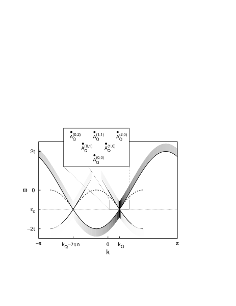
FIG. 2.: Schematic plot of the support of $A_{Q}(k,\omega)$ (above $\varepsilon_{c}$) and $B_{Q}(-k,\omega)$ (below $\varepsilon_{c}$) for $N/L=1/3$ and $Q=\pi/2$. The dominant tower ($p=0$) at $k=k_{Q}$ and the sub-dominant tower ($p=-1$) at $k=k_{Q}-2\pi n$ are shown. The weight mostly follows the solid lines, and the shadowing represent the intensity. Although there are excitations above the dashed line for $A_{Q}(k,\omega)$ as well, the weight associated with them is negligible. The low energy part of $A_{Q}(k,\omega)$ near $k=k_{Q}$ is enlarged on the insert, where the discrete states in the tower of excitations are shown.

FIG. 3.: $A_{Q}(\omega)$ for $Q=0$, $\pi/2$ and $\pi$ for quarter filling ($L=300$, $N=150$). For $Q=0$ the Van-Hove singularity is suppressed, and the weight is mainly near the Fermi energy. $Q=\pi$ is equivalent to free-fermion case. The dotted line shows the low-energy approximation Eq. (81).

FIG. 4.: $A_{Q}(k)$ for $Q=0$, $46\pi/91$($\approx\pi/2$) and $90\pi/91$($\approx\pi$) (a) and $B_{Q}(-k)$ for $Q=0$, $44\pi/89$($\approx\pi/2$) and $88\pi/89$($\approx\pi$) (b) for $L=270$ and $N=90$. The evolution of the weight and shape can be followed from the symmetric $Q=0$ case with the singularities at $k=0$ and $k=\pm 2\pi/3$ through the asymmetric $Q=\pi/2$ case with singularities at $k=\pi/6$ and $-\pi/2$ to the ‘normal’ distribution at $Q=\pi$.

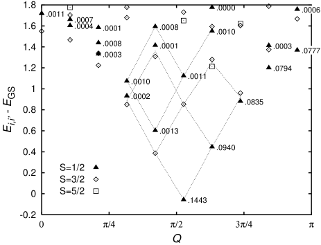
FIG. 5.: The support and weights of $C_{\sigma}(Q,\omega)$ for the $N=18$ spin Heisenberg model. The symbols represent the excitations of the final states (19 spins), where the total spin is also indicated. The numbers near solid triangles give the weight of that particular state. Due to selection rule the matrix elements are zero with higher spin states denoted by open symbols. The dotted lines are a guide to the eyes and show the $r=1/2$ and $r=-3/2$ towers.

FIG. 6.: The relative weights $c^{(1,0)}$, $c^{(2,0)}$, $d^{(0,1)}$ and $d^{(0,2)}$ as a function of the system size calculated by exact diagonalization (squares and triangles) and by DMRG (crosses) for the $r=1/2$ tower. The dashed line represents a fit to $a_{0}+a_{1}/N+a_{2}\log(N)/N$ form and it is reasonably close to the theoretical values $0.5$ and $0.375$ in the thermodynamic limit (a). The opposite sign of logarithmic corrections cancels if we make the products $[c^{(1,0)}d^{(0,1)}]^{1/2}$ and $[c^{(2,0)}d^{(0,2)}]^{1/2}$ (b).

FIG. 7.: $C_{\uparrow}(Q)$ and $D_{\uparrow}(Q)$ (a), $C_{\downarrow}(Q)$ and $D_{\downarrow}(Q)$ (b) for finite magnetization $N_{\uparrow}/N=3/4$ with singularity at $Q=3\pi/4$ and $Q=\pi/4$, respectively. The solid symbols stands for $D_{\sigma}(Q)$ and open for $C_{\sigma}(Q)$.