Conformations of Circular DNA

Abstract

We examine the conformations of a model for short closed DNA. The molecule is represented as a cylindrically symmetric elastic string with a constraint corresponding to a specification of the linking number. We obtain analytic expressions for configuration, elastic energy, twist and linking number for a family of solutions spanning from a circle to a ’figure eight’. We suggest ways to use our construction to make other configurations and models relevant to studies of DNA structure. We estimate the effect of thermodynamic fluctuations.

I introduction

The elastic model of DNA has been the subject of intense research in the past 30 years. The approaches taken include Lagrangian mechanics[1, 2, 3, 4, 5], b-splines and (numerical) molecular dynamics [6], and statistical mechanics[7]. Until now no one has been able to find the general equilibrium solutions for a bent twisted segment of the molecule. As a particular case the conformations of closed circular DNA have remained elusive.

In this paper we present a method for obtaining the shape, twist, elastic energy and linking number of an isotropic elastic segment subject to constraints. We will use this formalism to describe unknoted circular DNA. We will also outline how our formalism can be exploited to produce other shapes of interest to DNA researchers.

II Elastic Model and Expressions of Interest

In a previous work we outlined some developments in the elastic model of DNA[8]. The molecule is represented as a slender cylindrical elastic rod. At each point $s$ we describe the rod by relating the local coordinate frame ${\cal L}$ to the frame ${\cal L}_{0}$ rigidly embedded in the curve in its relaxed configuration. The relationship between the stressed and unstressed local frames is specified by Euler angles $\theta(s),\phi(s),\psi(s)$ needed to rotate ${\cal L}_{0}$ into $\cal L$. Let us summarize some of the results needed for this paper. Let the elastic constants of bending and torsional stiffness be denoted, respectively, by $A$ and $C$, and let $L$ be the lengh of the rod. The elastic energy is given by

$$E_{el}=\int_{0}^{L}ds\;\left(\frac{A}{2}\left(\dot{\phi}^{2}\sin^{2}\theta+\dot{\theta}^{2}\right)+\frac{C}{2}\left(\dot{\phi}\cos\theta+\dot{\psi}\right)^{2}\right)$$ (1)

The twist is

$${\cal T}w=\frac{1}{2\pi}\int_{0}^{L}ds\;\left(\dot{\phi}\cos\theta+\dot{\psi}\right)$$ (2)

A major relevant result from our previous work is that ${\cal L}k$, the linking number, can be written as

$${\cal L}k\;=\;-1\;+\;\frac{1}{2\pi}\int_{0}^{L}\left(\dot{\phi}+\dot{\psi}\right)\;ds\;\;$$ (3)

Where we have used Fuller’s theorem[9] to obtain the writhe, and White’s theorem[10] for the total link. We shall use these local quantities to determine the behaviour of the family of closed solutions that extremize the elastic energy.

III Candidates: The Elastic Extrema

A A Family of Curves

We are searching for a family of solutions which are extrema of elastic energy of a closed molecule. This family of ’writhing’ solutions will be indexed by the writhe, ${\cal W}r$, of a member - ranging from ${\cal W}r=0$ for a simple circle to ${\cal W}r=1$ for a ’figure eight’. We know that for ${\cal L}k\leq\sqrt{3}A/C$ the molecule remains stable as a circle [1, 12]. Therefore one bounding member of the family must be a simple circle, say, the $XY$ plane with a ${\cal T}w={\cal L}k=\sqrt{}3A/C$. We shall see that on the other end the bounding member, a ’figure eight’, must have ${\cal T}w=0$ in order to be an extremum of elastic energy. However, the reader must remember that the actual constraint imposed on the closed curve is that of a fixed ${\cal L}k$. We shall therefore examine the conditions under which the family of writhing curves can satisfy an imposition of a linking number constraint.

B Euler-Lagrange Minimization

We want to extremize elastic energy and keep the curve closed. We find that the functional to consider for closed configurations of DNA is

$${\cal H}=\int_{0}^{L}dE_{el}-F{\bf t}{\bf{\hat{z}}}\>ds$$ (4)

The first term of (4) is clear - the elastic energy must be extremized. The second term will enforce the closure in the ${\bf\hat{z}}$ direction only because we can always find a reference frame where the curve is closed in the $XY$ plane. Written explicitly as a function of Euler angles (4) becomes

$${\cal H}=\int_{0}^{L}\;ds\hskip 14.45377pt \frac{A}{2}\left(\dot{\phi}^{2}\sin^{2}\theta+\dot{\theta}^{2}\right)+$$ (5)

$$+ \frac{C}{2}\left(\dot{\phi}\cos\theta+\dot{\psi}\right)^{2}-F\cos\theta$$ (6)

The extrema are found by applying Euler-Lagrange equations to (6). Denoting the conserved quantities as $p_{\phi}\equiv\frac{\partial{\cal H}}{\partial\dot{\phi}}$ and $p_{\psi}\equiv\frac{\partial{\cal H}}{\partial\dot{\psi}}$ we get

$$\dot{\phi} = \frac{p_{\phi}-p_{\psi}\cos\theta}{A\sin\theta}$$ (7)

$$\dot{\psi} = \frac{p_{\psi}}{C}-\dot{\phi}\cos\theta$$ (8)

The equation for $\theta$ is a quadrature obtained by integrating $\frac{\partial{\cal H}}{\partial\theta}=\frac{d}{ds}\frac{\partial{\cal H}}{\partial\dot{\theta}}$ with $E_{0}$ as the constant of integration. Defining $u\equiv\cos\theta$ we see that the behavior of solutions is governed by a cubic polynomial in $u$:

$${\dot{u}}^{2} = \frac{2\left(1-u^{2}\right)}{A}\left(E_{0}-Fu\right)-\frac{1}{A^{2}}\left(p_{\phi}^{2}+p_{\psi}^{2}-2p_{\phi}p_{\psi}u\right)$$ (9)

$$\equiv \frac{2F}{A}\left(u-a\right)\left(u-b\right)\left(u-c\right)$$ (11)

$$\mbox{where we order the roots }c\leq u(\equiv\cos\theta)\leq b\leq a$$

(11) requires $\cos\theta$ to oscillate between $c$ and $b$. For a circular solution the tangent $\bf t$ will go back and forth twice.

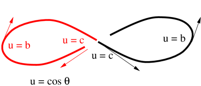
FIG. 1.: The tangent oscillates $c\rightarrow b\rightarrow c\rightarrow b\rightarrow c$. The curve is composed of two symmetric parts.

All the relevant quantities, including the shape of the curve, can be obtained using (11). For example:

$$\phi(s) = \int_{u(s=0)}^{u(s)}\frac{d\phi}{ds}\frac{ds}{du}du\;\;\;\mbox{ with }$$ (12)

$$\frac{ds}{du} = \sqrt{\frac{A}{2F}}\frac{1}{\sqrt{\left(u-a\right)\left(u-b\right)\left(u-c\right)}}$$ (13)

IV Constraints and Parameters

A Constraints

To complete the analysis we must determine the parameters generated by the minimization procedure: the invariants $p_{\phi}$ and $p_{\psi}$, the constant $E_{0}$, and the Lagrange multiplier $F$. To determine the parameters we impose constraints on the curve. Figure 1 is a good visual guide to the geometric meaning of the constraints that follow:

$$\int_{0}^{\frac{L}{2}}ds=L/2\;\;\;\; L$$ (fixing the length at ) (14)

$$\int_{0}^{\frac{L}{2}}u(s)ds=0\;\;\;\; z$$ (enforcing closure in ) (15)

$$\int_{0}^{\frac{L}{2}}\phi(s)ds=\pi\;\;\;\; \phi$$ ( must go all the way around) (16)

B Reparametrization

At this point we reparametrize the problem by $F,a,b,c$ instead of $F,E_{0},p_{\phi},p_{\psi}$. Parametrizing the problem by the roots of the polynomial is extremely advantageous: it makes the analytic manipulations more transparent; it also streamlines the computational tasks. The two sets of parameters are related in the following manner:

$$E_{0} = F\left(a+b+c\right))$$ (17)

$$p_{\phi} = \sqrt{\frac{AF}{2}}\left(p_{1}\pm p_{2}\right);\;\;\;p_{\psi}=\sqrt{\frac{AF}{2}}\left(p_{1}\mp p_{2}\right)$$ (18)

with $$\;p_{1\choose 2}\equiv\left[(c\pm 1)(b\pm 1)(a\pm 1)\right]^{1/2}$$ (19)

The choice of branch ($\pm$) is imposed by the family of configurations sought. For circular DNA without intrinsic curvature, $p_{\phi}$ takes a $-$, and $p_{\psi}$ correspondingly a $+$. Let us make some definitions that make notation more transparent:

$$\Delta b\equiv\left(b-c\right)\;\;;\;\;\Delta a\equiv\left(a-c\right)$$ (20)

$$q\equiv\sqrt{\frac{\Delta b}{\Delta a}}$$ (21)

Employing (13) we rewrite the constraint equations, (14), (15), and (16), in terms of the new parameters:

$$F=\frac{32A}{\Delta aL^{2}}K\left(q\right)\;\;\;\;$$ (22)

$$aK\left(q\right)=\Delta aE\left(q\right)$$ (23)

$$\pi/2\;\;=\;\;\frac{1}{\Delta a}\left[\left|\frac{(a+1)(b+1)}{(c+1)}\right|^{1/2}\Pi\left(\frac{\Delta b}{-1-c},q\right)\right.-$$ (24)

$$\hskip 61.17325pt-\left.\left|\frac{(a-1)(b-1)}{(c-1)}\right|^{1/2}\Pi\left(\frac{\Delta b}{1-c},q\right)\right]$$ (25)

Where $K,E\mbox{ and }\Pi$ are complete elliptic integrals of the first, second and third kind, respectively.

C Solving for $a$, $b$, $c$ and $F$

We find that the optimal procedure for calculation of solutions’ parameters is to use (22) to eliminate $F$, then (23) and (25) eliminate $\Delta a$ and $c$. Because the ${\cal W}r$ is a monotonically increasing function of $\Delta b$, we leave it to classify the family of curves. Once the constants $F,a,b,c$ are determined, the desired solutions and all the relevant quantities are computed via elliptic integrals. For example, the explicit expression for $\theta(s)$ in the first quarter of oscillation is (we have inverted (13)):

$$\cos\theta=\Delta b\mbox{ sn}^{2}\left(\sqrt{\frac{F\Delta c}{2A}}s,\sqrt{\frac{\Delta b}{\Delta a}}\right)-c$$ (26)

$\phi\mbox{ and }\psi$ are obtained similarly from (7) and (8).

The following figure shows the family of curves computed in the manner discussed above. Since the constraint equations involve elliptic integrals, finding a solution on a computer is virtually instanteneous.

FIG. 2.: The family of curves ranges from the circle in the $XY$ plane to the ’figure eight’ in the $YZ$ plane. The perspective is slightly assymetric to aid visualisation.

D Bounding Members: Circle and ’Figure Eight’

Let us check whether the initial member of our family, a circle with ${\cal W}r=0$ joins smoothly with the previously known stable family of twisted circles[11, 12]. The circle corresponds to ${\cal W}r=0$. A circle in the $XY$ plane the curve must have $b_{0}=c_{0}=0$. (25) now states that

$$\frac{1}{\sqrt{a}_{0}}\left(\sqrt{a_{0}+1}-\sqrt{a_{0}-1}\right)=1$$ (27)

which in turn gives (28)

$${p_{\psi}}_{0}=\frac{2\pi A}{L}\frac{1}{\sqrt{a}_{0}}\left(\sqrt{a_{0}+1}+\sqrt{a_{0}-1}\right)=\frac{2\pi A}{L}\sqrt{3}$$ (29)

Combining (2) and (8) to obtain the ${\cal T}w$ of the circle (29) gives

$${\cal T}w_{0}=\frac{L}{2\pi}{p_{\psi}}_{0}=\sqrt{3}\frac{A}{C}$$ (30)

It is also of interest to compute the ${\cal T}w$ of the ’figure eight’ which, like the circle, can be done virtually by inspection. The figure lies in the $YZ$ plane, which forces $\phi$ to behave as follows: (refer to Figure 1 for visualization)

$${\dot{\phi}}_{8}=\pi\left(\delta\left(0\right)+\delta\left(\frac{L}{2}\right)\right)$$ (31)

Combining (31) and (7) forces ${p_{\phi}}_{8}={p_{\psi}}_{8}=0$ which immediately sets ${\cal T}w_{8}=0$. The value of $\Delta b_{8}$ is easily determined from the fact that $c_{8}=-1$ (this can be seen from the curve itself) necessitating $a=1$. Then (25) gives $\Delta b_{8}=1.6522\ldots$.

V Linking Number and the Plectonemic Transition

We have found a family of writhing solutions that are the extrema of elastic energy. The writhe of the curves covers the range $0\leq{\cal W}r\leq 1$. However, the physical constraint imposed on the molecule is ${\cal L}k$, the linking number. The explicit expressions for ${\cal T}w$, ${\cal L}k$ and ${\cal W}r$ are easily obtained:

$${\cal T}w = \frac{2\pi}{\sqrt{\Delta a}}K\left(q\right)\left(p_{1}+p_{2}\right)\frac{A}{C}$$ (32)

$${\cal W}r = \frac{2\pi}{\sqrt{\Delta a}}\left[-K\left(q\right)\left(p_{1}+p_{2}\right)\right.$$ (33)

$$+ \left.\frac{p_{1}}{1+c}\Pi\left(\frac{\Delta b}{-1-c},q\right)+\frac{p_{2}}{1-c}\Pi\left(\frac{\Delta b}{1-c},q\right)\right]$$ (35)

and, using White’s theorem[10]

$${\cal L}k = {\cal T}w+{\cal W}r$$ (36)

Plotting ${\cal L}k$ vs. ${\cal W}r$ for our family we can discern three distinct types of behavior depending on the value of the ratio $A/C$.

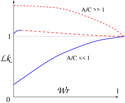
FIG. 3.: The three types of behaviour of ${\cal L}k$ for our writhing family of curves. The solid line indicates conformations realized by the molecule, whereas the dashed regions are forbidden by the imposition of ${\cal L}k$. The ratio $A/C$ controlls the plectonemic transition.

We can now describe what happens to the molecule as the linking number is increased. Initially the molecule remains a circle until $\Delta{\cal L}k=\sqrt{3}A/C$. After that there are three possibilities. If $A/C\ll 1$ then the writhing family can support a steady increase to ${\cal L}k=1$ of the ’figure eight’ and the molecule folds continuosly until self-crossing. (Futher increase of ${\cal L}k$ presumably results in a plectonemic configuration). If $A/C\gg 1$ then none of the members of the writhing family can support the neccesary linking number, and as soon as $\Delta{\cal L}k$ exceeds $\sqrt{3}A/C$ the twisted circle snaps into a plectoneme. An interesting case is the intermediate one, where, at first, the molecule starts writhing, but at some point, unable to support further increase in $\Delta{\cal L}k$ it snaps into a plectoneme. Another interesting fact is that this behavior is independent of the length of the molecule.

VI Possible Generalizations

A Intrinsic Curvature

The method of construction of the circular DNA can be easily generalized to other configurations of interest. Considerable activity has been generated around the studies of DNA with intrinsic curvature. We feel such generalizations are important because various chemical effects - hydrophobic, etc. - can be modeled by intrinsic curvature[13, 14, 15]. Inclusion of intrinsic curvature into the present framework involves a simple modification of the LHS of equation (25)[12]. If the inital curvature is such that the DNA is fully relaxed in the circular state, the characteristic polynomial (11) degenerates into a quadratic and all the quantities are expressible in terms of simple trigonometric functions. One complication does arise in cases of initial curvature: the solutions have to be minimized wrt to the initial value of $\psi$. An intuitive example of this caveat is the fact that the energy of intrinsically curved loops is changed by ’rolling’, unlike that of the configurations which are straight in their relaxed state.

B Trefoils and Other Torus Knots

Another interesting generalization of our results is obtained by altering the closure condition[12, 16]. For example, a curious configuration is attained by requiring the curve to close after $\phi$ has turned $4\pi\mbox{ rather than the }2\pi$ required for the closure of a circular conformation. The resulting curve is a trefoil knot. These curious shapes are probably the analytic analogs of similar configurations observed by Shlick and Olsen[6]. cite myself unpublished

VII Entropic Corrections

Although our model is applicable to the cases when thermodanamic fluctuations are not important (i.e. short segments) it is worth while to estimate the contribution of thermal fluctuations to the free energy. Since the aim of this paper is to derive the elastic shapes of DNA, we will concentrate on thermal effects that influence curvature. This can be done in analogy to Marko and Siggia [17] who, in turn, used the scaling ideas originally developed for the study of fluctuating membranes[18]. Their (slightly generalized) dimensional analysis states that the entropic contribution to the free energy can be written as

$${\Delta f} = k_{B}T\>\left(\frac{\kappa^{2}}{A/k_{B}T}\right)^{1/3}$$ (38)

where the curvature $$\kappa$$ is

$$\kappa^{2} = \dot{\theta}^{2}+\dot{\phi}^{2}\sin\theta^{2}$$ (39)

We conceed that equation (38) gives only the form of the thermal correction, sans the multiplicative factor of order unity. (38) reflects the fact that increasing the curvature reduces the correlation length, thus suppressing fluctuation and incurring a corresponding loss of entropy.

VIII Conclusion

We have presented a formalism for obtaining the elastic mimima of circular DNA subject to a constraint in the linking number. Aside from the simplicity of the statement of the problem, and the beauty (in the eyes of the creators) of the solution, our formalism can significantly improve the investigations of linear molecules with elastic models. This method can be easily generalized to create a truly ’finite’ finite-element-analysis in which elastic models can be traced out by finite segments. The conformations of these segments can be specified in close form which would decrease computation time significantly.

REFERENCES

- [1] Benham C.J. Biopolymers 22, 2477-2495 (1983).
- [2] Le Bret M. Biopolymers 23, 1835-1867 (1984).
- [3] Tsuru H. and Wadati M. Biopolymers 25 2083-2096 (1986).
- [4] Tanaka F. and Takahashi H. J. Chem. Phys. 83(11) 6017-6026 (1985).
- [5] Manning R.S., Maddocks J.H., Kahn J.D. J. Chem. Phys. (submitted) (1996).
- [6] Schlick T. and Olsen W. Science 257, 1110-1115 (1992).
- [7] Marko J.F. and Siggia E.D. Phys. Rev. E 52, 2912-2938 (1995).
- [8] Fain B., Rudnick J., Östlund S. Phys. Rev. E (to be published) (1997).
- [9] Fuller F.B. Proc. Natl. Acad. Sci. USA No.8, 3357-3561 (1978).
- [10] White J.H. Am. J. Math. 91 No.3, 693-727 (1969).
- [11] Benham C.J. Phys. Rev. A 39 2582-2586 (1988)
- [12] B. Fain, unpublished.
- [13] Boles T.C., White J.H. and Cozzarelli N.R. J. Mol. Biol. 213, 931-951 (1990).
- [14] Bauer W.R., Lund R.A., White J.H. Biochemistry v. 90 833-837, (1992).
- [15] Tobias I., Olsen W.K., Biopolymers v. 33 639-646, (1993).
- [16] Nussinov Z., private communication.
- [17] Marco J.F. and Siggia E.D. Science 265 506-508, (1994).
- [18] Safran S.A., Stat. Phys. of Surfaces, Interfaces, and Membranes, ch. 6.5, Addison Wesley (1994).