[

Phase diagram of glassy systems in an external field

Abstract

We study the mean-field phase diagram of glassy systems in a field pointing in the direction of a metastable state. We find competition among a “magnetized” and a “disordered” phase, that are separated by a coexistence line as in ordinary first order phase transitions. The coexistence line terminates in a critical point, which in principle can be observed in numerical simulations of glassy models.

]

The crossover from supercooled liquids to glasses, although manifestly an off-equilibrium phenomenon, presents characteristics reminiscent of equilibrium phase transitions [2]. Probed at fixed observation time scale, the various thermodynamic quantities show non-analytic behavior at the glassy temperature $T_{g}$. While the singularity is pushed to lower temperatures for increasing observation times, it does not seen to decrease in intensity. Whether for infinite probing times the singularity persists to produce a “true” finite temperature phase transition is a longly debated question, and is at present experimentally and theoretically unsolved. Experimentally, due to the rapid growth of the relaxation time as temperature is lowered, it is difficult to equilibrate the systems at temperatures that exceed the estimated critical temperature by less then 15 %. Theoretically, the only well established issues rely on mean-field approximation. Mean field theory for disordered models that are conjectured to be in the same universality class of structural glasses, predicts a thermodynamical transition, along the Gibbs-DiMarzio scenario of the entropy crisis at finite temperature $T_{s}$ [3]. The transition at $T_{s}$ combines features of first order and second order phase transitions. Like in a second order phase transition the energy is continuous and the specific heat has a jump. Like in a first order phase transition there is no divergent susceptibility. Detailed studies of the mentioned models [3] have shown that it exists an interval of temperatures $T_{s}<T<T_{d}$ where the thermodynamic, as well as the dynamic is dominated by the existence metastable states, which can trap the system for infinite time. In finite dimension the picture must necessarily be modified, as metastable states can not have a infinite time life. An appealing possibility is that metastable states continue to exist with finite decay time. Transitions among metastable states would dominate the dynamics in that region. The inclusion of these phenomena is one of the most challenging problem in the theory of glasses [4].

In ordinary mean-field theories the appearance of metastable states is signaled by local minima of the “potential function”, the free-energy as a function of the order parameter, and can be stabilized by the introduction of an external field coupled with the order parameter. In glasses, while the system is dynamically frozen, long range order is absent and it is impossible to identify any intrinsic (physical) order parameter for a single system allowing to distinguish different thermodynamical states. The usual Edwards-Anderson parameter, that measure the degree of freezing, takes the same value in all the dominant states. Spin glass theory [5] suggests that measures of distance (or alternatively similarity) among different “real replicas” can be taken as appropriate order parameter. A potential, or better a class of potential functions, can be defined considering the partition function of several real replicas with constraints on the mutual distances [6]. Alternatively one can release the constraints and introduce a field coupled to the distances. The two constructions are related by the Legendre transform, and both have been employed to study glassy systems [6, 7, 8, 9]. This point of view, although it can not help in real experiments, can give theoretical insights, and can be useful in numerical experiments. Different question can be addressed with different potential function. In this paper we limit ourselves to potentials involving two real replicas. More complicated three-replica potential have been considered in [10, 11]. Let us, to be defined, consider a system of $N$ interacting variables $S_{i}$, $i=1,...,N$, with Hamiltonian $H({\bf S})$, and be $q({\bf S},{\bf S}^{\prime})$ an overlap function, i.e. an intensive measure of similarity among the configurations ${\bf S}$ and ${\bf S}^{\prime}$. We can consider two replicas of the system trying to thermalize at the same temperature with an attractive coupling. The appropriate thermodynamical description of this situation is given by the partition sum:

$$Z_{A}=\sum_{{\bf S}_{1},{\bf S}_{2}}\exp\left[-\beta(H({\bf S}_{1})+H({\bf S}_{2}))+\beta\epsilon Nq({\bf S},{\bf S}^{\prime})\right].$$ (1)

We will call $\Gamma_{A}(\epsilon)=-T/N\log Z_{A}$ the annealed potential. Alternatively, we can consider a reference configuration ${\bf\sigma}$ thermalized at temperature $T^{\prime}$, acting as an external field on a replica ${\bf S}$ which tries to thermalize at temperature $T$. In this case the right partition function is

$$Z_{Q}=\sum_{{\bf S}}\exp\left[-\beta H({\bf S})+\beta\epsilon Nq({\bf S},{\bf\sigma})\right],$$ (2)

and $\Gamma_{Q}(\epsilon)=-T/N\log Z_{Q}$ will be the quenched potential. The idea of the quenched potential is particularly appealing for the physics of glasses. At a given cooling rate, the system equilibrates within the super-cooled liquid phase, until the glassy transition temperature $T_{g}$ is reached. Below that temperature it is reasonable to think that the system will be stacked for a long time in a metastable state. While fast degree of freedom thermalize at temperature $T$, the slow degree of freedom will remain confined for a long time close to the equilibrium configuration reached at $T_{g}$. In such conditions, restricted Boltzmann-Gibbs averages generated by a partition function of the kind (2) with $T^{\prime}$ identified with $T_{g}$ could be appropriate. In this pseudo-thermodynamic description the parameter $\epsilon$, which fixes the equilibrium value of the overlap with the reference configuration, should be considered as a dynamical variable, fixed by the condition that the system has equilibrated in the neighbors of the reference configuration ${\bf\sigma}$, but has not had the time necessary to escape from the metastable state. Within the limit of validity of this picture the usual laws of thermodynamics must hold in the glassy phase. The picture certainly loose its validity for times large enough to escape from the metastable state and aging dynamics sets in the system [12].

The quenched case in an infinitesimal field and $T=T^{\prime}$ was studied in detail in [8]. In this paper we extend the analysis to the equilibrium phase diagram of the quenched potential in the $T-\epsilon$ plane. For definiteness let us introduce the model that we will use in the following, the same lines of reasoning can be followed in general. The model we study is a spherical $p$-spin model [13]. This is defined in terms of $N$ real dynamical variables $S_{i}$, ($i=1,...,N$) subjected to the constraint $\sum_{i=1}^{N}S_{i}^{2}=N$ and interacting via a random Gaussian Hamiltonian $H({\bf S})$, defined by its correlator $\overline{H({\bf S})\;H({\bf S}^{\prime})}=Nf(q_{{\bf S},{\bf S}^{\prime}})$. The overlap $q_{{\bf S},{\bf S}^{\prime}}$ is a measure of similarity among configurations and is given by $q_{{\bf S},{\bf S}^{\prime}}=1/N\sum_{i}S_{i}S_{i}^{\prime}$. If the correlation function is taken of the monomial form $f(q)=1/2q^{p}$ the Hamiltonian can be represented as $H=-\sum_{i_{1}<...<i_{p}}^{1,N}J_{i_{1},...,i_{p}}S_{i_{1}}...S_{i_{p}}$ with independent centered Gaussian couplings $J_{i_{1},...,i_{p}}$, which motivates the name of the model. We will stick to this case throughout all this paper. The model has been studied extensively during the last years, and furnishes, for $p>2$, a good mean-field model of fragile glass. It has been often observed [3] that the Langevin relaxation of this model leads to equations homologous to those of mode coupling theory [14].

The quenched free energy $\Gamma_{Q}[{\bf{\bf\sigma}};\beta,\epsilon]$ should be self-averaging with respect to the distribution of ${\bf\sigma}$, so we can compute it as $\Gamma(\epsilon,T,T^{\prime})=-1/Z\sum_{{\bf\sigma}}\exp(-\beta^{\prime}H({\bf\sigma}))T/N\log Z[{\bf{\bf\sigma}};\epsilon]$. In the following we will study the phase diagram of the model in the $\epsilon-T$ plane in two situations: a) $T^{\prime}=T$, corresponding to restricting the partition sum to the vicinity of a particular equilibrium state at each temperature. b) $T^{\prime}$ fixed, corresponding to probe the evolution of the free-energy landscape in the vicinity of a fixed configuration of equilibrium at $T^{\prime}$ when $T$ is changed.

The Legendre transform of $\Gamma(\epsilon,T,T^{\prime})$, $V(q,T,T^{\prime})\equiv\min_{\epsilon}\Gamma(\epsilon)+\epsilon q$, which corresponds physically to constraining the value of $q_{{\bf S},{\bf\sigma}}$ to $q$, was studied in detail in [9] with the aid of the replica method. The interested reader can found there details about the general method and the analytic expression for $V$ in the case of the spherical $p$-spin model.

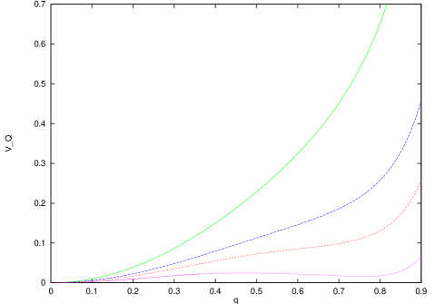
FIG. 1.: The potential as a function of $q$ for $T^{\prime}=2T_{s}T_{d}/(T_{s}+T_{d})$ and various values of $T$, in order of decreasing temperatures from top to bottom.

The shape of the function $V$ turned out to be the characteristic one of a mean-field system undergoing a first order phase transition. At high enough temperature $V$ is an increasing and convex function of $q$ with a single minimum for $q=0$. Decreasing the temperature to a value $T_{f}$, where for the first time a point $q_{f}$ with $V^{\prime\prime}(q_{f})=0$ appears, the potential looses the convexity property and a phase transition can be induced by a field. A secondary minimum develops at $T_{d}$, the temperature of dynamical transition [3], signaling the presence of long-life metastable states. The minimum of the potential has received a dynamical interpretation [9, 15] as corresponding to the states reached at long times by the evolution at temperature $T$ starting at time zero from an equilibrium configuration at temperature $T^{\prime}$. This allows to fix $q$ in the pseudo-thermodynamical description mentioned above to the value it takes in the minimum of the potential. The height of the secondary minimum reaches the one of the primary minimum at $T=T_{s}$ and coexistence in zero field takes place. This is the usual statical transition point in zero field, and it is not accompanied by the release of latent heat. In figure 1 we show the shape of the potential in the various regions. The attentive reader would have noticed that respect to the curves presented in [9] only one secondary minimum is present at low temperature. The results we present here are corrected taking into account replica symmetry breaking effects, the meaning of which will be discussed in [16]. Although the behavior of the potential function is analogous to the one found in ordinary systems undergoing a first order phase transition the interpretation is here radically different. While in ordinary cases different minima represent qualitatively different thermodynamical states (e.g. gas and liquid), this is not the case in the potential discussed here. In our problem the local minimum appears when ergodicity is broken, and the configuration space splits into an exponentially large number of components. The two minima are different manifestations of states with the same characteristics. The height of the secondary minimum, relative to the one at $q=0$ measures the free-energy loss to keep the system in the same component of the quenched one. At equal temperatures $T=T^{\prime}$ this is just the complexity $T\Sigma$, i.e. the logarithm of the number of distinct pure states of the system. For $T\neq T^{\prime}$ it also takes into account the free-energy variation of the equilibrium state at temperature $T^{\prime}$ when followed at temperature $T$.

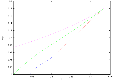
FIG. 2.: Phase diagram in the $\epsilon-T$ plane for $T^{\prime}=T$. The upper curve is the spinodal of the disordered state, the lower one the spinodal of the magnetized state, and the middle curve the coexistence line. The coexistence line touches the axes $\epsilon=0$ at $T=T_{s}$, while the spinodal of the magnetized state touches it at $T=T-d$. For $T<T_{s}$ the spinodal of the disordered state remains finite and touches the $T=0$ axes at finite $\epsilon$.

The presence of the field $\epsilon$ adds finite stability to the metastable state, and the transition is displaced at higher temperatures. In figure 2 we display the phase diagram of the $p=4$ model in the case $T^{\prime}=T$. The coexistence line departs from the axes $\epsilon=0$ at the transition temperature $T_{s}$ and reaches monotonically a critical point $(T_{cr},\epsilon_{cr})$. In figure 2 it is also shown the spinodal of the “magnetized” solution, which touches the $\epsilon=0$ axes at the dynamical temperature $T_{d}$, and the spinodal of the “disordered” solution for temperaratures larger then $T_{s}$.

The coexistence line for $T^{\prime}$ fixed in the interval $T_{d}\leq T^{\prime}\leq T_{s}$ is qualitatively similar to the one of figure 2 at high enough temperature, but (for $T^{\prime}>T_{s}$) it never touches the axes $\epsilon=0$.

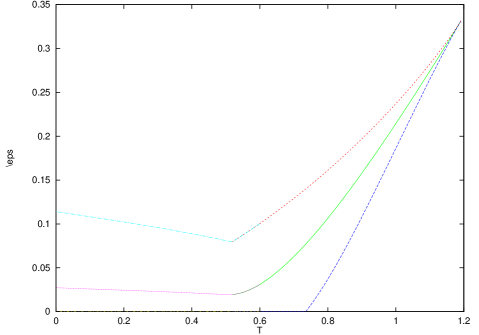
FIG. 3.: Phase diagram in the $\epsilon-T$ plane for $T^{\prime}=2T_{s}T_{d}/(T_{s}+T_{d})$. The upper curve is the spinodal of the disordered state, the lower one the spinodal of the magnetized state, and the middle curve the coexistence line.

Even at zero temperature there is a first order phase transition in $\epsilon$, reflecting the fact that the ground state of the system is lower then the energy of the reference state when followed at $T=0$. This can be seen in figure 3 where we show the phase diagram for $T^{\prime}=2T_{s}T_{d}/(T_{s}+T_{d})$. At the critical point the transition is second order.

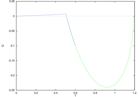
FIG. 4.: Latent heat of the transition as a function of the temperature for $T^{\prime}$ as in fig. 3.

While the transition in zero field is not accompanied by heat release, a latent heat is present in non zero $\epsilon$. In figure 4 we show, in the same conditions of fig. 3, the latent heat ${\cal Q}=E_{+}-E_{-}-\epsilon(q_{+}-q_{-})$ where $E_{+}$ ($q_{+}$) and $E_{-}$ ($q_{-}$) are the internal energies (overlaps) respectively of the magnetized and unmagnetized states. Notice that (as it should) the latent heat is zero at the critical point and at $T=0$. The magnetized state roughly reflects the properties of the equilibrium states at temperature $T^{\prime}$ followed at temperature $T$, while the disordered state reflects the properties of the true equilibrium states at temperature $T$. We see that at high temperature the magnetized state is energetically favored, while at low temperature it has an energy higher then the one of equilibrium. The point where ${\cal Q}$ changes sign does not correspond to a second order phase transition. Finally, in figure 5 we show, for a fixed temperature the curve of $q(\epsilon)$ obtained by the Maxwell construction.

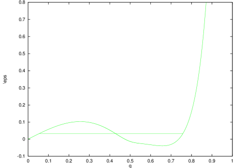
FIG. 5.: Equation of state for $T^{\prime}=2T_{s}T_{d}/(T_{s}+T_{d})$ and $T=0.609$. The horizontal line corresponds to coexistence and is obtained by the Maxwell construction.

So far we have presented results for the quenched potential $\Gamma_{Q}$. In the annealed case, it was shown in [7] the potential $V_{a}$ has qualitatively the same shape than the quenched one ($V_{Q}$); it can therefore be expected a phase diagram similar to the one of figure 2 also in this case.

Although we have based our discussion on a mean-field model, we expect that the qualitative features of the phase diagrams presented survive in finite dimension. We belove that the existence of a coexistence line, terminating in a critical point, is a constitutive feature of systems whose physics is dominated by the existence of long lived metastable states. The predictions of this paper can be submitted to numerical test in glassy model systems as like e.g. Lennard-Jones or hard spheres, or polymer glasses. For example the identification of the complexity $\Sigma$ as the free energy difference between the stable and the metastable phases allows a direct measure of this quantity in a simulation. Indeed the ending of the transition lines in a critical point implies that the metastable state can be reached via closed paths in phase diagram leaving always the system in (stable or metastable) equilibrium; and the free energy difference of the two phases computed integrating the specific heat a long the loop.

Acknowledgments

The authors benefited of the stimulating environments of the conferences of Sitges (10 - 14 June 1996) and Lyon (30 September - 3 October 1996). SF thanks the “Dipartimento di Fisica dell’ Università di Roma La Sapienza” for kind hospitality during the elaboration of this work.

REFERENCES

- [1]
- [2] For review see, W. Gotze, Liquid, freezing and the Glass transition, Les Houches (1989), J. P. Hansen, D. Levesque, J. Zinn-Justin editors, North Holland; C. A. Angell, Science, 267, 1924 (1995)
- [3] T. R. Kirkpatrick and D. Thirumalai, Phys. Rev. B36 (1987) 5388 ; T. R. Kirkpatrick and P. G. Wolynes, Phys. Rev. B36 (1987) 8552; a review of the results of these authors and further references can be found in T. R. Kirkpatrick and D. Thirumalai Transp. Theor. Stat. Phys. 24 (1995) 927.
- [4] G. Parisi, preprint cond-mat 9411115, 9412004, 9412034
- [5] M. Mézard, G. Parisi and M. A. Virasoro, Spin Glass Theory and Beyond (World Scientific, Singapore 1987);
- [6] S. Franz, G. Parisi, M. A. Virasoro, J.Physique I 2 (1992) 1969,
- [7] J. Kurchan, G. Parisi, M. A. Virasoro, J.Physique I 3 (1993) 1819
- [8] R. Monasson, Phys. Rev. Lett. 75 (1995) 2847
- [9] S. Franz, G. Parisi, J. Physique I 5 (1995) 1401
- [10] S. Franz, G. Parisi, M. A. Virasoro, Europhys.Lett. 22 (1993) 405
- [11] A. Cavagna, I. Giardina, G. Parisi preprint cond-mat/9611068
- [12] L. C. E. Struik; Physical aging in amorphous polymers and other materials (Elsevier, Houston 1978).
- [13] T. R. Kirkpatrick, D. Thirumalai, Phys. Rev. B36, (1987) 5388; A. Crisanti, H. J. Sommers, Z. Phys. B 87 (1992) 341. A. Crisanti, H. Horner and H. J. Sommers, Z. Phys. B92 (1993) 257. L. F. Cugliandolo and J. Kurchan, Phys.Rev.Lett.71 (1993) 173;
- [14] E. Leutheusser, Phys. Rev.A29, 2765 (1984); T. R. Kirkpatrick, Phys. Rev A31, 939 (1985); W. Gotze and L. Sjogren, Rep. Prog. Phys. 55, 241 (1992)
- [15] A. Barrat, R. Burioni and M. Mezard, Preprint cond-mat 9509142
- [16] A. Barrat, S. Franz, G. Parisi, in preparation.