NUMERICAL SIMULATIONS OF SPIN GLASS SYSTEMS

We discuss the status of Monte Carlo simulations of (mainly finite dimensional) spin glass systems. After a short historical note and a brief theoretical introduction we start by discussing the (crucial) $3D$ case: the warm phase, the critical point and the cold phase, the ultrametric structure and the out of equilibrium dynamics. With the same style we discuss the cases of $4D$ and $2D$. In a few appendices we give some details about the definition of states and about the tempering Monte Carlo approach.

1 Introduction

Spin glasses are a fascinating subject, both from the experimental and from the theoretical point of view $\!{}^{{\bf?},{\bf?},{\bf?},{\bf?}}$. In the framework of the mean field approximation a deep and complex theoretical analysis is needed to study the infinite range version of the model (the Sherrington-Kirkpatrick model, SK model in the following). Using the formalism of replica symmetry breaking $\!{}^{{\bf?}}$ (RSB) one finds an infinite number of pure equilibrium states, which are organized in an ultrametric tree. It is fair to say that while most of the equilibrium properties of the SK model are well understood, much less is known about the detailed features of the dynamics, although recent progresses have been done in this direction.

A crucial question is how much of this very interesting structure survives in short range models, defined in finite dimensional space. Numerical simulations are very useful for trying to answer this question, since most of the more peculiar predictions are for quantities that is difficult to relate to measurements that can be performed in real experiments.

Our goal will eventually be to draw a meaningful comparison of the theoretical findings and the experimental data. In order to do that we will discuss the mean field picture that we have introduced before and a different point of view, the droplet model $\!{}^{{\bf?},{\bf?},{\bf?}}$. We will see that a comparison of the predictions of the mean field theory with those arising from the droplet model systematically shows the appropriateness of the mean field picture.

In the most part of cases an interacting theory is formulated by starting from a limiting case which is well under control. Then one constructs some kind of perturbation expansion, but the features one finds in this way typically share many features with the starting point one used: one better starts from a good guess. In spin glasses there are two different starting point that have been considered in the literature:

• The mean field approximation, which is correct in the infinite dimensional limit.

• The Migdal-Kadanoff (MK) approximation $\!{}^{{\bf?}}$, which is (trivially) correct in one dimension and for some fractal lattices (e.g. carpet lattices). This approximation is the basis of the so called droplet model (hereafter DM).

It is known that the MK approximation gives results that are violently wrong from a quantitative point of view when we go to a large dimensionality space (in most models the results are acceptable only in dimension $2$ or less). For example in a ferromagnet the MK approach does not detect the triviality of the critical exponents in dimensions greater than $4$. Usually the MK approximation grasps correctly the qualitative behavior (e.g. the existence of Goldstone modes in models with spontaneously broken $O(N)$ symmetry) in the low temperature phase and from this point of view it agrees with the mean field predictions.

There is no controversy on the behavior at the transition point in spin glasses is concerned in zero external magnetic field. Critical exponents are given by the mean field in more than six dimension and a (poorly convergent) $\epsilon$-expansion predicts the exponents in $6-\epsilon$ dimensions $\!{}^{{\bf?},{\bf?}}$.

On the contrary in the low temperature phase the two approaches imply a very different behavior. Mean field theory predicts that for a large, finite system , there are many different equilibrium states. The droplet approach predicts that the equilibrium state is unique, apart from reflections. The two points of view drastically differs in the properties of overlap: in the droplet model the value of the overlap $q$ among two different real replicas of the systems is expected to be a given number, while in the mean field approach it has a non trivial probability distribution $P(q)$, which in the infinite volume limit has support in the interval $(q_{m},q_{M})$ ($q_{m}$ stands for the minimum $q$ value, $q_{M}$ stand for the maximum $q$ value). The value $q_{M}$ coincides with the overlap among two generic configurations in the same state, which is denoted $q_{\rm EA}$ ($\rm EA$ stands here for Edwards-Anderson). The probability distribution for a given sample $P_{J}(q)$ is a quantity that depends on the sample: it is a non self-averaging quantity.

This difference in the expectations for $q$ has strong implications for the magnetic susceptibility: in the droplet model in the limit of zero magnetic field there is no ambiguity in the definition of the susceptibility and it is given by the relation

$$\chi=\beta(1-q_{\rm EA})\ .$$ (1)

In the mean field approach there are two different susceptibilities:

• The linear response susceptibility ($\chi_{LR}$) which is given by the zero frequency limit of the time dependent susceptibility (equivalently it is given by variation of the magnetization when an infinitesimal magnetic field is applied to a system in a pure state). It is given by:

  $$\chi_{LR}=\beta(1-q_{\rm EA})\ .$$ (2)

• The equilibrium susceptibility, i.e. the derivative of the equilibrium magnetization with respect to the magnetic field. It is given by the relation:

  $$\chi_{eq}=\beta\int{\rm d}q~{}(1-q)P(q)\geq\chi_{LR}\ .$$ (3)

  With very good approximation $\chi_{eq}$ is given experimemtally by the derivative of the thermoremanent magnetization with respect to the magnetic field.

In the droplet model the two suscetibilities are equal. In the mean field approach we have $\chi_{LR}<\chi_{eq}$ in the broken phase, while in the warm phase $q_{\rm EA}=0$ and we get that both susceptibilities are given $\beta$. In the broken phase region we have $\chi_{eq}>\beta(1-q_{\rm EA})$.

The difference of the two susceptibilities is a typical prediction of the mean field theory; indeed in the first case ($\chi_{LR}$) the system in presence of an infinitesimal magnetic field must be very similar from that in zero magnetic field. In the second case systems at equilibrium in different magnetic fields may correspond do very different microscopical configurations.

In many cases numerical simulations have been extremely useful to discriminate among different theoretical scenarios and to discover the existence of possible non perturbative effects. Spin glasses are not an exception to this rule, although numerical simulations are much more difficult here than in the usual ferromagnetic case $\!{}^{{\bf?}}$. The main difficulty is related to the high value of the dynamic exponent $z$. Already in mean field $z$ is quite large ($4$) and it becomes still larger in three dimensions (around $6$). This is very different from usual ferromagnets, where $z$ has a small value (close to $2$), largely independent from the system dimensionality.

Most of the numerical simulations have been ran in three dimensions, where it is more difficult to get satisfactory results (we will discuss this issue in much detail in the following). The situation in two and four dimension has been clarified by numerical simulations (for opposite reasons: see later) in a far more complete and satisfactory way. Although the behavior of finite dimensional spin glass systems in presence of a magnetic field is very interesting unfortunately only few data are available.

In section (2) we use a few phrases to describe the earlier generation series of Monte Carlo simulation: we will not have space to describe them in detail, and we will just draw the main findings. In section (3) we define the models, and give the definitions we will use in the text. In section (4) we give a mini-theoretical review. We start the bulk of our discussion by the crucial case of $3$ dimensions (5): we discuss simulations in the high $T$ phase (5.1), in the broken phase (5.2), simulations using three replicas of the system (5.3) and off-equilibrium dynamic simulations (5.4). We discuss how the existence of a phase transition has been made clear, and how one qualifies the broken phase, showing it is broken according to the mean field RSB pattern. After that we discuss the case of $4D$ (6), where the existence of a mean field like broken phase it is absolutely clear from the numerical point of view. The case of $2D$ , where one does not have a finite $T$ phase transition, is discussed in (7) to stress peculiar effects and behaviors of interest. In a series of appendices we discuss about pure state (Appendix 1: On the Definition of Pure States.), and about improved Monte Carlo Methods (tempering (Appendix 2: Simulated Tempering) and parallel tempering (Appendix 3: Parallel Tempering)).

We realize that there are many very interesting subject that we have not considered for lack of space: we only quote the numerical simulations in Hamiltonian infinite range models with Ising, Heisenberg or spherical spins with interactions connecting two or more spins$\!{}^{{\bf?},{\bf?},{\bf?}}$; the whole series of questions connected to non-Hamiltonian system $\!{}^{{\bf?}}$; non-Ising spins in finite dimensions $\!{}^{{\bf?}}$; Ising spin glass at the upper critical dimension $\!{}^{{\bf?}}$; chaos in spin glasses $\!{}^{{\bf?}}$ and quantum spin glasses $\!{}^{{\bf?}}$. There is surely much more that we are omitting, and we apologize.

2 History

The papers by Ogielski and Morgenstern $\!{}^{{\bf?}}$ and by Bhatt and Young $\!{}^{{\bf?}}$ start somehow the history of modern, large scale simulations of finite dimensional spin glass models. They both deal with $3D$ systems, with quenched random couplings $J=\pm 1$ with probability $\frac{1}{2}$. A special purpose computer has been built for running the simulations of $\!{}^{{\bf?}}$: this has been one of the milestones of the history of computers dedicated or optimized (as far as the hardware is concerned) for the study of problems in theoretical physics.

Ref. $\!{}^{{\bf?}}$ deals with both equilibrium and dynamics. The best output of the simulations is that there is a phase transition at $T_{c}=1.20\pm 0.05$, with $\nu=1.2\pm 0.1$, but if a $T=0$ power law divergence can be excluded an exponential divergence of the kind $\xi\simeq\exp(b/T^{c})$ (that is what we expect at the lower critical dimension, LCD, see later) fits very well the data. The dynamic simulations allow to estimate a correlation time that assuming a phase transition scales like $\tau(T)\simeq\xi^{z}$, with $z\simeq 5$. An exponential fit to a LCD form works fine. Also a Vogel-Fulcher behavior $\tau\simeq\tau_{0}\exp(\frac{\Delta F}{T-T_{0}})$ with $T_{0}\simeq 0.9$ fits well the data.

If one assumes the existence of a phase transition the work of $\!{}^{{\bf?}}$ gives compatible results, with $T_{c}\simeq 1.2$, $\nu=1.3\pm 0.3$ and $\eta=-0.3\pm 0.2$, but the simulations at not so high $T$ values make the possible LCD behavior very clear. The spin glass susceptibility $\chi_{q}$ is estimated here with two different approaches (two copies of the system or dynamic correlation functions). The two possibilities of $3$ being the LCD and of a Kosterlitz-Thouless like transition are compatible with the data.

In a longer paper Ogielski $\!{}^{{\bf?}}$ mainly discusses the dynamic behavior of the $3D$ system. He finds that for $T>T_{c}$ the dynamic correlation functions can be described by a stretched exponential decay, while in the cold phase one always detects power law (a typical signature of the slow dynamics of a complex system). The dynamic exponent $z$ turns out to be close to $6$. Again, one gets hints for dimension $3$ being marginal or close to it. The dynamic behavior of the $3D$ model has also been studied by Sourlas $\!{}^{{\bf?}}$, while looking at domain walls gives compatible results $\!{}^{{\bf?}}$.

Bhatt and Young $\!{}^{{\bf?}}$ study the cases $2D$, $3D$ and $4D$, with a systematic analysis of the Binder parameter $g$ (and an accurate study of thermalization). In $2D$, with $J=\pm 1$ (here there can be a difference from the case of continuous couplings, since the ground state has an accidental degeneracy: $\eta$ for example is not expected to be universal) $T_{c}=0$. Assuming a power divergence gives $\nu=2.6\pm 0.4$, $\eta=.20\pm.05$ and $\gamma=4.6\pm 0.5$. In $3D$ they study the case of Gaussian couplings, to investigate universality. Again one finds that the existence of a phase transition is favored, but the LCD is very close. $4D$ appears as an easy case. The critical region is clear, and one can easily get a rough but reliable estimate $\nu=0.80\pm 0.15$, $\eta=-.30\pm.15$ and $\gamma=1.8\pm 0.4$.

Ergodicity breaking in $3D$ has been discussed by Sourlas in $\!{}^{{\bf?}}$.

The work by Reger, Bhatt and Young $\!{}^{{\bf?}}$ uses the observation that $4D$ is a simple case to make it a test case. Ref. $\!{}^{{\bf?}}$ clearly shows that the broken phase of the $4D$ system has a non-trivial overlap probability distribution: things go exactly as they do in the mean field model. After ref. $\!{}^{{\bf?}}$ one has to turn a triple somersault in order to claim that the mean field limit is not a good starting point to study the realistic case of finite $D$ dimensional models, with $D$ lower than the upper critical dimension and higher than the lower one.

3 Definitions

We give here some definitions that will be needed in the following. We work in $D$ spatial dimensions. The linear extension of our lattice is $L$, and the volume is $V=L^{D}$ (sometimes we will denote it with $N$). In the mean field model $N$ or $V$ denote the total number of lattice sites. Typically we work with Ising spins $\sigma_{i}=\pm 1$. The Hamiltonian is

$$H\equiv\sum_{<i,j>}\sigma_{i}J_{i,j}\sigma_{j}\ ,$$ (4)

where the sum runs over first neighbor on the $D$ dimension (simple cubic, where we do not specify something different) lattice, and the $J$ are quenched random variables. The couplings $J$ will be sometimes Gaussian, and sometimes they will take the value $\pm 1$ with probability $\frac{1}{2}$ (see text). The magnetization is

$$m\equiv\frac{1}{V}\sum_{i}\sigma_{i}\ .$$ (5)

In spin glasses it is not a very interesting quantity, since by using the gauge invariance of the theory one can show that $\overline{\langle m\rangle}=0$. The magnetic susceptibility is

$$\chi\equiv\frac{1}{V}\overline{\langle m^{2}\rangle}\ .$$ (6)

The overlap among two configurations $\alpha$ and $\beta$ at site $i$is

$$q_{i}^{\alpha,\beta}\equiv\sigma_{i}^{\alpha}\sigma_{i}^{\beta}\ ,$$ (7)

and the total overlap

$$q^{\alpha,\beta}\equiv\frac{1}{V}\sum_{i}q_{i}^{\alpha,\beta}\ ,$$ (8)

where we will frequently ignore the superscripts by denoting it with $q$. The overlap is the essential ingredient for the study of a spin glass. Its probability distribution for a given sample is

$$P_{J}(q^{\prime})=\langle\delta(q^{\prime}-q)\rangle\ ,$$ (9)

and averaging over samples one has

$$P(q)\equiv\overline{P_{J}(q)}\ .$$ (10)

The Binder parameter has a crucial role in locating phase transitions:

$$g\equiv\frac{1}{2}\left[3-\frac{\overline{\langle q^{4}\rangle}}{\overline{\langle q^{2}\rangle}^{2}}\right]\ .$$ (11)

It scales as

$$g=\tilde{g}\left(L^{\frac{1}{\nu}}\left(T-T_{c}\right)\right)\ ,$$ (12)

i.e. at $T_{c}$ the Binder parameter does not depend on $L$ (asymptotically for large $L$ values). In some parts of the text we will also denote it by $B$. The overlap susceptibility is defined as

$$\chi_{q}\equiv\lim_{V\to\infty}V\overline{\langle q^{2}\rangle}\ .$$ (13)

The spatial overlap-overlap correlation function is

$$G_{i,j}\equiv\overline{\langle q_{i}q_{i+j}\rangle}=\overline{\langle\sigma_{i}\tau_{i}\sigma_{i+j}\tau_{i+j}\rangle}=\overline{\langle\sigma_{i}\sigma_{i+j}\rangle^{2}}\ ,$$ (14)

and

$$G_{j}\equiv\frac{1}{V}\sum_{i}G_{i,j}\ .$$ (15)

Sometimes we will indicate $G_{j}$ with $G(j)$ or $G(x)$.

In our numerical simulations we measure sometimes the non connected overlap-overlap correlation function

$$G^{(\cdot)}(d)\equiv\sum_{i,j=(i+d,0,0)}G_{i,j}\ ,$$ (16)

where the sum runs in a single, given direction of the lattice. From here one can for example define an effective distance dependent correlation length

$$\tilde{\xi}^{(\cdot)}(d)\equiv\log\left(\frac{G^{(\cdot)}(d+1)}{G^{(\cdot)}(d)}\right)\ ,$$ (17)

that for $d\to\infty$ tends to the asymptotic correlation length. The connected overlap-overlap correlation function is defined as

$$\widehat{G}_{j}^{(q)}\equiv G_{j}-q^{2}\ .$$ (18)

We have made explicit the dependence of $\widehat{G}_{j}^{(q)}$ over $q$: one can select states with a given overlap $q$ and compute the correlation among them.

At last an important tool to study the dynamic of a system is the spin-spin autocorrelation function, i.e.

$$C(t,t_{w})\equiv\frac{1}{V}\sum_{i=1}^{V}\overline{\langle\sigma_{i}(t_{w})\sigma_{i}(t_{w}+t)\rangle}\ .$$ (19)

4 A Mini-Theoretical Review

The aim of this section is to recall the predictions of the mean field approximation and to clarify the language we are using in the rest of the paper.

4.1 Some Mean Field Useful Results

In the mean field theory the probability distribution of the overlaps averaged over the disorder, (10), has a smooth part plus a delta function at $q_{\rm EA}$. We have already said that the function $P_{J}(q)$ fluctuates with the coupling realization $J$. In the replica formalism $\!{}^{{\bf?}}$ one finds that

$$\overline{P_{J}(q_{1})P_{J}(q_{2})}=\frac{1}{3}P(q_{1})\delta(q_{1}-q_{2})+\frac{2}{3}P(q_{1})P(q_{2})\ .$$ (20)

This relation tells us something about the fluctuations of the function $P_{J}(q)$. It has been recently proven rigorously by Guerra under very general assumptions $\!{}^{{\bf?}}$. Ultrametricity $\!{}^{{\bf?}}$ is another very interesting property, which we will discuss in detail in sections (5.3) and (6.5).

A crucial property of the pure states is the vanishing at large distance of the connected correlation function (18) among two states $\alpha$ and $\gamma$. It is also evident that the correlation $\widehat{G}_{x}^{(q)}$ (15) depends on $q$. Its value at $j=1$ is particularly interesting, and in the case of the models with $J=\pm 1$ it is equal to the average of the so-called energy overlap:

$$q_{e}\equiv\frac{1}{V}\sum_{y}\overline{\langle\sigma_{y+1}J_{y,y+1}\sigma_{y}\rangle_{\alpha}\langle\sigma_{y+1}J_{y,y+1}\sigma_{y}\rangle_{\gamma}}\ .$$ (21)

Also the asymptotic behavior of the function $\widehat{G}_{x}^{(q)}$ for large $x$ is interesting. By a tree level computation the authors of $\!{}^{{\bf?}}$ find that

$$\widehat{G}_{x}^{(q)}\propto\left\{\begin{array}[]{ll}x^{-D+2}&\mbox{ if }q=q_{\rm EA}\ ,\\ x^{-D+3}&\mbox{ if }0<q<q_{\rm EA}\ ,\\ x^{-D+4}&\mbox{ if }q=0\ .\end{array}\right.$$ (25)

These predictions are valid close to the upper critical dimension, $6$, and they will surely be modified in a number of dimensions small enough. In particular a systematic perturbation theory $\!{}^{{\bf?}}$ gives indications that in less than $6$ dimensions

$$\widehat{G}_{x}^{(q=0)}\simeq x^{{-D+2-\eta}\over 2}\ ,$$ (26)

where $\eta$ is the usual critical exponent computed at the phase transition point. The function $\widehat{G}_{x}^{(q=0)}$ is interesting also because it the most accessible by numerical simulations: one does not need to fix the constraint, but it can be automatically implementing by starting with two non thermalized configurations on a large lattice. In such a situation the system will stay in the $q=0$ sector for a very large time (more precisely for a time which diverges when the volume goes to infinity), since the two copies will typically approach thermal equilibrium by relaxing in two orthogonal valleys.

The existence of a whole set of $q$-dependent correlation functions with different critical behaviors is a crucial prediction of the mean field theory. The usual overlap correlation functions which are obtained by integrating over the whole phase space are given by

$$\widehat{G}_{x}\equiv\int{\rm d}q\ P(q)\ \widehat{G}_{x}^{(q)}\ .$$ (27)

These features are not shared by the droplet model. In the DM the function $P_{J}(q)$ always contains a single delta function (two at zero magnetic field, $h=0$, because of the spin reversal symmetry): if at $h=0$ we consider only one of each couple of states obtained by changing the sign of all the spins of the lattice DM tells us that the system has only one state.

4.2 Coupled Replicas

The introduction of an interaction among replicas $\!{}^{{\bf?},{\bf?}}$ (i.e. different spin configurations which are defined in the same quenched couplings) generates a very interesting phenomenology. Let us consider a system of two replicas $\sigma$ and $\tau$, described by the Hamiltonian

$$H_{J}(\sigma,\tau)\equiv H_{J}(\sigma)+H_{J}(\tau)-\epsilon\sum_{i}\sigma_{i}\tau_{i}\ .$$ (28)

In the mean field theory one finds that the expectation value of the overlap $q$ among the two replicas $\sigma$ and $\tau$ for small $\epsilon$ behaves as

$$q(\epsilon)=q_{\rm EA}+A\epsilon^{1/2}\ .$$ (29)

The overlap correlation function goes to zero exponentially with a correlation length that for $\epsilon\to 0$ diverges as $\epsilon^{-\frac{1}{4}}$. The non-integer power (less than one) in the dependence of $q(\epsilon)$ over $\epsilon$ implies that $\frac{dq}{d\epsilon}\big{|}_{\epsilon=0}=\infty$ and consequently the correlation length in a single phase is equal to infinity. This divergence implies that the free energy is flat in some directions or equivalently that the system in the broken phase is always in a critical state.

In the same way we can add to the Hamiltonian a term proportional to the energy overlap, by writing

$$H_{J}(\sigma,\tau)=H_{J}(\sigma)+H_{J}(\tau)-\epsilon\mbox{$\sum^{\prime}$}\sigma_{i}\tau_{i}\sigma_{i^{\prime}}\tau_{i^{\prime}}\ .$$ (30)

The two Hamiltonians (28) and (30) for positive $\epsilon$ behave in a similar way, but for negative small $\epsilon$ at zero magnetic field they have a different behavior. In the case of (28) we end up with two states with negative $q$, smaller than $q_{\rm EA}$. On the contrary when using the Hamiltonian (30) we end up with two states that have a small negative overlap. Finding a discontinuity in $q$ or $q_{e}$ as function of $\epsilon$ when using the Hamiltonian (30) and letting $\epsilon\to 0$ is a clear sign of the existence of many different equilibrium states.

5 D=3

In this section we will discuss the crucial, physical case of $3D$ systems. We will start by showing how difficult these simulations are (because of the nature of the spin glass phase and of the proximity of the LCD), by discussing high $T$ simulations (5.1). We will then show that there is a phase transition, and that it is mean-field like (5.2), by discussing spatial correlation functions, exact sum rules, $3$ replica’s simulations (5.3) and the ultrametric structure of the phase space. We also show that off-equilibrium dynamic simulations (5.4) contribute to depict a very clear scenario.

5.1 Statics above $T_{c}$

We have already explained why numerical simulations of spin glass systems are difficult, and why the case of $3$ dimensions is probably the most difficult to analyze: in the whole cold phase one has a very severe slowing down (and maybe even a diverging correlation length for all $T<T_{c}$), and the lower critical dimension is close.

The first possible approach to this problem is to simulate the system in the warm phase $\!{}^{{\bf?}}$: one starts from high $T$ values, where simulations are easy, and goes as close as possible to the point of phase transition (or to a $T$ point with a very high correlation length). One stops where the correlation time becomes too large as compared to the available computer resources, or where the largest correlation length in the system becomes too large as compared to the largest system on can simulate.

We will show here some runs done on a $64\cdot 64\cdot 128$ lattice, with couplings $J=\pm 1$. Here each spin is coupled with strength one to $26$ neighbors (in order to make the system better behaved at low $T$ values). That does change non universal quantities like the value of the critical coupling, but does not change the universality class of a $3D$ system. We always follow the (equilibrium) dynamics of two replicas in each realization of the couplings, and we compute their overlap. For these equilibrium runs on a large lattice we have averaged over two realizations of the noise, and we have checked that sample to sample fluctuations were under control (this is natural on large lattices at not so low $T$ values). We have ran from half a million sweeps at the higher $T$ values up to $30$ millions sweeps at the lower $T$ values of our runs.

In fig. (1) we plot the overlap susceptibility $\chi_{q}$ as defined in eq. (13). The two curves are here to give as the first surprise.

Figure 1: The overlap susceptibility as a function of $T$, from $\!{}^{{\bf?}}$. On the left the best power the fit, on the right the best exponential fit.

In the curve on the left we have tried a power fit, with a divergence at a finite $T_{c}$:

$$\chi_{q}\simeq 1+\frac{A}{\left(T-T_{c}\right)^{\gamma}}\ .$$ (31)

The best fit, in the figure, is very good, and gives $T_{c}=3.27\pm 0.02$ and $\gamma=2.43\pm 0.05$. One can be happy, and believe she has exhibited the correct critical behavior, till then another functional form is tried. We have tried the $T=0$, exponential divergence

$$\chi_{q}\simeq A\left(e^{\left(\frac{B}{T}\right)^{p}}-1\right)+C\ ,$$ (32)

that is a very natural behavior if we are at the lower critical dimension. The fit is in the curve on the right, and it is again very good. So, we find that a fit that looks very good does not give much information about the nature of the critical region.

We have also considered the correlation length defined in (17). Also here a power fit to a divergence at a finite $T_{c}$ works very well, giving a value of $T_{c}$ compatible with the one we have seen before, and an exponent $\nu=1.20\pm 0.04$. Also in this case the exponential fit works very well (even better than the power fit), and gives for the parameters values that are consistent with the ones we found for $\chi_{q}$. It is also interesting to note that we have tried a large number of fits, that all give a fair description of the behavior of the system in the critical or transient region. For example a fit of $\chi_{q}$ to the form $\exp(A\exp(B\beta))$ also works very well.

So, the problem is difficult. Since the lower critical dimension is close (maybe at zero distance) it is difficult to be sure that we are really dealing with a finite $T$ divergence. We will see that in order to be sure of the existence of a phase transition one has to be able to go deep in the cold region on large lattices , and that using the tempered Monte Carlo makes this goal far easier.

5.2 Statics at $T_{c}$ and below $T_{c}$

The first results that have recently made clear the existence of a phase transition are the ones obtained by Kawashima and Young $\!{}^{{\bf?}}$. We will discuss these and the recent unpublished results by Marinari, Parisi and Ruiz-Lorenzo $\!{}^{{\bf?}}$. Only after that we will discuss the characterization of the cold phase $\!{}^{{\bf?}}$, by ignoring the temporal sequence of the papers (it turns out that by analyzing correlation functions and observables related to the $P(q)$ it is easier to characterize the regime of low $T$ as a mean-field like regime than to be sure that there is a real phase transition and not only a $T=0$ exponential divergence of the correlation length in the overlap sector of the theory).

Kawashima and Young $\!{}^{{\bf?}}$ have studied a $3D$ spin glass on a simple cubic lattice, with coupling $J=\pm 1$. They are able to thermalize under $T_{c}$ lattices of size going up to $16^{3}$. They use a large number of samples (from $8000$ to $2000$ for the different lattice sizes), with a number of sweeps going from $.5$ to $15$ millions: nine equivalent years of IBM $390$ processor, a good show of a brute force approach. In figure (2) we show their Binder parameter $g$ (11) in the critical region. At $T=1.0$ they can exhibit a statistically significant crossing of the Binder parameter: it is a small effect, but now significant at a few standard deviations (two or three). It is interesting to notice that the lower $T$ value where they can get the $16^{3}$ lattice to thermal equilibrium is $T^{(\min)}\simeq 0.9T_{c}$: it is very difficult to thermalize at low $T$ values, and we will see that tempering is crucial for that.

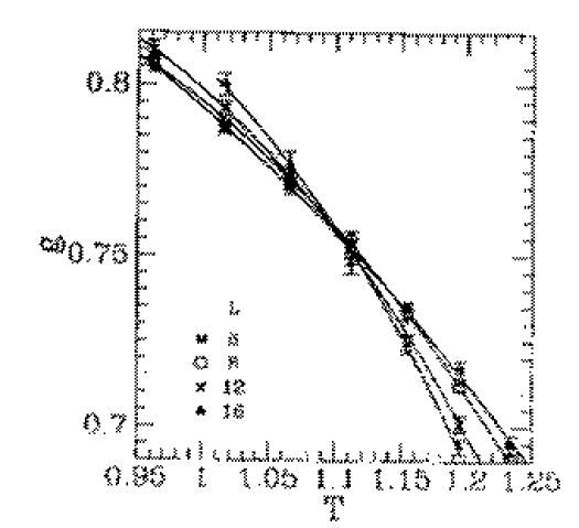
Figure 2: Binder cumulant for the $3D$, $J=\pm 1$ spin glass. From $\!{}^{{\bf?}}$.

One can also use the probability distribution of the overlap, $P(q)$, computed at the critical point, to determine critical exponents. One uses the relation

$$P(q)=L^{\frac{\beta}{\nu}}f\left(qL^{\beta/\nu},L^{\frac{1}{\nu}}(T-T_{c})\right)\ ,$$ (33)

for $T=T_{c}$ to estimate the ratio $\frac{\beta}{\nu}$. We show the result of the best fit in figure (3): one finds $\frac{\beta}{\nu}\simeq 0.3$. The best determination of Kawashima and Young $\!{}^{{\bf?}}$ of the critical value of $T$ and of the critical exponents is $T_{c}^{(\pm 1)}=1.11\pm 0.04$, $\nu=1.7\pm 0.3$ and $\eta=-0.35\pm 0.05$.

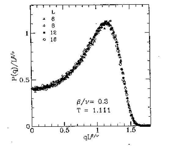
Figure 3: Rescaled $P(q)$ near the critical point for the $3D$ $J=\pm 1$ spin glass. From $\!{}^{{\bf?}}$.

Recent results have been obtained in $\!{}^{{\bf?}}$ by using the parallel tempering Monte Carlo (Appendix 3: Parallel Tempering) to simulate the $3D$ EA first neighbor spin glass model with Gaussian couplings . The use of an improved Monte Carlo technique has allowed to thermalize lattices of size up to $16$ down to $T^{(\min)}\simeq 0.7T_{c}$ (a large gain over what was possible with the standard Monte Carlo approach). In fig. (4) we plot the Binder parameter for $L=4$ and $L=16$ (lower plot), and for $L=8$ and $L=16$ (upper plot). In both cases the crossing is statistically significant in a whole set of $T$ values. It is also interesting to look at the value of the Binder parameter at the critical point, that is an universal quantity: the two cases of $J\pm 1$ and of Gaussian couplings give compatible values, close to $0.75$. This fact constitutes one more evidence for the existence of a phase transition in $3D$.

Figure 4: Binder cumulant for the $3D$ spin glass with Gaussian couplings $\!{}^{{\bf?}}$. In the lower plot $L=4$ and $L=16$, in the upper one $L=8$ and $L=16$.

After establishing the existence of a phase transition in $3D$, we will clarify (mainly after the simulations of $\!{}^{{\bf?}}$) the nature of the cold phase. Again, we are weighting here two possible behaviors: the predictions of Mean Field theory with spontaneous replica symmetry breaking (e.g. a large number of pure states) and the ones from the droplet model (e.g. only two pure states). In order to try and solve this issue we will discuss here about two main sets of observables: i) the behavior of the overlap-overlap correlation function when the overlap is close to zero as a function of space and time; ii) the behavior of the Binder cumulant computed on blocks of different sizes as a function of the block size and of the Monte Carlo time.

Since it is practically impossible to equilibrate very large lattices at very low $T$ values, a shortcut can help: one can for example analyze the dynamic behavior of the system to get information about the equilibrium structure. That is why we are discussing the results of $\!{}^{{\bf?}}$ in this section and not in the section about dynamics: here one uses a dynamic behavior together with an ansatz on the rate of the convergence to equilibrium to get equilibrium information. In the section about off-equilibrium simulations we will describe numerical experiments where one is dealing with quantities that represent intrinsically off-equilibrium phenomena: here, on the contrary, we use off-equilibrium dynamics and a reasonable and verified guess about convergence to equilibrium in order to derive properties of the thermalized system.

So, one $\!{}^{{\bf?}}$ simulates large lattices to avoid the equilibrium situation: starting from random initial conditions one gets a value of the overlap close to zero, that stays close to zero during all the MC run (one needs a huge number of MC sweeps to start and form a macroscopic overlap on a very large lattice $\!{}^{{\bf?}}$).

Let us consider two copies of an infinite system. In practice one takes a system whose size is much larger than $t_{\max}^{{1}/{z(T)}}$, where $z(T)$ is the appropriate dynamic exponent. The overlap $q$ among the two copies at $t=0$ is zero, since one selects two random configurations, and it remains close to zero during all the $t_{\max}$ MC sweeps. In this way the local correlation functions go to a finite limit and they are interpreted to be those of two equilibrium states at $q=0$. It is trivial to verify that in the case of a ferromagnet (or more generally of a system with a unique equilibrium state, neglecting reflections) one finds that

$$G_{x}\rightarrow q_{\rm EA}^{2}\;\;\;{\rm as}\;\;\;x\rightarrow\infty\ ,$$ (34)

where $G_{x}$ has been defined in (15).

At time $t_{0}$ one quenches the system to $T<T_{c}$, and starts measuring the overlap-overlap correlation function $G_{x}(t)$ of eq. (15) (computed now only at time $t$) at distance $x$ and time $t$. At a given time $t$ the system is correlated up to a distance of the order of the dynamic correlation length $\xi(T,t)$, i.e. the correlation functions are statistically different from zero up to this distance. The dynamic correlation length $\xi(T,t)$ grows in time as

$$\xi(T,t)\propto t^{\frac{1}{z(T)}}\ ,$$ (35)

that defines the dynamic critical exponent, $z(T)$ (in the pure Ising model at $T_{c}$ $z=2$, while in the SK model $z(T_{c})=4$). In this way we are trying to verify a power law increase of the dynamic correlation length in all the broken phase, for $T<T_{c}$. $z(T)$ can (and does) depend on the temperature $T$.

The numerical data follow very well the functional form

$$G_{x}(t)=\frac{A(T)}{x^{\alpha}}\exp\left\{-\left(\frac{x}{\xi(T,t)}\right)^{\delta}\right\}\ ,$$ (36)

in a wide rage distance and time regions. Numerical data support this behavior in all the region that has been analyzed, i.e. for $1\leq x\leq 8$, $10^{2}\leq t\leq 10^{6}$ and $0.3~{}T_{c}\leq T\leq T_{c}$. In all these simulations the value of the overlap, $q$, remains very close to zero (since the lattice is large enough as compared to the observation time). One finds that $\!{}^{{\bf?}}$ $z(T)\simeq\frac{6.25}{T}$, an estimate compatible with the results of $\!{}^{{\bf?}}$. For example one estimates $z(T_{c})=6.25\pm 0.30$, in good agreement with the results of $\!{}^{{\bf?}}$($z(T_{c})=6.1\pm 0.3$), the ones of $\!{}^{{\bf?}}$ ($z(T_{c})=5.85\pm 0.30$) and the ones of $\!{}^{{\bf?}}$ ($z(T_{c})=6.0\pm 0.5$). The exponents $\alpha$ and $\delta$ show very little dependence on $T$: for example at $T=0.70$ one finds $\alpha=0.50\pm 0.02$ and $\delta=1.48\pm 0.02$.

Figure 5: $G_{\infty}(x)$ against $x$ in a dilogarithm scale ($T=0.7$). The upper line is the result of a slow cooling while the lower one is obtained after a sudden quench to $T<T_{c}$ (see text).

An effective way to proceed is to take the $t\to\infty$ limit at fixed $x$ on the numerical data, by using the form (36). This procedure gives consistent results, and one obtains in this way data that will be fitted as

$$G_{x}(t=\infty)\equiv\lim_{t\rightarrow\infty}G_{x}(t)=\frac{A(T)}{x^{\alpha}}\ .$$ (37)

We show this correlation function in figure (5) together with the extrapolated correlation function obtained using a cooling procedure. The power law behavior is very clear.

In the mean field framework it is possible to get analytic predictions for these decays. de Dominicis and Kondor $\!{}^{{\bf?}}$ have used RSB theory to compute the $q-q$ correlation function restricted to the $q=0$ sector of the phase space, $G_{x}^{(q=0)}$. One expects a power law behavior, i.e.

$$G_{x}^{(q=0)}\simeq\frac{1}{|x|^{\hat{\alpha}}}\ .$$ (38)

So, there is a good agreement of the expectation generated by the mean field picture and the numerical results: correlation functions in the $q=0$ sector have an equilibrium limit and decay like a power law. These features could not be explained by a droplet model like picture, where there are no $q=0$ equilibrium correlation functions, and the only correlation functions of the theory eventually have to decay to a constant (the square of the EA order parameter, $q_{\rm EA}^{2}$). This evidence is strongly favoring a mean field like picture.

What we have been discussing in the last paragraphs concerns ergodic components of the phase space. We have shown that correlations in the $q=0$ ergodic component of the $3D$ system can be measured, and that one can detect a power law decay, that is what one expects from the mean field theory. We will see now that one can get even stronger evidence that the stable states of the system are organized in a non trivial structure. Thanks to a sum rule we will be able to compare $\!{}^{{\bf?}}$ the full correlation at distance $1$ and the correlation in the $q=0$ sector, and we will show that they are different in the broken phase, for $T<T_{c}$.

In the case of Gaussian couplings, by integrating by parts the expression for the expectation value of the link energy operator it is easy to obtain

$$E_{\rm link}=-\beta(1-G_{x=1})\ ,$$ (39)

that relates the expectation value of the energy (that can be determined with high precision from the numerical data) to the correlation function (integrated over all ergodic components, (27)) at a distance of one lattice spacing.

The value of energy is well determined in the numerical simulation. One can extrapolate to infinite time by using the form $E(t)=E_{\infty}+At^{-\Delta(T)}$. The fit works well: the exponent $\Delta(T)$ is reasonably large. One estimates $\!{}^{{\bf?}}$ that $\Delta(T)=0.44T=\frac{2.75}{z(T)}$. This compares very well a mean field computation $\!{}^{{\bf?},{\bf?}}$ based on the analysis of the interface free energy, where one finds $\Delta(T)\frac{2.5}{z(T)}$: one more quantitative prediction of the mean field theory that describes very well the $3D$ case. One gets a good estimate for $E_{\infty}$. This in turn gives a precise estimate of $G_{x=1}$ One finds that in the high $T$, paramagnetic phase, the $q=0$ correlation functions equals, as expected, the full function, i.e.

$$G_{x=1}^{(q=0)}=G_{x=1}\ ,$$ (40)

where as we have explained we have identified the correlation function measured at short times with the $q=0$ average, and the equality works in the warm phase with a precision better than one percent. On the contrary as soon as we enter in the cold phase the equality (40) is violated: for example at $T=0.7$ one has $G_{x=1}^{(q=0)}=0.612\pm 0.001$ and $G_{x=1}=0.56\pm 0.01$ while at $T=0.35$ $G_{x=1}^{(q=0)}=0.802\pm 0.001$ and $G_{x=1}=0.67\pm 0.01$. This is a strong indication that there are more ergodic components, i.e. that the replica symmetry is broken.

Figure 6: The logarithm of the Binder cumulant for the box overlap versus rescaled ratio of time and distance. Stars are for $R=2$, hexagons are for $R=3$ and asterisk for $R=4$. The straight line is only a guide the eye.

We will describe now a last numerical experiment that is also meant to detect a difference of the DM scenario and the RSB mean field approach. We will see that again a DM approach is falsified from the numerical findings. The experiment is based on studying the quantity $P(q_{R})$, i.e. the probability distribution of the overlap in a box of linear size $R$, $q_{R}$.

In the RSB solution of the Mean Field theory the probability distribution $P(q_{R})$ is Gaussian for $R\rightarrow\infty$, $\frac{R}{L}\ll 1$, while in a DM inspired solution it converges to the sum of two Dirac delta functions (one in $+q_{\rm EA}$ and another in $-q_{\rm EA}$). A practical way to discern among the two possibilities is to look at the Binder cumulant. At time $t$ the cumulant for block of size $R$ is defined as

$$g(R,t)\equiv\frac{1}{2}\left(3-\frac{\overline{\langle q_{R}^{4}\rangle}}{\overline{\langle q_{R}^{2}\rangle}^{2}}\right)\ ,$$ (41)

where $g(R,t)$ is built on data measured after $t$ MC sweeps. ¿From standard dynamic scaling one expects

$$g(R,t)=f(\frac{R}{\xi(t)})\ ,$$ (42)

where $f$ is a scaling function. In figure (6) we show the data for $T=0.7$ and $R=2$, $3$ and $4$. We plot the logarithm of the block Binder cumulant versus $\left(\frac{R}{t^{\frac{1}{z}}}\right)^{\delta}$, by using the exponents $\delta$ and $z$ determined before from the behavior of the overlap-overlap correlation functions (i.e. $\delta=1.5$ and $z=8.3$). The figure makes clear we are not dealing with a $\delta$ function (that would be characterized by $\log(g)=0$): analyzing the system on larger and larger scales we do not find a ferromagnetic behavior, disproving again a droplet like picture.

5.3 Simulations with Three Replicas

One of the potential advantages of using three replicas (i.e. $3$ copies of the system with the same quenched couplings $J$) in a numerical simulation is the possibility of investigating more details of the $P(q)$ (for example by defining new, different Binder cumulant like parameters, and trying to understand if they exhibit a clearer critical behavior: critical exponents are universal, but amplitudes are not). Also, as we will discuss in some detail, working on $3$ replicas helps in getting hints about the metric (or ultrametric) structure of the phase space $\!{}^{{\bf?},{\bf?}}$.

Here we will introduce a Binder cumulant that allows to observe a crossing of curves, plotted as a function of $T$, obtained for different lattice sizes $L$: that strengthens the results about the existence of a phase transition that we have already discussed. In the following (6.5) we will discuss a detailed study of ultrametricity in the $4D$ model done by using a similar approach. Here we are discussing about equilibrium simulations.

Let $\sigma,\tau$ and $\mu$ be three replicas of our $3D$ spin glass: we will simulate them in parallel, using the same quenched disorder (and different random numbers for the dynamic). We will define three different overlaps that we will denote $\{q_{12},q_{23},q_{13}\}$ or $\{q,q^{\prime},q^{\prime\prime}\}$ in the rest of this subsection (where we will mainly follow $\!{}^{{\bf?}}$).

In (20) we have shown one typical relation among expectation values of the probability distribution of the overlap. These relations embody the ultrametric content of the mean field theory $\!{}^{{\bf?},{\bf?}}$. Two specific cases can be written as

$$\overline{\langle q^{2}\rangle^{2}}=\frac{1}{3}\overline{\langle q^{4}\rangle}+\frac{2}{3}\overline{\langle q^{2}\rangle}^{2}\ ,$$ (43)

$$\overline{\langle q^{2}{q^{\prime}}^{2}\rangle}=\frac{1}{2}\overline{\langle q^{4}\rangle}+\frac{1}{2}\overline{\langle q^{2}\rangle}^{2}\ .$$ (44)

Recently Guerra $\!{}^{{\bf?}}$ succeeded to obtain some of these in a rigorous approach to spin glass theory, proving the validity of a set of such relations even for finite dimensional models (constructed by sending to zero a mean-field like perturbation of the Hamiltonian): these results justified the numerical findings of $\!{}^{{\bf?}}$. Both (43) and (44) have been analyzed in detail in $\!{}^{{\bf?}}$: one finds small finite size corrections, and a very satisfactory agreement of the numerical data and the theoretical result in the infinite volume limit. After Guerra $\!{}^{{\bf?}}$ results establishing the numerical validity of (43) and (44) can be considered as a good check of the thermalization (and of the formal correctness of the computer codes!).

As we said by running simulations of $3$ copies of the system one can define more cumulants, that can allow to extract more information about the system. Following $\!{}^{{\bf?}}$ one defines

$$B_{qqq}\equiv\frac{\overline{\langle|q_{12}q_{13}q_{23}|\rangle}}{\overline{\langle q^{2}\rangle}^{3/2}}\ ,\ \ \ \ {B^{\prime}}_{qqq}\equiv\frac{\overline{\langle q_{12}q_{13}q_{23}\rangle}}{\overline{\langle q^{2}\rangle}^{3/2}}\ ,$$ (45)

and

$$B_{q-q}\equiv\frac{\overline{\langle{(|q_{12}|-|q_{13}|)}^{2}\rangle}}{\overline{\langle{q_{23}}^{2}\rangle}}\ ,\ \ \ \ \ {B^{\prime}}_{q-q}\equiv\frac{\overline{\langle{(q_{12}-q_{13}\mbox{ sign}(q_{23}))}^{2}\rangle}}{\overline{\langle{q_{23}}^{2}\rangle}}\ ,$$ (46)

where $q_{23}$ is the largest of the three overlaps (in absolute value). One expects that standard finite size scaling applies:

$$B_{\#}=f_{\#}(L^{\frac{1}{\nu}}(T-T_{c}))\ ,$$ (47)

where we have used the symbol $\#$ to denote one of the cumulants we have just defined. $B_{qqq}$ and $B^{\prime}_{qqq}$ turn out to have the same behavior than the usual Binder cumulant based on two replicas (see figures (2) and (4)). $B_{q-q}$ seems instead to show a clearer signature of the phase transition: in figure (7) we show the $L=4$, $6$ and $8$ data.

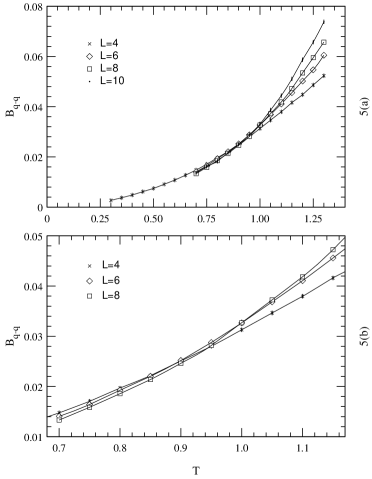
Figure 7: In the upper figure $B_{q-q}$ versus $T$ for $L=4$ to $10$ in a large $T$ range. In the lower one $L=4,6,8$ and $T\in[0.7,1.3]$.

Let us finally quote some preliminary results about the ultrametric structure of the phase space of the $3D$ model $\!{}^{{\bf?}}$. One starts by measuring, after each MC iteration, the $3$ overlap among the $3$ copies of the system, and ordering them in $q_{\max}$, $q_{\mbox{med}}$ and $q_{\min}$. One defines

$$b\equiv\frac{{\left(|q_{\mbox{med}}|-|q_{\min}|\right)}^{2}}{{q_{\max}}^{2}}\ .$$ (48)

One defines the integrated probability $\Pi(b>b_{0})$ by

$$\Pi(b>b_{0})\equiv\int_{0}^{b_{0}}{\rm d}b~{}P(b)\ .$$ (49)

In the small $b_{0}$ region one finds that $\Pi(b_{0})$ decays with a power law, i.e. $\Pi(b_{0})\simeq b_{0}^{-\alpha}$. For intermediate values of $b_{0}$ one sees a fast, exponential decay $\Pi(b_{0})\simeq e^{-\beta b_{0}}$, while in the large $b_{0}$ region $\Pi(b_{0})$ goes to zero faster than an exponential. One can also fix $b_{0}$ (for example by taking $b_{0}=0.05$): $\Pi(b_{0}=0.05)$ decays as power law with the size of the system $L$. In an ultrametric phase space $P(b)$ is a $\delta$ function centered in the origin: these results suggest that ultrametricity holds in $3D$. Also, the theoretical analysis of $\!{}^{{\bf?}}$, based on the results of $\!{}^{{\bf?}}$, shows that if the phase space of a finite dimensional system is ultrametric than necessarily equations like (20,43-46) must hold, i.e. one must find the same ultrametric structure of the mean field solution.

5.4 Out of Equilibrium Dynamics

In the following we will discuss about out of equilibrium dynamics of the $3D$ EA spin glasses. We do not have enough space to give more than basic information: we will be mainly discussing the work by Rieger and coworkers $\!{}^{{\bf?},{\bf?},{\bf?},{\bf?}}$, that the interested reader should consult. The crucial points can be summarized in a few words. In first numerical simulations give results that are completely compatible with the experimental results (concerning, for example, the decay of magnetization after switching off an applied field). Aging phenomena $\!{}^{{\bf?}}$ are clear. In second the most part of results are not compatible with the logarithmic dependence on time implied by the droplet picture. Aging phenomena turn out to be clearly characterized by functions $f(\frac{t}{t_{w}})$ and not, as the droplet model would imply, by functions of $\log(\frac{t}{\tau})/\log(\frac{t_{w}}{\tau})$.

Figure 8: The non-equilibrium exponent ${\lambda(T,t_{w})}$ of the $3D$ EA-model. The straight line is a linear fit of ${\lambda(T)}$ and is a guideline for the eye only. From $\!{}^{{\bf?}}$.

One measures autocorrelation functions at different times, and tries to determine the functional form of the power decay: we will see that numerical results can be well compared to real experimental results. The remnant magnetization, measured at time $t$ after a sudden quench (when a large applied magnetic field is switched off), is defined as

$$M(t)\equiv C(t,0)\ .$$ (50)

Experiments show a clear power law decay, i.e.

$$M(t)\sim t^{-\lambda(T)}\ ,$$ (51)

where $\lambda(T)$ depends on the temperature. In figure (8) we show $\lambda$ versus $T$ (from $\!{}^{{\bf?}}$: the experimental exponents are from $\!{}^{{\bf?}}$). In figure (8) are also the exponents $\lambda(T,t_{w})$, obtained by looking at the decay of $C(t,t_{w})$, for values of the waiting time $t_{w}\ll t$. The data from the real experiment are from the remnant magnetization measurements in an amorphous metallic spin glass. Even if there is a quantitative difference among the numerical and the experimental values the data are very similar (we are discussing about critical exponents, that are always measured with a quite high uncertainty, often more of a systematic than statistical nature).

The autocorrelation function $C(t,t_{w})$ (19) can be analyzed in two different regimes:

• The fully off equilibrium regime (where there is no invariance under time translation), $t\gg t_{w}$ $\!{}^{{\bf?}}$. The asymptotic decay of the remnant magnetization that we have discussed before is a special case ($t_{w}=0$).

• The quasi equilibrium regime that the system reaches for $t\ll t_{w}$.

The behavior of the autocorrelation function in the two cases is well described as

$$C(t,t_{w})\sim\left\{\begin{array}[]{ll}t^{-\lambda(T,t_{w})}&\mbox{ if }t\gg t_{w}\ ,\\ t^{-x(T)}&\mbox{ if }t\ll t_{w}\ .\end{array}\right.$$ (52)

The droplet model would imply in the region $t\gg t_{w}$ a behavior $C(t,t_{w})\sim(\log t)^{-\lambda/\psi}$ that does not describe well the numerical data.

We can write (52) in a compact form by defining a scaling function $f$ such that $C(t,t_{w})=t^{-x}f(t/t_{w})$. The scaling function $f(z)$, tends to a constant when $z\rightarrow 0$ and behaves as $z^{-\lambda+x}$ as $z\rightarrow\infty$: $\lambda$ and $x$ are the exponents defined in equation (52).

The prediction of the droplet model for the correlation function is

$$C(t,t_{w})=(\log t)^{\theta/\psi}g\left(\frac{\log(t/\tau)}{\log(t_{w}/\tau)}\right)\ ,$$ (53)

where $\theta$ and $\psi$ are the droplet model exponents and $\tau$ is a time scale. Also this fit turns out to be inadequate to describe the numerical data. The naive droplet model is definitely falsified from the off-equilibrium dynamic simulations (and from the experimental data). On the contrary mean field theory is characterized by power law decays.

It is also interesting to study the domain growth. One looks at the autocorrelation function among overlaps (see equation (15)). One defines a dynamic correlation length as

$$\xi(t_{w})=2\int_{0}^{\infty}{\rm d}rG_{r}(t_{w})\ .$$ (54)

The dynamic correlation length, $\xi(t_{w})$, turns out to be described very well by an algebraic behavior $\xi(t_{w})\sim t_{w}^{\alpha(T)}$, where the exponent $\alpha$ depends linearly over $T$. In this case also the droplet model behavior $\xi(t_{w})\sim(\log t_{w})^{1/\psi}$ fits the data, with $\psi=0.71\pm 0.02$.

Another interesting result has been obtained in $\!{}^{{\bf?}}$. One computes the ratio between the response ($R(t,t^{\prime})$) and the time derivative of the autocorrelation function $C(t,t^{\prime})$. If the fluctuation-dissipation theorem holds this ratio must be equal to the inverse temperature $\beta$, but in the general case of a complex off-equilibrium dynamics we expect $\!{}^{{\bf?}}$ that

$$\beta\ x_{\rm d}(t,t^{\prime})=\frac{R(t,t^{\prime})}{\displaystyle{\frac{\partial C(t,t^{\prime})}{\partial t^{\prime}}}}\ .$$ (55)

On general grounds one can expect that the a priori arbitrary function $x_{\rm d}(t,t^{\prime})$ would in reality only depend on $C(t,t^{\prime})$ which is the dynamic equivalent of the overlap $q$. In this case $x_{\rm d}(q)$ can be interpreted as the off-equilibrium version of the function $x(q)$ of the static case $\!{}^{{\bf?}}$. Since at equilibrium $q\to q_{\rm EA}$ one recovers the fluctuation-dissipation theorem (since $x(q_{\rm EA})=1$).

6 D=4

The $4D$ case is somehow easier to study numerically than the $3D$ model. The evidence for the existence of a broken phase with a non trivial $P(q)$ and of a mean field like behavior is easy to achieve. Because of that the $4D$ model will be discussed here from two points of view. In first it will be seen as the model where firm evidence for the mean field pattern to apply in finite number of dimensions has been established. In second it will be discussed as the model where more difficult questions, like the existence of an ultrametric organization of the phase space, start to be analyzed in detail.

6.1 Close to the Phase Transition

First Bhatt and Young $\!{}^{{\bf?},{\bf?},{\bf?}}$ noticed that in the $4D$ EA model one can locate $T_{c}$ with a relatively small amount of computational work.

In $4D$ the curves representing the overlap Binder cumulant as a function of $T$, for different size values $L$, cross very clearly giving a precise estimate of $T_{c}$ (as a function of increasing lattice size the cumulant tends to zero from above in the warm phase, and to a non-trivial, non-zero value from below in the broken phase: the $T$ point where different $L$ curves cross is a good finite size estimate of the infinite volume $T_{c}$). The very clear crossing (a behavior similar to the one seen in the SK model or, for the magnetization cumulant, in the $3D$ Ising model) allows a precise estimate of $T_{c}$ ($T_{c}=2.02\pm 0.03$ for $J=\pm 1$, $T_{c}=1.75\pm 0.05$ for Gaussian couplings: see $\!{}^{{\bf?},{\bf?},{\bf?}}$ and the more recent simulations of $\!{}^{{\bf?}}$, done using the dedicated parallel computer RTN $\!{}^{{\bf?}}$).

The value of the critical exponent $\nu$ turns out to be quite small (about $0.8$). This value is nearly a factor $2$ smaller that the three dimensional value and this implies that on a finite lattice we can go much closer to the critical point by keeping finite size effects small.

6.2 Below the Transition

The most interesting results have been obtained by simulations done below the phase transition point. The measurements of the overlap probability distribution $P(q)$ can be done at $T<T_{c}$ much easily than in the three dimensional case. Finite size effects turn out to be large (this is already true in the SK model, and stays true three dimensions: it looks like an intrinsic problem of systems with quenched disorder). The variation of $P(q)$ as function of the lattice size (for $L$ going from 3 to 7) is of the same order of magnitude than the one one finds in three dimensions) $\!{}^{{\bf?},{\bf?}}$.

Thermalization is faster here than in $3D$ and good quality results in a large region of the broken phase have been obtained by using simple minded Monte Carlo techniques. The probability distribution of the energy overlap converges in the infinite volume limit to a non trivial function.

The difference in the crossing properties of the Binder parameter in four and in three dimensions has clear origin. If replica symmetry is spontaneously broken, in the infinite volume limit the Binder parameter converges to a non trivial function of $T$, $g(T)$. In the mean field theory $\!{}^{{\bf?}}$the function $g(T)$ for $T<T_{c}$ is approximately given by $1-.4{\theta(1-\theta)}$ (we have defined by $\theta$ the reduced temperature, $\theta\equiv\frac{T}{T_{c}}$). In other words $g_{-}\equiv\lim_{T\to T_{c}^{-}}g(T)$ is $1$, which is quite different from the value of the Binder parameter at the crossing point (which is close to .3, as can be seen by numerical simulations of the SK model $\!{}^{{\bf?}}$).

When we go in less than $6$ dimensions the quantity $g_{-}$ starts to be less than one and decreases with the dimensionality of the space. When, by decreasing $D$, the value of $g_{c}$, i.e. the value of the Binder cumulant at the crossing point becomes close to $g_{-}$, the effect of crossing becomes very difficult to detect $\!{}^{{\bf?}}$. One also expects that $g_{c}$ becomes a non trivial function of $D$ for dimensions lower than 6.

This behavior is related to the lack of scaling in the mean field theory. Indeed the function $P(q)$ can be written as

$$P(q)=\tilde{P}(q)+(1-x_{M})\delta(q-q_{\rm EA})$$ (56)

where the term $\tilde{P}(q)$ does not contain a delta function at $q_{\rm EA}$. The quantity $x_{M}$ gives the probability of finding two different systems with an overlap $q<q_{\rm EA}$. In mean field theory $x_{M}$ is proportional to $T_{c}-T$: since a pure number is proportional to the distance from the critical temperature scaling is badly violated. On the other end it was shown $\!{}^{{\bf?}}$ that in less than $6$ dimensions scaling is restored and the function $P(q)$ scales as

$$q_{\rm EA}P(q)=f(\frac{q}{q_{\rm EA}})\ ,$$ (57)

where $q$ vanishes as a $|T-T_{c}|^{\beta}$. At least a partial verification $\!{}^{{\bf?}}$ of equation (57) has been done by verifying that near $T_{c}$ the quantity $q_{\rm EA}P(0)$ does not depend on $T$.

6.3 Non-Zero Magnetic Field

An important prediction of the mean field solution concerns the existence of a transition even for non zero magnetic field. When the magnetic field is small enough it exists a $h$ dependent temperature $T_{\rm AT}(h)$ (the de Almeida-Thouless line) where the overlap susceptibility diverges. Below the field dependent critical temperature the function $P(q)$ is non trivial.

It is difficult to study numerically the transition in field in good detail $\!{}^{{\bf?},{\bf?},{\bf?},{\bf?}}$. The function $P(q)$ is symmetric around the origin at $h=0$, and it is concentrated at positive $q$ values for non zero $h$. If $h$ is too small and the volume is not too large, one finds a tail of configurations with negative $q$. This tail disappears when increasing the volume, but complicates the analysis $\!{}^{{\bf?},{\bf?},{\bf?}}$. This region is relevant for the cross-over behavior from $h=0$ to $h\neq 0$. If $h$ is not so small (for example for an $h$ such to induce a magnetization of $0.15$), the critical temperature is decreased by a large factor as compared to the $h=0$ case (of circa $40\%$ in the specific case of $m=0.15$) and in this low temperature region measurements are much more difficult .

The present data $\!{}^{{\bf?},{\bf?}}$ support the existence of a transition: at low temperatures the overlap susceptibility diverges roughly proportionally to the volume and the function $P(q)$ strongly fluctuates from system to system. Studies of the system in presence of an external field (conjugated to the overlap) which couples two replicas suggest the presence of discontinuities at $\epsilon=0$, but a relative large extrapolation is needed for reaching these conclusions.

Unfortunately for $h\neq 0$ the values of the various Binder cumulants (related to skewness and kurtosis) as a function of the temperature have a rather complex behavior, and it is not clear how to use them to locate the phase transition point. Also the theoretical situation is very confused: the renormalization group predictions for the critical exponent cannot be computed because no fixed point has been found $\!{}^{{\bf?}}$. The result is puzzling and no convincing interpretations have been yet presented.

We believe that a much more careful study of the properties at non zero magnetic field above and below the De Almeida-Thouless line is very important and the present situation can be strongly improved in the next future.

6.4 Out of Equilibrium Dynamics

We will discuss here, again (see (5.4)), an out of equilibrium approach. In some situations that can be very helpful (we will see that in the $4D$ case we can even measure $q_{\rm EA}$ by an off-equilibrium technique). Here one measures the relevant quantities as a function of time. Often they can be fitted extremely accurately, in a large time window, by power laws, i.e. by a form $A+Bt^{-C}$: in this way, especially if the exponent $C$ is not too small, one can perform the $t\to\infty$ limit quite precisely. One further advantage of the method is that one can work with very large lattices. Taking a lattice size much larger that the dynamic correlation length allows to make finite size corrections very small.

In the following we will mainly focus on the relation between off and on equilibrium regimes, by describing mainly the work of $\!{}^{{\bf?}}$. We will see that it will be possible to establish strong links between the two regimes.

Asymptotically an equilibrium situation is reached by making $t_{w}$ large in the correlation functions of (19) (so that the system is at equilibrium on very large time scales), and then considering large, but small compared to $t_{w}$, measuring times $t$. In this case we can expect to find power like corrections to $q_{\rm EA}$. We can write

$$q(t)\equiv\lim_{t_{w}\rightarrow\infty}C(t,t_{w})=\left(q_{\rm EA}+at^{-x}\right)\;\;\;\mbox{for}\;\;t\gg 1\ .$$ (58)

Here we are saying that if we wait a large time the system will be equilibrated on time scales smaller than the waiting time. So if we measure correlations up to these scales we will find that the autocorrelation function tends to a plateau that is exactly the Edwards-Anderson order parameter: for $t\simeq t_{w}$ there will be a crossover, and the correlation function will decay to zero. The most part of numerical simulations, done in a region of short waiting times, were dealing with this second regime $\!{}^{{\bf?},{\bf?},{\bf?}}$, observing a power decay to $q=0$. Using a large waiting time has recently allowed $\!{}^{{\bf?}}$ to clearly detect the effect implied by (58).

One uses a large $\frac{t_{w}}{t}\geq 32$ ratio. In these conditions the numerical data are well fitted by the form

$$C(t,t_{w})=(q_{\rm EA}+at^{-x})\ \overline{C}(\frac{t}{t_{w}})\ ,$$ (59)

where for $z\to 0$ one has $\overline{C}(z)\simeq 1-c_{1}z^{\zeta}$. One first determines the rescaling function $\overline{C}(\frac{t}{t_{w}})$ by fitting the numerical data for the autocorrelation function at a fixed value of $t$ (as a function of $t_{w}$). Then one divides away from the numerical data the value of $\overline{C}$: the fact that all the rescaled points, at different $t$ and $t_{w}$, fall on a single, universal curve, is a test of the fact that (59) was a correct Ansatz.

After these steps one can try to fit the scaling curve to a power behavior. The numerical date together with the fit are shown in figure (9).

Figure 9: $C(t,t_{w})/\overline{C}(t,t_{w})$ versus $t$ at $T=0.9$. The dashed line is the pure best power fit while the solid line is the best power fit including a constant: $(0.60\pm 0.04)+(0.32\pm 0.04)t^{-0.08\pm 0.01}$. From ref. $\!{}^{{\bf?}}$.

It is clear from this figure that for large $t$ (but still in the regime $t_{w}/t\geq 32$), the data do not follow a pure power fit ($t^{-x}$) and there is a correction that can be taken in account by fitting to the form $q_{\rm EA}+at^{-x}$. In figure 9 we also plot this second fit.

The best estimates for $q_{\rm EA}$ as a function of $T$ are shown in (10). The dashed line is the function

$$q_{\rm EA}(T)\simeq\left(\frac{T_{c}-T}{T_{c}}\right)^{\beta}.$$ (60)

drawn using the values obtained by equilibrium simulations of the model $\!{}^{{\bf?}}$: $T_{c}=1.8$ and $\beta=0.74$. The line is only a guide to the eye, but it coincides very well with the numerical data, even far from $T_{c}$ (where we do not expect a priori that a simple power decay holds).

Figure 10: $4D$ Edwards-Anderson order parameter, computed from non-equilibrium dynamics, versus $T$. From ref. $\!{}^{{\bf?}}$.

6.5 Ultrametricity

Verifying the ultrametric structure of spin glass models by numerical simulations is a difficult task. Even for the SK model, where we know analytically what to expect, fully satisfactory numerical checks have not been yet obtained. Still, the question is very important: is the phase structure of finite $D$ models reminiscent of the ultrametric organization of the mean field solution? Cacciuto, Marinari and Parisi $\!{}^{{\bf?}}$ have discussed this issue in the $4D$ case, and found a positive evidence, that we will discuss in the following. The interested reader can read the interesting introductions and discussions of $\!{}^{{\bf?},{\bf?}}$: mean field techniques allow advanced computations about the ultrametric structure of the phase space $\!{}^{{\bf?},{\bf?}}$.

A good introduction to ultrametricity for physicists is in $\!{}^{{\bf?}}$. Here we just remind the reader that the usual triangular inequality

$$d_{1,3}\leq d_{1,2}+d_{2,3}\ ,$$ (61)

is substituted in spaces endowed with an ultrametric distance by the stronger inequality

$$d_{1,3}\leq\max\left(d_{1,2},d_{2,3}\right)\ .$$ (62)

In an ultrametric space all triangles have at least two equal sides, that are larger or equal than the third side. An hierarchical tree is a very good way of representing an ultrametric set of states. In the solution of the mean field spin glass theory one finds an exact ultrametric structure: states are organized on an hierarchical tree, and if we pick up three equilibrium configurations of the system and compute their distance we find an ultrametric triangle.

Reference $\!{}^{{\bf?}}$ is based on a constrained Monte Carlo procedure. One updates three replicas of the system (in the same set of couplings), and constrains the distance of replica one and replica two to a given value $q_{1,2}$, and the distance of replica two and replica three to $q_{2,3}$ (that can be equal to $q_{1,2}$). We have three replicas, two distances are fixed and we measure the third one, that we call $q$. For example if one fixes both values to some fraction of $q_{\rm EA}$ (in the case of $\!{}^{{\bf?}}$ to $\frac{2}{5}q_{\rm EA}$) an ultrametric structure would imply that $q\geq\frac{2}{5}q_{\rm EA}$, while the usual triangular inequality would only imply that $q\geq-\frac{7}{5}q_{\rm EA}$. Obviously the choice of the constraint is crucial to obtain a sharp difference from the usual situation of an Euclidean metric.

It has been possible to thermalize lattices of up to $8^{4}$. The computation turns out to be, as we will see, very successful. The most serious problem turns out to be in the usual finite size effects: finite size effects are serious in spin glass models, and in this computation they appear clearly. In order to be more quantitative we define the integral

$$I^{L}\equiv\int_{-1}^{q_{\rm min}}{\rm d}q~{}\left(q(L)-q_{\rm min}\right)^{2}\ P(q)\ +\int_{q_{\rm max}}^{+1}{\rm d}q~{}\left(q(L)-q_{\rm max}\right)^{2}\ P(q)\ ,$$ (63)

where $q_{\rm min}$ is the minimum $q$ allowed (for us, for example, $q_{\rm min}=q_{1,2}$), and $q_{\rm max}=q_{\rm EA}$. $I^{L}$ goes to zero if the system is ultrametric. We plot $I^{L}$ in fig. (11) for the two choices of the constraint that have been discussed in $\!{}^{{\bf?}}$.

Figure 11: The integral $I^{L}$ as a function of $L$, in double log scale. The lower points are for the case where we have fixed $q_{1,2}=q_{2,3}$, the upper points where $q_{1,2}\neq q_{2,3}$ (see the text).

For example in the case of two equal distances a very good best fit shown in the figure gives

$$I^{L}\simeq(-0.0001\pm 0.0005)+(0.76\pm 0.03)L^{-2.21\pm 0.04}\ .$$ (64)

It is remarkable that the mean field computations of $\!{}^{{\bf?},{\bf?}}$ give an exponent of $\frac{8}{3}\simeq 2.67$, for the deviations from a pure ultrametric behavior in a finite system. Not only one finds a system that for large $L$ is converging to an ultrametric behavior, but the rate of the convergence is very similar to the one one can compute in the mean field model. This is one of the quantitative agreements that make the relation of the mean field solution and the finite dimensional models clear and impressive.

7 D=2

We do not have enough space to enter in many details about the $2D$ case $\!{}^{{\bf?},{\bf?},{\bf?},{\bf?},{\bf?},{\bf?},{\bf?},{\bf?}}$. We will briefly discuss the statics of the problem, the out off-equilibrium dynamics and try to stress some important points, like the nature of the $T=0$ divergence.

7.1 Statics

As we have discussed the original Bhatt and Young work $\!{}^{{\bf?}}$ seems already to shed a clear light on the $2D$ cases (we will discuss in a few lines recent doubts $\!{}^{{\bf?}}$). For $J=\pm 1$ couplings one was finding a clear signature for a $T=0$ transition, with power law divergences with $\nu=2.6\pm 0.4$, $\eta=0.20\pm 0.05$ and $\gamma=4.6\pm 0.5$.

Recent transfer matrix calculations $\!{}^{{\bf?}}$, mainly looking at the complex zero structure of the partition function, seem however to be opening doubts, supporting a correlation length that would be diverging exponentially (see also our discussions of section (5)). So one would have that (for $J=\pm 1$ in $2D$) $\xi\simeq\exp(\frac{2}{T})$. The question does not seem to be solved at the moment.

The model with Gaussian couplings $J$ has been discussed in detail in $\!{}^{{\bf?}}$, under the two aspects of the $T=0$ structure and of the finite $T$ equilibrium. $T=0$ has been analyzed by determining ground states thanks to a branch and cut algorithm. Under this approach the authors find $y=-.281\pm 0.002$ (and since one expect $y=\frac{1}{\nu}$ that gives $\nu=3.56\pm.02$). A Monte Carlo simulation is used to determine the finite $T$ behavior. Assuming a $T=0$ power law divergence and using continuous couplings (with no accidental degeneracy) one has that $\eta=\beta=0$ and $\frac{\gamma}{\nu}=2$, leaving only one independent exponent, say $\nu$, to be determined. In fig. (12) we show the susceptibility from ref. $\!{}^{{\bf?}}$, and the good finite size scaling behavior obtained by using $\nu=3.45$.

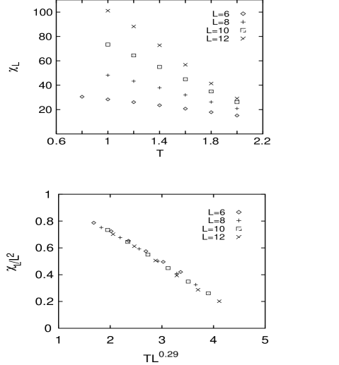
Figure 12: $2D$ Gaussian $J$ spin glass: equilibrium values of the susceptibility depending on temperature and system size. In the upper figure the bare data, in the lower part the rescaled data.

By also using a detailed analysis of the Binder parameter $g$ one gets $\nu=3.6\pm 0.02$, in very good agreement with the $T=0$ result for $y$. Ref. $\!{}^{{\bf?}}$ also give a quite precise estimate of the magnetization exponent $m_{\infty}(h)\simeq h^{\frac{1}{\delta}}$, $\delta=1.48\pm 0.01$ (there is a problem since one would expect $\delta=1-y$, that is not well verified by the data). Also they study the chaotic behavior one expects in spin glasses. Also a very recent paper $\!{}^{{\bf?}}$ is based on $T=0$ exact ground states, and allows a determination of the stiffness exponent, that turns out to be small and negative, $-0.056\pm 0.006$.

At last we note that Lemke and Campell $\!{}^{{\bf?}}$ have studied the $2D$ model with next-nearest neighbor interactions and found signs of the possible existence of a spin glass phase.

7.2 Out of Equilibrium Dynamics

We will give here a few details about the off equilibrium dynamics in the $2D$ model, by mainly following $\!{}^{{\bf?}}$ and $\!{}^{{\bf?}}$. The main points are maybe that interrupted aging can be observed in detail (since there is no phase transition the system eventually converges to a time translational invariant regime), and that again the predictions of the droplet model do not fit the numerical data. As usual, the numerical studies are mainly based on the measurement of the correlation function defined in equation (19).

The first result, see figure (13) ), is that for waiting times $t_{w}$ larger than a given value $\tau_{\rm eq}$ the curves of the autocorrelation function, $C(t,t_{w})$, as a function of $t$ for different $t_{w}$, collapse. This implies that the system equilibrates. One can identify $\tau_{\rm eq}$ as the time necessary to reach the equilibrium situation (the regime where the fluctuation-dissipation theorem holds). This is what is called interrupted aging. The equilibration time grows when the temperature decreases. For lower temperatures the equilibration time becomes larger that the simulated time and the situation is not qualitatively different from the one three or four dimensions.

Figure 13: Autocorrelation function $C(t,t_{w})$ as a function of time $t$ for $t_{w}=5^{n}$ ($n=1,\ldots,8$) at $T=1.0$ and $0.8$, ($n=2,\ldots,8$) at $0.6$ and $0.2$. The system size is $L=100$ and the disorder average was performed over 256 samples. The error bars are smaller than the symbols. From ref. $\!{}^{{\bf?}}$.

The correlation function, $C(t,t_{w})$, follows empirically the scaling law

$$C(t,t_{w})=f(\frac{t}{\tau(t_{w})})\ ,$$ (65)

where $f(x)$ is a scaling function and the time scale, $\tau(t_{w})$, is proportional to $t_{w}$ as $t_{w}\ll\tau_{\rm eq}$, and reaches a plateau when $t_{w}>\tau_{\rm eq}$. In the latter regime the variable of the scaling function will be $\frac{t}{t_{w}}$. The droplet model suggests a dependence over $\frac{\log(t)}{\log(t_{w})}$ that is clearly unable to describe the data.

Also measurements of the correlation length $\xi(t_{w})$ give precise results. The fit to a pure algebraic behavior, $\xi\propto t^{\alpha(T)}$, with $\alpha\simeq 0.2T$ works well. The droplet approach predicts $\xi(t_{w})\propto(\log t_{w})^{1/\psi}$, that here also gives a reasonable fit, with $\psi=0.65\pm 0.01$ independent of $T$.

Appendix 1: On the Definition of Pure States.

We will give here a few more details about the problem of defining pure states. We will use this notion in a physical way, which may be different from the approach used by the mathematical physics community.

The basic idea is rather simple. Let us consider for simplicity a spin system with nearest neighbor interaction on the lattice. Everything works fine for an actually infinite system. We define a state $\rho(C)$ as a probability distribution over the configurations $C$ of the infinite system . A state is said to be a local equilibrium state (or a DLR state $\!{}^{{\bf?}}$) if the restriction to a finite volume of the probability distribution that characterizes it is given by the Boltzmann formula.

A theorem says $\!{}^{{\bf?}}$ that any DLR state can be decomposed as the sum, with non negative coefficients, of pure DLR states:

$$\langle\cdot\rangle=\sum_{\alpha}W_{\alpha}\langle\cdot\rangle_{\alpha}\ .$$ (66)

Pure states are the ones for which the only possible decomposition has one $W_{\gamma}=1$ and all the other weights equal to zero. In other words the DRL states are a convex set and the pure states are the extremal states of this set. The pure states can also be characterized by the clustering property: in pure states the connected correlations functions go to zero at large distances, or equivalently in pure states intensive quantities do not fluctuate $\!{}^{{\bf?},{\bf?}}$ .

The proofs which are needed are very simple if one uses the appropriate mathematical setting $\!{}^{{\bf?}}$. Hard problems start when we have to show that this nice construction is not empty, i.e. when we have to prove that local equilibrium states do exist for the infinite system. The simplest way we have to accomplish this task is to take a finite volume system and to show that the infinite volume limit of the Boltzmann Gibbs probability does exist and it is a local equilibrium state. In this construction there is the freedom to chose the boundary conditions of the system, that could lead to different local equilibrium states. If the boundary conditions are chosen in an appropriate way (e.g. all spins up in a ferromagnet) a pure state is obtained.

This decomposition into pure states is well known. It was developed thirty years ago for the case of translational invariant Hamiltonians $\!{}^{{\bf?}}$. In the case of spin glasses (and more generally of other system with quenched non translationally invariant disorder) things are much more difficult. The very concept of a probability distribution over configurations of the actually infinite system needs extreme mathematical care. Just consider the example of a ferromagnet at low temperature in presence of a random quenched magnetic field. We know that for a finite, large system, there is a magnetization which is equal to $\pm 1$, the sign being the one of $h_{T}\equiv\sum_{i}h_{i}$, provided that $h_{T}^{2}$ is a quantity of order of the volume (as usually happens). Everything is clear! However if we want to consider an actually infinite system which is the sign of $h_{T}$? We could consider the function $s(L)\equiv\mbox{ sign}\sum_{i=-L,L}h_{i}$, but this leads nowhere because if the $h_{i}$ are random variables with zero average, $s(L)$ does not have a limit when $L$ goes to infinity.

The real problem with spin glasses and with other disordered systems is that it is extremely difficult to control the Boltzmann Gibbs probability in the infinite volume limit. The previous example of a ferromagnet in a random field strongly suggests that such limit may not exist, at least not in a naive way. Similar conclusions are valid for spin glasses in the mean field approach $\!{}^{{\bf?}}$, and they have been conjectured to be valid also for short range glasses. Sometimes one refer to this phenomenon as chaotic dependence of the properties of the system on the size $\!{}^{{\bf?}}$. To deal with this problem different techniques have been suggested (for a recent discussion see reference $\!{}^{{\bf?}}$). Using different definitions leads to different results, that potentially describe very different physical pictures $\!{}^{{\bf?},{\bf?}}$.

A decomposition into pure states of the Boltzmann Gibbs probability distribution for an infinite system is only possible if the Boltzmann Gibbs probability distribution exists in the infinite volume limit and this does not seem to be the case of many disordered systems. An alternative approach consists in making an approximate decomposition into pure states for a finite system; this decomposition must coincide with the usual definitions in the case where the infinite volume limit can be done without difficulties (i.e. where there is no chaotic dependence on the side).

Let us see how one could define approximate pure states in a large but finite system. In this way we are giving a different, but maybe more physical, definition of a state.

Let us consider a system in a box of size $L$. We partition the configuration states in regions, labeled by $\alpha$, and we define the averages restricted to these regions $\!{}^{{\bf?},{\bf?}}$. We have to impose that the restricted averages on these two regions are such that connected correlation functions are small at large distance $x$, i.e. they go to zero faster than a given function $A(L)$ such that $\lim_{L\to\infty}A(L)=0$. In this way we recover eq. (66) for a finite system. In the case of a ferromagnet the two regions are defined by considering the sign of the total magnetization. There are ambiguities with those configurations which have exactly zero total magnetization, but the probability that such a configuration occur is exponentially small at low temperature.

Physical intuition tells us that this decomposition can be done (at least for familiar systems), otherwise it would make no sense to speak about the spontaneous magnetization of a ferromagnetic sample or to declare that a finite amount of water (at the melting point) is in the solid or liquid state (also all numerical simulations gather data that are based on these kinds of notions, since systems we can store in a computer are always finite). We strongly believe that these statements do make sense, although their translation in a rigorous mathematical setting has never been done (as far as we known) also because it is much simpler (and in many cases sufficiently enough) to work directly in the cozy infinite volume setting.

We assume that such decomposition can be done also in spin glasses (the contrary would be highly surprising for any system with a short range Hamiltonian). Therefore the finite volume Boltzmann Gibbs measure can be decomposed in sum of the finite volume pure states according to the previous definitions. The states of the system are labeled by $\alpha$ and they satisfy eq. (66). The function $P(q)$ for a particular sample is given by

$$\sum_{\alpha,\beta}W_{\alpha}W_{\beta}\delta(q_{\alpha,\beta}-q)\ ,$$ (67)

where $q_{\alpha,\beta}$ is the overlap among two generic configurations in the state $\alpha$.

This definition of states is used only at a metaphorical level. The predictions of the mean field theory concerns correlation functions computed in the appropriate ensemble $\!{}^{{\bf?}}$ and computer simulations measure directly these correlation functions. The decomposition into states (which is never done explicitly during computer simulations) is an interpretative tool which describes the complex phenomenology displayed by the correlation functions in a simple and intuitive way. We could alternatively define the function $P(q)$ as

$$\int dqP(q)q^{s}={\sum_{i,k=1,N}<\sigma_{i}\sigma_{k}>^{2s}\over N^{2}}\ ,$$ (68)

but this definition would have much less intuitive appeal the previous one.

The two approaches, the replica analysis of the finite volume correlations functions (and the results which can be stated in a simple and intuitive way by using the idea of decomposition into states of the Boltzmann Gibbs measure) and the construction of pure states for the actually infinite system, give complementary information which can be hardly compared one with the other. In the replica method one obtains information only on those states whose weight $w$ does not vanish in the infinite volume limit . All local equilibrium states have the same free energy density; however the differences in the total free energy may grow as $L^{(D-1}$. From an infinite volume point of view all these states are equivalent, from a finite volume point of view only the state with lower free energy and the states whose total free energy differ from the ground states by a finite amount are relevant.

For example in the ferromagnetic case (in more than two dimensions at sufficient low temperature) there are equilibrium states which have in half of the infinite volume positive magnetization and in the other half negative magnetization. These states are invisible in the replica method because their weight (when restricted to a finite volume system) goes to zero as $\exp(-A\L^{D-1})$ (special techniques, i.e. coupling replicas may be used to recover, at least partially, this information). In the replica method the states are weighted with the corresponding Boltzmann Gibbs weight and this weight can be hardly reconstructed from an analysis done directly at infinite volume.

Appendix 2: Simulated Tempering

In this section we will describe the so called tempering methods $\!{}^{{\bf?}}$ (see also the lecture notes in $\!{}^{{\bf?}}$). In these methods the temperature becomes a dynamic variable. In particular we will describe the simulated tempering method $\!{}^{{\bf?}}$ and a crucial variation, the powerful parallel tempering scheme $\!{}^{{\bf?},{\bf?}}$. The multicanonical methods $\!{}^{{\bf?},{\bf?}}$ have very similar roots, and can be also employed very effectively, but we will not describe them here. These methods has been used to simulate very effectively a wide range of physical problem (see $\!{}^{{\bf?}}$ for a list).

The basic idea of both methods is to move in the temperature space (always staying at thermodynamical equilibrium with respect to a suitable probability distribution) to avoid being trapped fro high energy barriers: the system change its temperature, goes up to the paramagnetic phase and eventually goes back to the lower temperatures. With high probability in different visits the system will visit new local minima (if the phase space has a reasonable shape).

Let us introduce the tempering scheme. We have the original phase space, that we will denote by {X}, a Hamiltonian ${\cal H}(X)$ and a new variable $m$ which takes $M$ values ($\{m\}=\{1,...,M\}$). We extend the original phase space to a new space $\{X\}\times\{m\}$. The probability for a element, $(X,m)$, of this extended phase space to occur is given by

$$P(X,m)\equiv\frac{1}{{\cal Z}_{\rm EXT}}\exp\left[-{\cal H}_{\rm EXT}(X,m)\right]\ ,$$ (69)

where

$${\cal H}_{\rm EXT}(X,m)\equiv\beta_{m}{\cal H}(X)-g_{m}\ ,$$ (70)

and

$${\cal Z}_{\rm EXT}\equiv\sum_{m=1}^{M}\sum_{\{X\}}\exp\left[-{\cal H}_{\rm EXT}(X,m)\right]=\sum_{m=1}^{M}e^{g_{m}}{\cal Z}(\beta_{m})\ .$$ (71)

The extended partition function is the weighted sum of the $M$ partition functions (${\cal Z}(\beta_{m})$) at given $\beta_{m}$, and

$${\cal Z}(\beta_{m})\equiv\sum_{\{X\}}\exp\left[-\beta_{m}{\cal H}(X)\right]\ .$$ (72)

The $\beta_{m}$ are dynamic variables which will be allowed to span a set of given values (e.g. the inverse temperatures that we want to simulate) and the $g_{m}$ must be fixed before the run begins.

If we fix $m$, it is obvious that the probability distribution for $X$ is given by the usual Boltzmann weight with $\beta=\beta_{m}$. Moreover, the probability to find a given value of $m$ is

$$P(m)\equiv\sum_{\{X\}}P(X,m)=\frac{{\cal Z}(\beta_{m})e^{g_{m}}}{{\cal Z}_{\rm EXT}}=\frac{1}{{\cal Z}_{\rm EXT}}\exp(-\beta_{m}f(\beta_{m})+g_{m})\ ,$$ (73)

where $f(\beta_{m})$ is the free energy at fixed $m$ (i.e. $\beta_{m}f(\beta_{m})=-\log{\cal Z}(\beta_{m})$).

If we choose $g_{m}=\beta_{m}f(\beta_{m})$ all the different $m$’s have the same probability, equal to $1/{\cal Z}_{\rm EXT}$. In this case ${\cal Z}_{\rm EXT}=M$.

Now, we will compute the probability of jumping between two consecutive inverse temperatures $\beta_{m}$ and $\beta_{m+1}$ (we are assuming that the $\beta$’s are ordered: $\beta_{m}<\beta_{m+1}<\beta_{m+2}<\ldots$). The variation of the extended Hamiltonian for a given configuration $X$ is

$$\Delta{\cal H}_{\rm EXT}=E_{\rm inst}\delta-(g_{m+1}-g_{m})\ ,$$ (74)

where $\delta\equiv\beta_{m+1}-\beta_{m}$ and $E_{\rm inst}$ is the instantaneous energy, $E_{\rm inst}\equiv{\cal H}(X)$. Expanding $g_{m+1}=\beta_{m+1}f(\beta_{m+1})$ near $\beta_{m}$ we obtain

$$g_{m+1}\equiv g(\beta_{m+1}) = g(\beta_{m})+\left.\frac{dg(\beta)}{d\beta}\right|_{\beta=\beta_{m}}\delta$$ (75)

$$+ \frac{1}{2}\left.\frac{d^{2}g(\beta)}{d\beta^{2}}\right|_{\beta=\beta_{m}}\delta^{2}+O(\delta^{3})$$

$$= E(\beta_{m})\delta+\frac{1}{2}C(\beta_{m})\delta^{2}+O(\delta^{3})\ ,$$

where $E(\beta_{m})$ is the mean energy at $\beta_{m}$, $dg(\beta)/d\beta=E(\beta)$ and $dE/d\beta=C(\beta)\equiv\langle{\cal H}^{2}\rangle-\langle{\cal H}\rangle^{2}$.

By assuming that $E_{\rm inst}$ is close to $E(\beta_{m})$, the variation $\Delta{\cal H}_{\rm EXT}$ will be not large if we keep $C(\beta_{m})\delta^{2}=O(1)$. In this case we will have a reasonable acceptance ratio for the $\beta$ swaps. This condition of $\delta$ is equivalent to impose that the energy histograms at $\beta_{m}$ and $\beta_{m+1}$ overlap.

At the critical point the specific heat ($C(\beta)$) diverges as

$$C(L,\beta_{c})\propto L^{\alpha/\nu+d}\ ,$$ (76)

such that the condition on $\delta$ reads

$$\delta\propto L^{-(d+\alpha/\nu)/2}\ ,$$ (77)

while in the non critical region $C(L,\beta)$ diverges with the volume, $L^{d}$, and

$$\delta\propto L^{-\frac{d}{2}}\ .$$ (78)

The procedure used in the tempering method is composed by two steps (we start the update from $(X,\beta_{k})$):

1. We update the spin configuration $X$ to $X^{\prime}$ using, for instance, the Metropolis or Heat Bath method at fixed $\beta_{k}$. We can repeat this step a certain number of times before going to the next phase.

2. We try to update the inverse temperature $\beta_{k}$ to $\beta_{k\pm 1}$ using a Metropolis like test: if $\Delta{\cal H}_{\rm EXT}<0$ we accept the change, otherwise we accept the change with probability $\exp(-\Delta{\cal H}_{\rm EXT})$.

This procedure satisfies detailed balance. From the previous discussion it should be clear that the most difficult part of the method is to fit the $g_{m}$ to the values of the free energies (on the contrary selecting the $\beta$ set is not a very demanding task). This can be done by using an iterative procedure inside the simulating program: we change at run time the $g_{m}$ values until we obtain an uniform probability for the different $\beta$’s.

A typical run done using this method consists in:

1. Run a simple Metropolis algorithm in order to get a first calculation of the free energies.

2. Run the simulated tempering and change, at run time, the previous values of the free energies in order to obtain a constant probability on $\beta$’s.

3. Run the equilibrium simulations, with fixed $g_{m}$, and measure the interesting observables.

Appendix 3: Parallel Tempering

A great improvement to the previous method is the parallel tempering method (PT) $\!{}^{{\bf?},{\bf?}}$. The great advantage is that in this case we do not need to compute the partial free energies. In the tempering method we have only had one system and a set of $M$ temperatures: the spin system was changing its $T$ value. In the PT method we have $N$ system and $N$ $\beta$’s: we will try to swap the configurations with two different temperatures. So, we will always have a system in a given temperature of our set.

Now we have $N$ inverse temperatures $(\beta_{1},\ldots,\beta_{N})$ and $N$ non-interacting real replicas: the phase space is given by $\{X\}=\{X_{1}\}\times\ldots\times\{X_{N}\}$. The partition function of the system reads

$${{\cal Z}}_{\rm EXT}=\prod_{i=1}^{N}{\cal Z}(\beta_{i})\ ,$$ (79)

and, as usual,

$${\cal Z}(\beta_{i})=\sum_{\{X_{i}\}}\exp\left[-\beta_{i}{\cal H}(X_{i})\right]\ .$$ (80)

In the PT method the new phase space is the direct product of the replicated original ones while in the tempering one it is the direct sum (that is why we needed weights for the different terms of the sum).

For a given set of $\beta$’s, $(\beta_{1},...,\beta_{N})$, the probability of picking a configuration $X=(C_{1},...,C_{N})$ is

$$P(X;\beta_{1},...,\beta_{N})=\frac{1}{{{\cal Z}}_{\rm EXT}}\exp\left[-\sum_{i=1}^{N}\beta_{i}{\cal H}(C_{i})\right]\ .$$ (81)

We will define a Markov process for this extended system. To do this we need to define a transition probability matrix $W(X,\beta;X^{\prime},\beta^{\prime})$ (that is the conditioned probability to exchange $X$ and $X^{\prime}$ without changing the $\beta$’s: i.e. initially we have two system $(X,\beta)$ and $(X^{\prime},\beta^{\prime})$ and we try to change to the situation $(X^{\prime},\beta)$ and $(X,\beta^{\prime})$). The detailed balance condition for this system reads

$$P(\cdot\cdot\cdot, X ,\cdot\cdot\cdot,X^{\prime},\cdot\cdot\cdot;\cdot\cdot\cdot,\beta,\cdot\cdot\cdot,\beta^{\prime},\cdot\cdot\cdot)W(X,\beta;X^{\prime},\beta^{\prime})$$ (82)

$$= P(\cdot\cdot\cdot,X^{\prime},\cdot\cdot\cdot,X,\cdot\cdot\cdot;\cdot\cdot\cdot,\beta,\cdot\cdot\cdot,\beta^{\prime},\cdot\cdot\cdot)W(X^{\prime},\beta;X,\beta^{\prime})\ .$$

Using equation (81) we finally obtain

$$\frac{W(X,\beta;X^{\prime},\beta^{\prime})}{W(X^{\prime},\beta;X,\beta^{\prime})}=\exp(-\Delta)\ ,$$ (83)

where

$$\Delta=(\beta^{\prime}-\beta)({\cal H}(X)-{\cal H}(X^{\prime})).$$ (84)

We can use a Metropolis like test: if $\Delta<0$ we accept the change, otherwise we update with probability $\exp(-\Delta)$.

The procedure for the PT method is then:

1. Update independently the $N$ replicas using a standard MC method simulating the usual canonical ensemble.

2. Try to exchange $(X,\beta$) and $(X^{\prime},\beta^{\prime})$. Accept the change if $\Delta<0$ and, if $\Delta>0$, change with probability $\exp(-\Delta)$. Reject otherwise.

It is possible to show that $\delta\equiv\beta_{m+1}-\beta_{m}$ scales exactly like in the tempering method (see (77) and (78)).

References

References

- [1] K. Binder and A. P. Young, Rev. Mod. Phys. 58, 801 (1986).
- [2] M. Mézard, G. Parisi and M. A. Virasoro, Spin Glass Theory and Beyond (World Scientific, Singapore 1987).
- [3] K. H. Fisher and J. A. Hertz, Spin Glasses (Cambridge University Press, Cambridge 1991).
- [4] G. Parisi, Field Theory, Disorder and Simulations (World Scientific, Singapore 1994).
- [5] G. Parisi, Phys. Lett. 73A, 154 (1979); J. Phys. A: Math Gen. 13, L115 (1980); 13, 1101 (1980); 13, 1887 (1980).
- [6] W. L. McMillan, J. Phys. C 17, 3179 (1984).
- [7] A. J. Bray and M. A. Moore, in Heidelberg Colloquium on Glassy Dynamics, edited by J. L. Van Hemmen and I. Morgenstern (Springer Verlag, Heidelberg, 1986), p. 121.
- [8] D. S. Fisher and D. A. Huse, Phys. Rev. Lett. 56, 1601 (1986); Phys. Rev. B 38, 386 (1988).
- [9] A. A. Migdal, Sov. Phys. JETP 42, 743 (1975); L. P. Kadanoff, Ann. Phys. 91, 226 (1975).
- [10] J. E. Green, J. Phys. A: Math. Gen. 17, L43 (1985).
- [11] A. B. Harris, T. C. Lubensky and J. H. Chen, Phys. Rev. Lett. 36, 415 (1976).
- [12] H. Rieger, Annual Reviews of Computational Physics II (World Scientific, Singapore 1995), p. 295.
- [13] C. Baillie, D. A. Johnston, E. Marinari and C. Naitza, cond-mat/9606194.
- [14] A. Baldassarri, cond-mat/9607162.
- [15] D. A. Stariolo, cond-mat/9607132.
- [16] G. Iori and E. Marinari, cond-mat/9611106.
- [17] B. Coluzzi, J. Phys. A: Math. Gen. 28, 747 (1995).
- [18] J. Wang and A. P. Young, J. Phys. A: Math. Gen. 26, 1063 (1993).
- [19] F. Ritort, Phys. Rev. B 50, 6044 (1994).
- [20] H. Rieger and A. P. Young, cond-mat/9607005.
- [21] A. T. Ogielski and I. Morgenstern, Phys. Rev. Lett. 54, 928 (1985).
- [22] R. N. Bhatt and A. P. Young, Phys. Rev. Lett. 54, 924 (1985).
- [23] A. T. Ogielski, Phys. Rev. B 32, 7384 (1985).
- [24] N. Sourlas, Europhys. Lett. 1, 189 (1986).
- [25] A. T. Ogielski, Phys. Rev. B 34, 6586 (1986).
- [26] R. N. Bhatt and A. P. Young, Phys. Rev. B 37, 5606 (1988).
- [27] N. Sourlas, Europhys. Lett. 6, 561 (1988).
- [28] J. D. Reger, R. N. Bhatt and A. P. Young. Phys. Rev. Lett. 64, 1859 (1990).
- [29] F. Guerra, to be published in Int. J. Mod. Phys. B, available as http:// romagtc.roma1.infn.it/papers/lavori/umezawa.ps (November 1995).
- [30] R. Rammal, G. Toulouse and M. A. Virasoro, Rev. Mod. Phys. 58, 765 (1986).
- [31] I. Kondor and C. de Dominicis, Europhys. Lett. 28, 617 (1986).
- [32] C. de Dominicis, I. Kondor and T. Temesvari, Int. J. Mod. Phys. B 7, 986 (1993).
- [33] S. Franz, G. Parisi and M. A. Virasoro, Europhys. Lett. 17, 5 (1992).
- [34] S. Caracciolo, G. Parisi, S. Patarnello and N. Sourlas, Europhys. Lett. 11, 783 (1990).
- [35] E. Marinari, G. Parisi and F. Ritort, J. Phys. A: Math. Gen. 27, 2687 (1994).
- [36] N. Kawashima and A. P. Young, Phys. Rev. B. 53 R484 (1996).
- [37] E. Marinari, G. Parisi and J.J. Ruiz-Lorenzo, to be published.
- [38] E. Marinari, G. Parisi, J. J. Ruiz-Lorenzo and F. Ritort, Phys. Rev. Lett. 76, 843 (1996).
- [39] C. Battista et al., Int. J. High Speed Comput. 5, 637 (1993).
- [40] J. Kisker, L. Santen, M. Schreckenberg and H. Rieger, Phys. Rev. B 53, 6418 (1996).
- [41] R. E. Blundell, K. Humayun and A. J. Bray, J. Phys. A: Math. Gen. 25, L733 (1992).
- [42] R. N. Bhatt and A. P. Young, Europhys. Lett. 20, 59 (1992).
- [43] C. de Dominicis, I. Kondor and T. Temesvari, J. Phys. I France 4, 1287 (1994).
- [44] S. Franz, G. Parisi and M. A. Virasoro, J. Phys. I (France) 4, 1657 (1994).
- [45] A. Cacciuto, E. Marinari and G. Parisi, cond-mat/9608161.
- [46] D. Iñiguez, G. Parisi and J. J. Ruiz-Lorenzo, J. Phys. A: Math. Gen. 29, 4337 (1996).
- [47] H. Rieger, J .Phys. A: Math. Gen. 26, L615(1993).
- [48] H. Rieger, J. Phys. I (France) 4, 883 (1994).
- [49] H. Rieger, Physica A, 224, 267 (1996).
- [50] J.-P. Bouchaud, J. Phys. France 2, 1705 (1992).
- [51] P. Granberg, P. Svedlindh, P. Nordblad, L. Lundgren and H. S. Chen, Phys. Rev. B 35, 2075 (1987).
- [52] S. Franz and H. Rieger, J. Stat. Phys. 79, 749 (1995).
- [53] L. F. Cugliandolo and J. Kurchan, Phys. Rev. Lett. 71, 1 (1993).
- [54] D. Badoni, J. C. Ciria, G. Parisi, J. Pech, F. Ritort and J.J. Ruiz-Lorenzo, Europhys. Lett. 21, 495 (1993).
- [55] V. Azcoiti et al., Proc. CHEP’92 Conference (CERN). Eds. C. Verkerk and W. Wojcik. (CERN-92-07, CERN, 1992) p. 353.
- [56] G. Parisi and F. Ritort, J. Phys. A: Math. Gen. 26, 6671 (1993).
- [57] J.C. Ciria, G. Parisi and F. Ritort, J. Phys. A: Math. Gen. 26, 6731 (1993).
- [58] S. Caracciolo, G. Parisi, S. Patarnello and N. Sourlas, J. Phys. I (France) 51, 1877 (1990).
- [59] S. Caracciolo, G. Parisi, S. Patarnello and N. Sourlas, J. Phys. I (France) 1, 627 (1991).
- [60] E. R. Grannan and R. E. Hetzel, Phys. Rev. Lett. 67, 907 (1991).
- [61] J. C. Ciria, G. Parisi, F. Ritort and J. J. Ruiz-Lorenzo, J. Phys. I (France) 3, 2207 (1993).
- [62] M. Picco and F. Ritort, J. Phys. I (France) 4, 1819 (1994).
- [63] R. J. Bray and D. Roberts, J. Phys 13, 5405 (1980).
- [64] G. Parisi, F. Ricci Tersenghi and J. J. Ruiz-Lorenzo, J. Phys. A: Math. Gen. (to be published).
- [65] G. Parisi, J. Stat. Phys. 72, 857 (1993).
- [66] S. Franz, G. Parisi and M. A. Virasoro, J. Phys. I France 2, 1869 (1992).
- [67] J.-S. Wang and R. H. Swendsen, Phys. Rev. B 38, 4840 (1988).
- [68] B. A. Berg and T. Celik, Phys. Rev. Lett. 69, 2292 (1992).
- [69] S. Liang, Phys. Rev. Lett. 69, 2145 (1992).
- [70] L. Saul and M. Kardar, Phys. Rev. E 48, R3221 (1993); Nucl. Phys. B (1994); M. Kardar, “Lectures on Direct Paths in Random Media”. Les Houches Summer School on Fluctuating Geometries in Statistical Mechanics and Field Theory. (August 1994). cond-mat/9411022.
- [71] H. Rieger, B. Steckemetz and M. Schreckenberg, Europhys. Lett. 27, 485 (1994).
- [72] H. Rieger, L. Santen, U. Blasum, M. Diehl and M. Jünger, cond-mat/9604050.
- [73] N. Kawashima and H. Rieger, cond-mat/9612116.
- [74] N. Lemke and I. A. Campbell, Phys. Rev. Lett. 76, 4616 (1996).
- [75] D. Ruelle, Statistical Mechanics, Benjamin (1969).
- [76] R. Haag and D. Kastler, J. Math. Phys. 5, 848 (1964).
- [77] D. Kastler and D. W. Roberts, Comm. Math. Phys. 3, 151 (1965).
- [78] C. M. Newman and D. L. Stein, Phys. Rev. Lett. 76, 515 (1996).
- [79] C. M. Newman and D. L. Stein, adap-org/9603001.
- [80] G. Parisi, cond-mat/9603101.
- [81] C. M. Newman and D. L. Stein, cond-mat/9612097.
- [82] G. Parisi, Physica Scripta 35 123 (1987).
- [83] G. Parisi, cond-mat/9412004.
- [84] E. Marinari and G. Parisi, Europhys. Lett. 19, 451 (1992).
- [85] E. Marinari, Optimized Monte Carlo Methods. Lectures given at the 1996 Budapest Summer School on Monte Carlo Methods, cond-mat/9612010.
- [86] K. Hukushima and K. Nemoto, cond-mat/9512035.
- [87] M. C. Tesi, E. J. Janse van Rensburg, E. Orlandini and S. G. Whillington, J. Stat. Phys.
- [88] B. A. Berg, U. E. Hansmann and T. Celik, Phys. Rev. B 50, 16444 (1994).