Damage Spreading in the Ising Model

Abstract

We present two new results regarding damage spreading in ferromagnetic Ising models. First, we show that a damage spreading transition can occur in an Ising chain that evolves in contact with a thermal reservoir. Damage heals at low temperature and spreads at high $T$. The dynamic rules for the system’s evolution for which such a transition is observed are as legitimate as the conventional rules (Glauber, Metropolis, heat bath). Our second result is that such transitions are not always in the directed percolation universality class.

]

I Introduction

A system is said to exhibit damage spreading (DS) if the “distance” between two of its replicas, that evolve under the same thermal noise but from slightly different initial conditions, increases with time. Even though DS was first introduced in the context of biologically motivated dynamical systems [1], it has evolved into an important tool in physics. It is used in equilibrium [2] for measuring accurately dynamic exponents and also out of equilibrium, to study the influence of initial conditions on the temporal evolution of various systems. In particular, one hoped that DS could be used to identify “phases” of chaotic behavior in systems with no intrinsic dynamics, such as Ising ferromagnets [3, 4] and spin-glasses[5]. Such hopes were dampened when it was realized that different algorithmic implementations of the same physical system’s dynamics (such as Glauber versus heat bath or Metropolis Monte Carlo) can have different DS properties [6, 7]. This implies that DS is not an intrinsic property of a system[8], since two equally legitimate algorithms yield contradictory results. This problem was addressed recently in [9], where we realized that one can define “phases” on the basis of their DS properties in an algorithm-independent manner. To do this one must, however, consider simultaneously the entire set $\cal A$ of possible algorithms (dynamic procedures) that are consistent with the physics of the model studied (such as detailed balance, interaction range and symmetries). Every system must belong to one of three possible DS phases, depending on whether damage spreads for all, none or a part of the members of the set $\cal A$.

Once we have been led to consider a large family of algorithms, it was natural to revisit an old question, such as the possibility for DS in the one-dimensional (1-$d$) Ising ferromagnet. In this case all conventional dynamic procedures agree that damage does not spread. We show here that once the family of dynamic procedures is extended in the spirit explained above, a DS transition is possible in the 1-$d$ Ising model. Having found such a DS transition, it is again natural to investigate to which universality class it belongs. So far this issue could be addressed only for the 2-$d$ case; since it is much easier to obtain high-quality numerical data in 1-$d$, we were able to test carefully a conjecture of Grassberger [8], according to which the generic universality class of damage spreading transitions is directed percolation (DP). This indeed is correct, but we discovered that if the dynamics that is being used has certain symmetries, the DS transition is not in the DP class. Interestingly this is the case for Glauber dynamics of the $H=0$ Ising model, for which the DS transition is non-DP.

We start by reviewing briefly [6, 7] the conventional algorithms - Glauber, heat bath (HB) and Metropolis - and show that they form a particular subset of some general set of legitimate rules $\cal A$. All members of $\cal A$ satisfy detailed balance with respect to the same Hamiltonian; hence all these rules generate the same equilibrium ensemble as the conventional algorithms and are equally legitimate to mimic the temporal evolution of an Ising system in contact with a thermal reservoir. Next, we introduce two “new” dynamic rules, which constitute just another subset of $\cal A$, and show that for these two rules a DS transition does occur in the 1-$d$ Ising model. Moreover, as we show in the example of the second rule, an additional $Z_{2}$ symmetry of the DS order parameter leads to a transition that is not in the DP universality class.

II Previous work, with conventional algorithms

Denote the site which is being updated by $i$ and the set of its neighbors by $j$. The energy at time $t$ is given by

$$\frac{{\cal H}}{k_{B}T}=-\sum_{i}h_{i}(t)\sigma_{i}(t),\hskip 14.22636pth_{i}(t)=\sum_{j}K_{ij}\sigma_{j}(t),$$ (1)

where $K_{ij}=J/k_{B}T$ and $\sigma_{i}(t)=\pm 1$. Define a transition probability $p_{i}(t)$:

$$p_{i}(t)=\frac{e^{h_{i}(t)}}{e^{h_{i}(t)}+e^{-h_{i}(t)}}.$$ (2)

The update rules of HB, Glauber and Metropolis dynamics are expressed in terms of random numbers $z=z_{i}(t)$, selected with equal probability from the interval $[0,1]$. The rule for standard HB is

$$\sigma_{i}(t+1)={\rm sign}[p_{i}(t)-z].$$ (3)

A different dynamic process is obtained by generating at each site two independent random numbers, $z_{+}$ and $z_{-}$, and using the first if $\sigma_{i}(t)=+1$ and the second when $\sigma_{i}(t)=-1$. The rules of this uncorrelated HB dynamics may be written as

$$\sigma_{i}(t+1)=\left\{\begin{array}[]{ll}{\rm sign}[p_{i}(t)-z_{+}]&\mbox{if $\sigma_{i}(t)=+1$}\\ {\rm sign}[p_{i}(t)-z_{-}]&\mbox{if $\sigma_{i}(t)=-1$}\end{array}\right..$$ (4)

Glauber dynamics uses only one random number per site:

$$\sigma_{i}(t+1)=\left\{\begin{array}[]{ll}+{\rm sign}[p_{i}(t)-z]&\mbox{if $\sigma_{i}(t)=+1$}\\ -{\rm sign}[1-p_{i}(t)-z]&\mbox{if $\sigma_{i}(t)=-1$}\end{array}\right..$$ (5)

This rule can be expressed in the form of (4) but with the two random numbers completely anticorrelated, i.e., $z_{+}+z_{-}=1$.

Finally the rules for Metropolis dynamics read

$$\sigma_{i}(t+1)=\left\{\begin{array}[]{ll}+{\rm sign}[p^{+}_{i}(t)-z]&\mbox{if $\sigma_{i}(t)=+1$}\\ -{\rm sign}[p^{-}_{i}(t)-z]&\mbox{if $\sigma_{i}(t)=-1$}\end{array}\right.,$$ (6)

where $p^{\pm}_{i}(t)=\min(1,e^{\mp 2h_{i}(t)})$.

It is easy to show that given $\sigma_{i-1}(t),\sigma_{i}(t),\sigma_{i+1}(t)$, the probability to get $\sigma_{i}(t+1)=+1$ is the same for standard HB, uncorrelated HB, and Glauber dynamics. Hence, by observing the temporal evolution of a single Ising system, one cannot tell by which of these methods was its trajectory in configuration space generated.

correlation	Glauber	usual	uncorr.	dynamics	dynamics
function	dyn.	HB	HB	of eq.(11)	of eq.(18)
$\langle r_{---}\,r_{--+}\rangle$	$1-\kappa$	$1-\kappa$	$1-\kappa$	$\kappa-1$	$\lambda(1-\kappa)$
$\langle r_{---}\,r_{-+-}\rangle$	$2\kappa-1$	$1$	$\kappa^{2}$	$1$	$2\kappa-1$
$\langle r_{---}\,r_{-++}\rangle$	$\kappa-1$	$1-\kappa$	$0$	$\kappa-1$	$\lambda(\kappa-1)$
$\langle r_{---}\,r_{+-+}\rangle$	$1-2\kappa$	$1-2\kappa$	$1-2\kappa$	$1-2\kappa$	$1-2\kappa$
$\langle r_{---}\,r_{+++}\rangle$	$-1$	$1-2\kappa$	$-\kappa^{2}$	$1-2\kappa$	$-1$
$\langle r_{--+}\,r_{-+-}\rangle$	$\kappa-1$	$1-\kappa$	$0$	$\kappa-1$	$\lambda(\kappa-1)$
$\langle r_{--+}\,r_{-++}\rangle$	$-1$	$1$	$0$	$1$	$-1$
$\langle r_{--+}\,r_{+--}\rangle$	$1$	$1$	$1$	$1$	$1$
$\langle r_{--+}\,r_{+-+}\rangle$	$1-\kappa$	$1-\kappa$	$1-\kappa$	$\kappa-1$	$\lambda(1-\kappa)$
$\langle r_{--+}\,r_{++-}\rangle$	$-1$	$1$	$0$	$1$	$-1$
$\langle r_{-+-}\,r_{+-+}\rangle$	$-1$	$1-2\kappa$	$-\kappa^{2}$	$1-2\kappa$	$-1$

TABLE I.: Two-point correlations in the one-dimensional Ising model for various dynamic rules. We used the notation $\kappa=\tanh\frac{2J}{k_{B}T}$.

The difference between these dynamics may become evident only when we observe the evolution of two replicas, i.e., study damage spreading! Indeed Stanley et al [4] and also Mariz et al [6] found, using Glauber dynamics, that damage spreads for the 2-$d$ Ising model for $T>T_{c}$; similarly for Metropolis dynamics [6]. More recently Grassberger [10] claimed that the DS transition occurs slightly below $T_{c}$ for Glauber which was also observed in the corresponding mean field theory [11]. On the other hand damage does not spread at any temperature with standard HB for neither the 2-$d$ [6] nor the 3-$d$ Ising models [5]. The 3-$d$ model did exhibit DS for $T>T^{*}$ with $T^{*}<T_{c}$ when Metropolis [12] and Glauber [10, 13] dynamics were used. In the 1-$d$ Ising model with HB, Glauber or Metropolis dynamics no damage spreading has been observed.

III General class of dynamic procedures for the Ising model

The dynamic rules considered here for the $1$-$d$ Ising model consist of local updates, where a random variable $r=\pm 1$ is assigned to the spin $\sigma_{i}$:

$$\sigma_{i}(t+1):=r_{\sigma_{i-1}(t),\sigma_{i}(t),\sigma_{i+1}(t)}\,.$$ (7)

This random variable is generated in some probabilistic procedure using one or several random numbers. Like in the conventional algorithms discussed above, we allow the random variable to depend only on the values taken at time $t$ by the updated spin itself and the spins with which it interacts (i.e., its nearest neighbors). The set of all one-point functions $\langle r_{\sigma_{i-1},\sigma_{i},\sigma_{i+1}}\rangle$ determines the transfer matrix of a single system. Here $\langle\ldots\rangle$ denotes the average over many independent realizations of random numbers. The simultaneous evolution (and, hence, DS) of two replicas $\{\sigma\}$ and $\{\sigma^{\prime}\}$ is, however, governed by a joint transfer matrix of the two systems which, in turn, is completely determined by the two-point functions $\langle r_{\sigma_{i-1},\sigma_{i},\sigma_{i+1}}r_{\sigma^{\prime}_{i-1},\sigma^{\prime}_{i},\sigma^{\prime}_{i+1}}\rangle$. In general, $n$-point functions determine the joint transfer matrix of $n$ replicas. An important requirement is that all correlation functions have to be invariant under the symmetries of the model [9]. For a homogeneous Ising chain in zero field these symmetries are invariance under reflection

$$\langle r_{\sigma_{i-1},\sigma_{i},\sigma_{i+1}}\rangle = \langle r_{\sigma_{i+1},\sigma_{i},\sigma_{i-1}}\rangle\,,$$ (8)

$$\langle r_{\sigma_{i-1},\sigma_{i},\sigma_{i+1}}r^{\prime}_{\sigma^{\prime}_{i-1},\sigma^{\prime}_{i},\sigma^{\prime}_{i+1}}\rangle = \langle r_{\sigma_{i+1},\sigma_{i},\sigma_{i-1}}r^{\prime}_{\sigma^{\prime}_{i+1},\sigma^{\prime}_{i},\sigma^{\prime}_{i-1}}\rangle\,,$$ (9)

and global inversion of all spins ($Z_{2}$ symmetry):

$$\langle r_{\sigma_{i-1},\sigma_{i},\sigma_{i+1}}\rangle=-\langle r_{-\sigma_{i-1},-\sigma_{i},-\sigma_{i+1}}\rangle\,,$$ (10)

$$\langle r_{\sigma_{i-1},\sigma_{i},\sigma_{i+1}}r^{\prime}_{\sigma^{\prime}_{i-1},\sigma^{\prime}_{i},\sigma^{\prime}_{i+1}}\rangle=$$ (11)

$$\hskip 28.45274pt\langle r_{-\sigma_{i-1},-\sigma_{i},-\sigma_{i+1}}r^{\prime}_{-\sigma^{\prime}_{i-1},-\sigma^{\prime}_{i},-\sigma^{\prime}_{i+1}}\rangle\,.$$ (12)

For both HB and for Glauber dynamics the one-point functions are given by

$$\langle r_{\sigma_{i-1},\sigma_{i},\sigma_{i+1}}\rangle=2p_{i}-1.$$ (13)

The corresponding transfer matrices for single systems are, hence, identical. On the other hand the two-point functions for HB and Glauber dynamics are different so that damage evolves differently (see Table I). Still, damage does not spread in $1$-$d$ for any of these algorithms at any temperature.

IV Dynamic rule for which damage does spread in 1-d

Consider the following dynamics for the $1$-$d$ Ising model:

$$r_{\sigma_{i-1},\sigma_{i},\sigma_{i+1}}=\left\{\begin{array}[]{ll}+{\rm sign}(p_{i}-z)&\mbox{if}\ \sigma_{i-1}=\sigma_{i+1}\\ -{\rm sign}(1-p_{i}-z)&\mbox{if}\ \sigma_{i-1}\neq\sigma_{i+1}\end{array}\right.$$ (14)

As can be checked easily, this dynamical rule yields the same one-point correlations as in eq. (13). Therefore, the evolution of a single replica using this rule cannot be distinguished from that of Glauber or HB dynamics. However, the two-point correlations (and therewith damage spreading properties) are different (see Table I).

Unlike Glauber and HB, this dynamics does exhibit a damage spreading transition in $1$-$d$. This can be seen as follows. At $T=\infty$ eq. (14) reduces to

$$r_{\sigma_{i-1},\sigma_{i},\sigma_{i+1}}=\sigma_{i-1}\sigma_{i+1}\,{\rm sign}(\frac{1}{2}-z)\,,$$ (15)

which implies that the local damage $\Delta_{i}(t)=1-\delta_{\sigma_{i}(t),\sigma^{\prime}_{i}(t)}$ evolves deterministically:

$$\Delta_{i}(t+1)=\left\{\begin{array}[]{ll}0&\mbox{if}\ \Delta_{i-1}(t)=\Delta_{i+1}(t)\\ 1&\mbox{if}\ \Delta_{i-1}(t)\neq\Delta_{i+1}(t)\end{array}\right.$$ (16)

Since this is exactly the update rule of a Domany-Kinzel model [14] in the active phase (with $p_{1}=1$ and $p_{2}=0$), we conclude that for $T=\infty$ damage spreads. On the other hand, for $T=0$ eq. (14) reduces to

$$r_{\sigma_{i-1},\sigma_{i},\sigma_{i+1}}=\left\{\begin{array}[]{ll}\sigma_{i-1}&\mbox{if}\ \sigma_{i-1}=\sigma_{i+1}\\ {\rm sign}(z-\frac{1}{2})&\mbox{if}\ \sigma_{i-1}\neq\sigma_{i+1}\end{array}\right.\,.$$ (17)

In this case damage evolves probabilistically and cannot be viewed as an independent process. One can, however, show that the expectation value to get damage at site $i$, averaged over many realizations of random numbers satisfies the inequality $\langle\Delta_{i}(t+1)\rangle\leq\frac{1}{2}\langle\Delta_{i-1}(t)+\Delta_{i+1}(t)\rangle$, that is $\langle\Delta(t+1)\rangle\leq\langle\Delta(t)\rangle$. This means that for $T=0$ damage does not spread. In fact, simulating the spreading process one observes a DS transition at finite temperature. A typical temporal evolution near the transition is shown in Fig. 1.

In order to determine the critical exponents that characterize the DS transition, we perform dynamic Monte-Carlo simulations [15]. Two replicas are started from

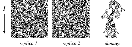
FIG. 1.: Temporal evolution of damage in the 1-$d$ Ising model of size $200$ with the dynamics of eq. (11) near the DS transition $J/k_{B}T^{*}$=0.2305. Each configuration is represented by a row of pixels and time goes downwards. The two replicas are started from identical initial conditions. At an early time, a damage of 5 sites is inserted in the center.

FIG. 2.: Numerical results for the 1-$d$ Ising model with A: the dynamics of eq. (11) and B: the dynamics of eq. (18). The measured quantities are explained in the text.

identical random initial conditions, where one damaged site is inserted at the center. Both replicas then evolve according to the dynamic rules of the system using the same set of random numbers. In order to minimize finite-size effects, we simulate a large system of $5000$ sites with periodic boundary conditions. For various temperatures we perform $10^{6}$ independent runs up to $1500$ time steps. However, in many runs damage heals very soon so that the run can be stopped earlier. As usual in this type of simulations, we measure the survival probability $P(t)$, the number of damaged sites $\Delta(t)$, and the mean-square spreading of damage from the center $R^{2}(t)$ averaged over the active runs. At the DS transition, these quantities are expected to scale algebraically in the large time limit:

$$P(t)\sim t^{-\delta}\,,\hskip 28.45274pt\Delta(t)\sim t^{\eta}\,,\hskip 28.45274ptR^{2}(t)\sim t^{z}\,.$$ (18)

The critical exponents $\delta,\eta,z$ are related to the density exponent $\beta$ and the scaling exponents $\nu_{\perp}$, $\nu_{||}$ by $\delta=\beta/\nu_{||}$, $z=2\nu_{\perp}/\nu_{||}$ and obey the hyperscaling relation $4\delta+2\eta=dz$. At criticality, the quantities (18) show straight lines in double logarithmic plots. Off criticality, these lines are curved. Using this criterion we estimate the critical temperature for the DS transition by $J/k_{B}T^{*}=0.2305(5)$. The exponents $\delta$, $\eta$, and $z$ are measured at criticality while the density exponent $\beta$ is determined off criticality by measuring the stationary Hamming distance $\Delta(T)\sim(T-T^{*})^{\beta}$ in the spreading phase. The results of our simulations are shown in Fig. 2. From the slopes in the double logarithmic plots we obtain the estimates $\delta=0.165(5)$, $\eta=0.315(10)$, $z=1.29(3)$, and $\beta=0.26(2)$ which are in fair agreement with the known [16] exponents for directed percolation $\delta=0.15947(3)$, $\eta=0.31368(4)$, $z=1.26523(4)$, and $\beta=0.27649(4)$. We therefore conclude that in agreement with Grassberger’s conjecture [8], the DS transition belongs to the DP universality class. This is very plausible; as far as the damage variable is concerned there is a single absorbing state (of no damage at all) and the transition is from a phase in which the system ends up in this state to one in which it does not, just as is the case for DP.

V Damage spreading transition with non-DP exponents

Different critical properties are expected [17, 18, 19, 20, 21, 22] for rules with two distinct absorbing states (of the damage variables!) related by symmetry. It is important to note that the $Z_{2}$ symmetry of the Ising system does not suffice - inverting all spins in both replicas does not change the damage variable (the Hamming distance between the two configurations). Therefore, we are looking for dynamic rules which (a) have two types of absorbing states; one with no damage and the other with full damage. Furthermore, (b) the two play completely symmetric roles. One can see that both (a) and (b) hold for rules that satisfy the condition

$$r_{\sigma_{i-1},\sigma_{i},\sigma_{i+1}}=-r_{-\sigma_{i-1},-\sigma_{i},-\sigma_{i+1}}\,.$$ (19)

The immediate consequence of this condition is that if a configuration $\{\sigma(t)\}$ evolves in one time step into $\{\sigma(t+1)\}$, then the spin-reversed configuration $\{-\sigma(t)\}$ will evolve into precisely $\{-\sigma(t+1)\}$. Imagine now simultaneous evolution of two replicas with initial states $\{\sigma\}$ and $\{\sigma^{\prime}\}$, giving rise to a damage field $\{\Delta\}$. Reversal of the initial state on one of the replicas will give sign-reversed spin states on this replica and hence the damage field $\{-\Delta\}$ will evolve. Thus, for rules that satisfy condition (16), the damage variable has an $Z_{2}$ symmetry. A particular consequence of this symmetry is that if two initial states are the exact sign-reversed of one another, this will persist at all subsequent times. Therefore, inasmuch as $\Delta=0$ (no damage) is an absorbing state, so is the situation of full damage, $\Delta=1$. For systems with such $Z_{2}$ symmetry we expect the DS transition (if it exists) to exhibit non-DP behavior.

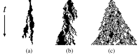
FIG. 3.: $Z_{2}$-symmetric damage spreading transition. Two replicas with 200 sites are started from identical random initial conditions. At an early time 5 damaged sites are introduced in the center. For fixed temperature $J/k_{B}T=0.25$ a typical temporal evolution of damage is shown for (a) Glauber dynamics $\lambda=1$, (b) near the transition $\lambda^{*}=0.82$ and (c) in the spreading regime $\lambda=0$. Because of the symmetry, islands of damaged sites can heal only at the edges.

It is quite remarkable to note that Glauber dynamics satisfies eq. (19)! The $Z_{2}$-symmetry of damage in the 1-$d$ Glauber model is illustrated in Fig. 3a. One can see that compact islands of damaged sites are formed because damage does not heal spontaneously inside such islands but only at the edges. However, as mentioned earlier, there is no DS transition in the 1-$d$ Glauber model.

Consider now a different dynamic rule:

$$r_{\sigma_{i-1},\sigma_{i},\sigma_{i+1}}=\left\{\begin{array}[]{ll}+{\rm sign}(p_{i}-z)&\mbox{if}\ \sigma_{i-1}\sigma_{i}\sigma_{i+1}=1\\ -{\rm sign}(1-p_{i}-z)&\mbox{if}\ \sigma_{i-1}\sigma_{i}\sigma_{i+1}=-1\end{array}\right.$$ (20)

For this rule, which also satisfies eq. (19), we observe in simulations that damage always spreads (see Fig. 3c). In order to generate an $Z_{2}$-symmetric DS transition in $1$-$d$, we use a rule that interpolates between this and Glauber. This can be done by introducing a second parameter $0\leq\lambda\leq 1$ and ‘switching’ between Glauber dynamics and rule (20) as follows: in each update an additional random number $\tilde{z}$ is generated. If $\tilde{z}\geq\lambda$, rule (20) is applied, otherwise Glauber dynamics is used. This mixed dynamics can be expressed as

$$r_{\sigma_{i-1},\sigma_{i},\sigma_{i+1}}=\left\{\begin{array}[]{ll}+{\rm sign}(p_{i}-z)&\mbox{if}\ y=1\\ -{\rm sign}(1-p_{i}-z)&\mbox{if}\ y=-1\\ \end{array}\right.\,,$$ (21)

where $y=\frac{1}{2}\sigma_{i}[(1+\sigma_{i-1}\sigma_{i+1})+(1-\sigma_{i-1}\sigma_{i+1}){\rm sign}(\lambda-\tilde{z})]$. Again this rule leads to the one-point correlations of eq.  (13), i.e., the temporal evolution of a single replica is the same as in Glauber and HB dynamics. However, varying $\lambda$ (at fixed T) we find a critical value $\lambda^{*}$ where a DS transition occurs. A typical temporal evolution of damage near the transition is shown in Fig. 3b.

Since ‘damage’ and ‘no damage’ play a symmetric role, the Hamming distance $\Delta$ (the density of damaged sites) cannot be used as an order parameter. Instead one has to use the density of kinks $N$ (domain walls) between damaged and healed domains. By definition, the number of kinks is conserved modulo two which establishes a parity conservation law. As can be seen in Fig. 3, two processes compete with each other: kinks annihilate mutually $(2X\rightarrow 0)$ and already existing kinks branch into an odd number of kinks ($X\rightarrow 3X,5X,\ldots$). Both processes resemble a branching annihilating walk with an even number of offspring. This branching process has a continuous phase transition that belongs to the so-called parity-conserving (PC) universality class. Phase transitions of this type have been observed in a variety of models, including certain probabilistic cellular automata [17], nonequilibrium kinetic Ising models with combined zero- and infinite-temperature dynamics [18], interacting monomer-dimer models [19], branching-annihilating random walks [20] and certain lattice models with two absorbing states [21]. In all these models the symmetry appears either as a parity conservation law or as an explicit $Z_{2}$-symmetry among different absorbing phases. A field theory describing PC transitions is currently developed in [22].

The PC universality class is characterized by the exponents $\delta=0.285(5)$, $\eta=0.00(1)$, $z=1.15(1)$, and $\beta=0.92(2)$. In fact, repeating the numerical simulations described above for $J/k_{B}T=0.25$ and $\lambda^{*}=0.82(1)$ (see Fig. 2), we obtain the estimates $\delta=0.295(10)$, $\eta=0.01(2)$, $z=1.17(3)$, and $\beta=0.86(5)$, which are in fair agreement with the known values. We therefore conclude that the DS transition observed for the dynamics of eq. (21) belongs to the PC universality class. Furthermore, our findings imply that the DS transitions observed [10] for the 2-$d$ Ising model with Glauber dynamics should also exhibit PC exponents (remember: $d=2$) in zero field, and cross over to (2-$d$) DP values when a field is switched on.

We thank D. Stauffer for sharing with us his knowledge of the DS literature and for encouragement. This work was supported by The Minerva Foundation and by the Germany-Israel Science Foundation (GIF).

REFERENCES

- [1] S.A. Kauffman, J. Theor. Biol. 22, 437 (1969).
- [2] P. Grassberger, Physica A 214, 547 (1995).
- [3] M. Creutz, Ann. Phys. 167, 62 (1986).
- [4] H. Stanley, D. Stauffer, J. Kertesz and H. Herrmann, Phys. Rev. Lett. 59, 2326 (1987).
- [5] B. Derrida and G. Weisbuch, Europhys. Lett. 4, 657 (1987).
- [6] A. M. Mariz, H. J. Herrmann and L. de Arcangelis, J. Stat. Phys. 59, 1043 (1990).
- [7] N. Jan and L. de Arcangelis, Ann. Rev. Comp. Phys. 1,1 (ed. D. Stauffer, World Scientific, Singapore 1994).
- [8] P. Grassberger, J. Stat. Phys. 79, 13 (1995).
- [9] H. Hinrichsen, S. Weitz, and E. Domany, preprint cond-mat/9611085, submitted to J. Stat. Phys.
- [10] P. Grassberger, J. Phys. A 28, L 67 (1995).
- [11] T. Vojta, preprint cond-mat/9610084 (1996).
- [12] U. M. S. Costa, J. Phys. A 20, L 583 (1987).
- [13] G. La Caer, J. Phys. A 22, L 647 (1989); Physica A 159, 329 (1989).
- [14] E. Domany and W. Kinzel, Phys. Rev. Lett. 53, 447 (1984).
- [15] P. Grassberger and A. de la Torre, Ann. Phys. (N.Y.) 122, 373 (1979).
- [16] I. Jensen, Phys. Rev. Lett. 77, 4988 (1996).
- [17] P. Grassberger, F. Krause, and T. von der Twer, J. Phys. A 17 L105 (1984); P. Grassberger, J. Phys. A 22, L1103 (1984).
- [18] N. Menyhárd, J. Phys. A 27, 6139 (1994); B. Menyhárd and G. Ódor, J. Phys. A 29, 7739 (1996). The kinetic Ising models introduced in these papers have mixed zero- and infinite-temperature dynamics and are different from the usual Ising model at finite temperature discussed in the present work.
- [19] H. H. Kim and H. Park, Phys. Rev. Lett. 73, 2579 (1994); H. Park, M. H. Kim, and H. Park, Phys. Rev. E 52, 5664 (1995).
- [20] I. Jensen, J. Phys. A 26 3921 (1993); D. ben-Avraham, F. Leyvraz, and S. Redner, Phys. Rev. E 50, 1843 (1994); I. Jensen, Phys. Rev. E 50 3623 (1994); D. Zhong and D. ben-Avraham, Phys. Lett. A 209, 333 (1995).
- [21] H. Hinrichsen, Phys. Rev. E 55, 219 (1997).
- [22] J. Cardy and U. C. Täuber, Phys. Rev. Lett. 77, 4780 (1996).