Geometrical consequences of foam equilibrium

Abstract

The equilibrium conditions impose nontrivial geometrical constraints on the configurations that a two-dimensional foam can attain. In the first place, the three centers of the films that converge to a vertex have to be on a line, i.e. all vertices are aligned. Moreover an equilibrated foam must admit a reciprocal figure. This means that it must be possible to find a set of points $P_{i}$ on the plane, one per bubble, such that the segments $\overline{P_{i}P_{j}}$ are normal to the corresponding foam films. It is furthermore shown that these constraints are equivalent to the requirement that the foam be a Sectional Multiplicative Voronoï Partition (SMVP). A SMVP is a cut with a two-dimensional plane, of a three-dimensional Multiplicative Voronoï Partition. Thus given an arbitrary equilibrated foam, we can always find point-like sources (one per bubble) in three dimensions that reproduce this foam as a generalized Voronoï partition. These sources are the only degrees of freedom that we need in oder to fully describe the foam.

I INTRODUCTION

Cellular structures[1, 2, 3, 4] appear in a wide range of natural phenomena, and have puzzled and fascinated scientists for decades[5]. They can be generally described as packings of space-filling cells of roughly polygonal shape, separated by thin interfaces to which a surface energy is associated. They arise as a consequence of competition between domains under the constraint of space-filling, and there is often some mechanism, such as the migration of a conserved quantity across the interface, which makes them evolve in time, i.e. coarsen.
Foams such as those obtained by shaking soapy water are the examples of cellular structures closest to our everyday experience. Two-dimensional foams may be obtained by confining a soap froth between two closely spaced glass plates. In spite of their apparent simplicity, foams display much of the phenomenology appearing in coarsening cellular structures. Foams have been the subject of interest since their relevance in the problem of grain growth was pointed out by Smith[6]. Despite the attention they have received, the understanding of their dynamical properties proved to be a tricky problem. Even some of the most basic issues, such as their asymptotic scaling properties, has been a matter of debate until recently (see references above). Numerically exact simulation procedures[7], as well as analytical[8] and numerical[9] approximations, have been useful in understanding the dynamics of ideal foams, but the system sizes accessible to available simulation procedures are strongly limited (for a complete account see refs.[3, 4]).
A satisfactory theoretical framework for the description of foams has not yet been achieved. The main result of this work consists in establishing a rigorous connection between foams and Voronoï partitions(VP). This connection provides a set of fundamental degrees of freedom for the foam (the source’s locations in space) and therefore constitutes a step towards the above mentioned theoretical understanding. On the other hand, an efficient method for the numerical simulation of ideal foams would also be highly desirable, and we propose that such a method could be obtained by exploiting the equivalence between foams and VP reported in this work. More precisely, we establish the following correspondence between equilibrated two-dimensional foams (EF) and a generalization of VPs, the Sectional Multiplicative Voronoï Partition (SMVP):
Given an arbitrary EF, it is always possible to find sources in space such that a SMVP with respect to them exactly gives this foam.
In Section II the VP and its generalizations are reviewed. The simplest generalizations of the VP concept are the Sectional Voronoï Partition and the Multiplicative Voronoï Partition. These correspond to adding a constant to the (square) distance and to multiplying it by a constant respectively. At the end of this section a combination of both is introduced, the Sectional Multiplicative Voronoï Partition. We will use this partition in order to describe foams.
The demonstration of the above mentioned correspondence between foams and SMVPs is divided in two parts (Sections III and IV) for clarity. In Section III, the recognition problem for SMVPs is solved. The recognition problem consists in giving the sufficient geometrical conditions that a circular partition has to satisfy in order to be a SMVP. We will see that if a circular partition has all of its vertices aligned and admits an oriented reciprocal figure, then it is a SMVP. In other words, it is always possible to find sources in three-dimensional space that give this circular partition as a SMVP. In this section we also describe the procedure to find the sources when these conditions are met. Some material that is needed in this section is described in the appendix.
Section IV deals with the equilibrium conditions for foams and its geometrical consequences. We start by writing the force and pressure equilibrium conditions in compact form in Section IV A. In Sections IV B and IV C it is shown that an equilibrated foam has all of its vertices aligned and admits an oriented reciprocal figure respectively. Therefore all equilibrated foams satisfy the conditions required in Section III, and can be described as SMVPs.
Finally in Section V the implications of this result are discussed, and some perspectives for future work are advanced.

II Space Partitions

A Voronoï Partition

Given a set of $N$ point-like sources $\{f_{i}\}$ in $n$-space, the Voronoï Partition (VP) or tessellation of space with respect to $\{f_{i}\}$ is a classification of space into cells $\Omega_{i}$ defined such that $x\in\Omega_{i}$ if $x$ is closer to $f_{i}$ than to any other source [10] .

$$\Omega_{i}=\{x\in R^{n}/\qquad d(x,i)<d(x,j)\quad\forall j\neq i\}$$ (1)

where $d(x,i)$ denotes the distance between $x$ and source $f_{i}$. This construction is also known under the names: Wigner-Seitz cells, Dirichlet Tessellations, Thiessen Polygons. In two dimensions, the dual lattice of a Voronoï partition is called Delaunay triangulation. Cell $\Omega_{i}$ can be seen as the “region of influence” of $f_{i}$, were the sources competing for some spatially distributed resource. It is common to use these constructions, and their generalizations, as approximate models for cellular structures occurring in nature[10, 11, 12, 22].
Two neighboring cells $\Omega_{i}$ and $\Omega_{j}$ are delimited by an interface $\Gamma_{ij}$ of points $x$ equidistant from $f_{i}$ and $f_{j}$.

$$\Gamma_{ij}=\{x\in R^{n}/\qquad d(x,i)=d(x,j)<d(x,k)\quad\forall k\neq i,j\}$$ (2)

These interfaces are $(n-1)$-dimensional hyperplanes normal to $\overline{f_{i}f_{j}}$. In two dimensions $\Omega_{i}$ are convex polygons and the interfaces $\Gamma_{ij}$ are straight lines (Fig. 1). Three interfaces $\Gamma_{ij}$, $\Gamma_{jk}$ and $\Gamma_{ki}$ meet at a vertex $v_{ijk}$, which is equidistant from $f_{i}$, $f_{j}$ and $f_{k}$. This means that $v_{ijk}$ is the center of a circle through $f_{i}$, $f_{j}$ and $f_{k}$. Vertices of higher multiplicity are possible for particular locations of the sources. For example a fourfold vertex would exist if four sources lay on the same circle. We will ignore the existence of these particular configurations, that is we will assume generic source locations. Under this assumption, all vertices are of multiplicity three.
The concept defining Voronoï partitions is equidistance. A simple way to generalize them is changing the way in which distances to the sources are measured. One lets each source measure the distance to points $x$ according to its own “rule”. The interface $\Gamma_{ij}$ is then the set of points $x$ for which two neighbors “claim” the same distance. Two simple ways to do this are: adding an arbitrary constant to the square of the distance (Sectional Voronoï partition [10, 13, 19]), and, multiplying the distance by a constant (Multiplicative Voronoï partition [10, 14, 19, 26]).

B Sectional Voronoï Partitions

A Sectional Voronoï Partition (SVP) is defined [10, 13, 19] as a $k$-dimensional cut of a higher dimensional Voronoï partition. The sources $\{P_{i}\}$ of the sectional partition are defined as the projections of the original sources $\{f_{i}\}$ onto this lower dimensional $k$-space. Cell $\Omega_{i}$ associated to source $P_{i}$ is the intersection of cell $\tilde{\Omega}_{i}$ (associated to $f_{i}$) with this $k$-dimensional hyperplane. For example, take sources $\{f_{i}\}$ in three dimensions (Fig. 2) and construct a VP with three-dimensional cells $\tilde{\Omega}_{i}$ and plane interfaces $\tilde{\Gamma}_{ij}$. Now project the sources $f_{i}=(x_{i},y_{i},z_{i})$ onto the $z=0$ plane (which we call the $\Pi_{z}$ plane) to obtain the projected sources $P_{i}=(x_{i},y_{i})$, which have associated “heights” $z_{i}$. Assign to each source $P_{i}$ the intersection $\Omega_{i}$ of $\tilde{\Omega}_{i}$ with $\Pi_{z}$. This defines the a sectional partition of $\Pi_{z}$ with respect to sources $\{P_{i}\}$ with heights $z_{i}$. Cells $\Omega_{i}$ are thus defined as

$$\Omega_{i}=\{x\in\Pi_{z}/\qquad d^{2}(x,i)+z_{i}^{2}<d^{2}(x,j)+z_{j}^{2}\quad\forall j\neq i\}$$ (3)

where $d(x,i)$ is the distance, on the $\Pi_{z}$ plane, between $P_{i}$ and point $x$.
In the same way, interfaces $\Gamma_{ij}$ are defined as

$$\Gamma_{ij}=\{x\in\Pi_{z}/\qquad d^{2}(x,i)+z_{i}^{2}=d^{2}(x,j)+z_{j}^{2}<d^{2}(x,k)+z_{k}^{2}\quad\forall k\neq i,j\}$$ (4)

Properties of these partitions in two dimensions are:

• Interfaces are straight lines and (generically) meet at triple vertices. ( In dimension $d$, vertices have multiplicity $d+1$).

• Interface $\Gamma_{ij}$ is normal to $\overline{P_{i}P_{j}}$, but not in general equidistant from $P_{i}$ and $P_{j}$.

• The partition is unchanged if all $z_{i}$ are changed according to: $z_{i}^{2}\to z_{i}^{2}+c^{2}$ for $c$ an arbitrary real.

An important difference with the Voronoï partition, is that in this case there may be sources to which no cell is associated. This happens if $\tilde{\Omega}_{i}$ is not cut by $\Pi_{z}$. It is easy to see that SVPs are equivalent to Laguerre Partitions [13].
Appendix A discusses the recognition problem for this kind of partitions, that is giving the sufficient conditions for an arbitrary rectilinear partition to be a SVP. We will use similar concepts in Section III in order to solve the recognition problem for Sectional Multiplicative Voronoï Partitions.
As an example of the application of sectional partitions, consider the case of sources $f_{i}$ whose location in space changes in time, giving rise to a time-dependent partition of $\Pi_{z}$. If for example source $f_{1}$ moves away from $\Pi_{z}$, the two-dimensional cell $\Omega_{1}$ will shrink and finally disappear when $\tilde{\Omega}_{1}$ no longer cuts $\Pi_{z}$. Therefore the number of cells can vary without changing the number of sources. Thus sectional partitions can be used as dynamical models for crystal growth [22], and other processes in which some cells disappear or are created.

C Multiplicative Voronoï Partition

The Multiplicative Voronoï Partition (MVP) [14, 19, 26] is defined by assigning to each source $f_{i}$ a positive intensity $a_{i}$, and defining the multiplicative distance $d_{m}(x,i)=d(x,i)/a_{i}$. The cell $\Omega_{i}$ associated to source $f_{i}$ is then the set of points $x$ closer to $f_{i}$ (in terms of this multiplicative distance) than to any other source

$$\Omega_{i}=\{x\in R^{n}/\qquad{d(x,i)\over a_{i}}<{d(x,j)\over a_{j}}\quad\forall j\neq i\}$$ (5)

Interfaces $\Gamma_{ij}$ are hyperspherical surfaces (circle arcs in two dimensions) satisfying

$$\Gamma_{ij}=\{x\in R^{n}/\qquad{d(x,i)\over a_{i}}={d(x,j)\over a_{j}}<{d(x,k)\over a_{k}}\quad\forall k\neq i,j\}$$ (6)

In two dimensions, the circular interface of a MVP with two sources is one of the Apollonius circles (see for example [24]) of those two points. In arbitrary dimensions let $d_{ij}$ be the distance between two sources $f_{i}$ and $f_{j}$, and $A_{ij}=a_{j}/a_{i}$. Without loss of generality we take $A_{ij}<1$. This means that $f_{j}$ has the smallest intensity and therefore $\Omega_{j}$ will be the interior of a hypersphere, while $\Omega_{i}$ will be its exterior. The following properties are satisfied in any dimension.

• $f_{i}$ is contained in $\Omega_{i}$.

• $\Gamma_{ij}$ has radius $R_{ij}=A_{ij}d_{ij}/(1-A_{ij}^{2})$, and its center $C_{ij}$ is on the straight line going through $f_{i}$ and $f_{j}$.

• $C_{ij}$ is located at a distance $d_{ij}/(1-A_{ij}^{2})$ from $f_{i}$, that is, it never lays between $f_{i}$ and $f_{j}$.

Three sources give rise to a tessellation like the one shown in Fig. 3. The exterior of the two “bubbles” is the infinite cell associated to the source with the largest intensity, $f_{1}$ in this example. For some choices of $\{a_{i}\}$ the interfaces will not intersect. In this case the tessellation is simply a pair of circles, each containing one of the sources with smaller intensities, while the exterior of these two circles is the cell of the source with larger intensity. MVPs can be interpreted again as “areas of influence” of sources $f_{i}$, but now each source has a different strength.
Consider a MVP of two dimensional space with respect to a set of sources $\{f_{i}\}$. If three interfaces $\Gamma_{ij}$, $\Gamma_{jk}$ and $\Gamma_{ki}$ meet at a vertex (again, vertices of higher multiplicity are only possible for particular configurations, which we ignore here), then centers $C_{ij}$, $C_{jk}$ and $C_{ki}$ lay on a line. The reason why this is so is simple. If two interfaces $\Gamma_{ij}$ and $\Gamma_{jk}$ have a common point $v_{ijk}$ , then their continuations must meet again at another point $v^{*}_{ijk}$, the conjugate vertex. But then the third interface $\Gamma_{ik}$ must also go through this point since $d(v^{*},i)/a_{i}=d(v^{*},j)/a_{j}$ and $d(v^{*},j)/a_{j}=d(v^{*},k)/a_{k}$ implies $d(v^{*},i)/a_{i}=d(v^{*},k)/a_{k}$. Therefore two points exist ($v$ and $v^{*}$) at which all three circles intersect. Then the centers of these circles must be on a line (Fig. 3).
Let us define a Circular Partition(CP) of two-dimensional space to be a classification of space in cells delimited by arbitrary circle arcs that meet at triple points called vertices. No three centers of these arbitrarily defined interfaces will in general be on a line. We will say that a vertex of a CP is aligned if the centers of the three interfaces defining it are on a line. As we saw, all vertices of a MVP are aligned in 2d. Therefore for each triple vertex of a MVP in 2d, the three sources and the three centers form the configuration [25] $(6_{2},4_{3})$ of projective geometry. Since $C_{ij}$ cannot be between $P_{i}$ and $P_{j}$, the three centers can only be on one of the two external segments of the configuration.
In a three-dimensional MVP, four cells meet at each vertex $v_{ijkl}$, giving rise to six spherical interfaces $(ij),(ik),(il),(jk),(jl),(kl)$. The centers of these interfaces are aligned in triplets so that the six centers also form the configuration $(6_{2},4_{3})$, this time in three-dimensional space. This has the implication that the six centers are necessarily on the same plane.
The MVP was first introduced by Boots [14] to describe areas of influence in geography. Ash and Bolker [19] also studied the recognition problem, that is, under which conditions a CP is a MVP. The visual similarity between this kind of partitions and two-dimensional foams is striking, and suggests the idea to find a connection between them. Obviously the centers of the films of a foam must be aligned for each triple vertex, if the foam is to be described as a MVP, since MVPs are aligned. One finds [26] that this alignment condition is indeed satisfied by all vertices of arbitrary equilibrated foams. Despite this (which is a necessary but not sufficient condition for a foam to be a MVP), two-dimensional MVPs cannot describe all possible equilibrated foams in two dimensions. This work shows the reason of this limitation: In order to describe arbitrary equilibrated two-dimensional foams we must introduce the sectional variant of a multiplicative partition. In other words, instead of confining the sources to the plane, we let them exist in a three-dimensional space and obtain the foam as a two-dimensional cut of a three-dimensional MVP.

D Sectional Multiplicative Voronoï Partition

We will restrict the description to the case of a plane cut of a three dimensional MVP. The generalization to a $k$-dimensional cut of an $n$-dimensional MVP is straightforward.
A plane cut, with a plane $\Pi_{x}$, of a three-dimensional MVP defines a Sectional Multiplicative Voronoï Partition (SMVP) of $\Pi_{z}$ (See Figs. 4 and 5). The sources $P_{i}$ of this SMVP are the normal projections onto $\Pi_{z}$ of the original sources $f_{i}$, and may be seen to have as attributes both an intensity $a_{i}$ and a height $z_{i}$. Cells $\Omega_{i}$ associated to sources $P_{i}$ are defined as

$$\Omega_{i}=\{x\in\Pi_{z}/\qquad{d(x,i)^{2}+z_{i}^{2}\over a_{i}^{2}}<{d(x,j)^{2}+z_{j}^{2}\over a_{j}^{2}}\quad\forall j\neq i\}$$ (7)

In the same way, interfaces $\Gamma_{ij}$ are circle arcs satisfying

$$\Gamma_{ij}=\{x\in\Pi_{z}/\qquad{d^{2}(x,i)+z_{i}^{2}\over a_{i}^{2}}={d^{2}(x,j)+z_{j}^{2}\over a_{j}^{2}}<{d^{2}(x,k)+z_{k}^{2}\over a_{k}^{2}}\qquad\forall k\neq i,j\}$$ (8)

An example of a SMVP with three sources is shown in Figs. 4 and 5. We see that there are two vertices on $\Pi_{z}$ at which the three interfaces meet. In a general case (for example in a partition with respect to many sources like in Fig. 6), if vertex $v_{ijk}$ exists, then the continuations of interfaces $\Gamma_{ij}$, $\Gamma_{jk}$ and $\Gamma_{ki}$ meet at a conjugate vertex $v^{*}_{ijk}$ also. This implies the alignment of centers $C_{ij}$, $C_{jk}$ and $C_{ki}$, which could also be deduced from the alignment of $E_{ij}$, $E_{jk}$ and $E_{ki}$ in three-dimensions (Fig. 4) .
We notice that the SMVP is equivalent to a Multiplicative Laguerre Partition, since a SVP is equivalent to a Laguerre Partition [13]. As is usual in sectional partitions, in the SMVP there may be sources $P_{i}$ with no associated cell, those for which the corresponding three-dimensional “bubble” $\tilde{\Omega}_{i}$ does not cut $\Pi_{z}$.
It was seen in section II C that the spherical interface $\tilde{\Gamma}_{ij}$ in three dimensions is cut normally by the segment $\overline{f_{i}f_{j}}$. As a projective consequence of this, the straight line containing $P_{i}$ and $P_{j}$ on $\Pi_{z}$ is normal to the circular interface $\Gamma_{ij}$. In other words, $P_{i}$, $P_{j}$ and $C_{ij}$ are on the same line. Furthermore and since $E_{ij}$ never lays between $f_{i}$ and $f_{j}$ in 3d, we notice that $C_{ij}$ is always outside the segment $\overline{P_{i}P_{j}}$.

III When a Circular Partition is a SMVP

In this section the sufficient conditions for a CP to be a SMVP are given. We first introduce the notion of oriented reciprocal figure for CPs, and then proceed to demonstrate that an aligned CP admitting such a reciprocal figure is a SMVP.

A Reciprocal figure of a circular partition

We will now generalize the concept of reciprocal figure as appropriate for circular partitions. We say that a graph $\cal R$ made of points $P_{i}$ connected by edges $(ij)$ forms a reciprocal figure for a CP $\cal P$ if,

• points $P_{i}$ are in correspondence with the cells $\Omega_{i}$ of $\cal P$.

• edges $(ij)$ are in correspondence with the interfaces $\Gamma_{ij}$ of $\cal P$.

• for each $\Gamma_{ij}$ in $\cal P$, points $P_{i}$, $P_{j}$ and $C_{ij}$ lay on the same line.

Consider two regions $\Omega_{i}$ and $\Omega_{j}$ separated by a circular interface $\Gamma_{ij}$. A reciprocal figure $\cal R$ will be said to respect orientation if for each $\Gamma_{ij}$ in $\cal P$:

• $C_{ij}$ is not between $P_{i}$ and $P_{j}$.

• starting from $C_{ij}$ and traveling along $\overline{C_{ij}P_{i}P_{j}}$ to infinity, points $P_{i}$ and $P_{j}$ are found in the same order as regions $\Omega_{i}$ and $\Omega_{j}$ are.

We saw already that all SMVPs are aligned (all vertices satisfy the alignment condition introduced in Sec. II C). On the other hand, it is clear that the sources $P_{i}$ of a SMVP form a reciprocal figure that satisfies orientation. Therefore

$$\cal P\hbox{ is a SMVP }\Rightarrow\cal P\hbox{ is aligned and admits an oriented reciprocal figure}$$

Figure 7 shows four possible partitions that share the same centers $C_{12}$, $C_{23}$ and $C_{31}$. All four admit reciprocal figures. But only in cases a) and c) a reciprocal figure that satisfies orientation can be constructed. Therefore neither b) nor c) can be a SMVP. The reason is that the orientation condition cannot be satisfied if any of the vertices is not convex. A vertex is convex if all the internal angles formed by the interfaces are less than $\pi$. Convexity of all vertices is clearly a necessary condition for a circular partition to be a SMVP.
We are now ready to give the sufficient conditions for a circular partition to be a SMVP. We will show in Section III B that if a circular partition $\cal P$ is aligned and admits a reciprocal figure that satisfies orientation, then it is a SMVP.

$$\cal P\hbox{ is aligned and admits an oriented reciprocal figure}\Rightarrow\cal P\hbox{ is a SMVP}$$

B Finding the sources of a SMVP.

Given a circular partition $\cal P$ of a region of two dimensional space, all whose (triple) vertices are aligned, we show here that, if $\cal P$ admits a reciprocal figure that satisfies orientation, then $\cal P$ is a SMVP with respect to sources $f_{i}$ located somewhere above points $P_{i}$. Our demonstration is constructive, that is we explicitly show how the sources and intensities are determined. We will use for this purpose the inversion transformation (Appendix B) to straighten each vertex in turn, that is, transform a circular vertex into a rectilinear one. This rectilinear vertex is one of a of a SVP. Sources are located in this straight representation (Appendix A), and then transformed back to the original system. The intensities $a_{i}$ of the corresponding SMVP are obtained in this back-transformation, since the SMVP is invariant under inversion.
Let $v$ be an aligned vertex on which three interfaces $\{\Gamma_{12},\Gamma_{23},\Gamma_{32}\}$ meet, and $\{P_{1},P_{2},P_{3}\}$ the three points of the reciprocal figure associated to the three bubbles sharing the vertex, as in Fig. 8. The conjugate vertex $v^{*}$ is obtained as the intersection point of the continuations of the interfaces, which happens at a unique point because of alignment. Let furthermore $\lambda_{i}$ be the straight line through $v^{*}$ and $P_{i}$. We start by showing that

Theorem 1

A monoparametric family of triplets of circles $\{\omega_{12},\omega_{23},\omega_{31}\}$ exists, which has the following properties:

• $\omega_{12}$, $\omega_{23}$ and $\omega_{31}$ intercept each other on $v^{*}$.

• $\omega_{ij}\perp\Gamma_{ij}$.

• The intersection point $q_{i}$ between $\omega_{ij}$ and $\omega_{ik}$ lays on $\lambda_{i}$.

The non-trivial content of the theorem is the fact that the three intersection points $q_{i}$ of these normal circles $\omega_{ij}$ lay on the lines $\lambda_{i}$. For example take an arbitrary point $q_{1}$ on $\lambda_{1}$ and draw a circle $\omega_{12}$ through $q_{1}$, $v^{*}$ and normal to $\Gamma_{12}$. Let $q_{2}$ be the intersection of $\omega_{12}$ with $\lambda_{2}$. Draw now a circle $\omega_{23}$ trough $q_{2}$, $v^{*}$ and normal to $\Gamma_{23}$. Let $q_{3}$ be its intersection with $\lambda_{3}$. Then the circle $\omega_{31}$ through $v^{*}$, $q_{1}$ and $q_{3}$ is normal to $\Gamma_{13}$.
Proof. The demonstration is done by first performing an inversion with center $v^{*}$ and arbitrary radius, whereupon the interfaces $\Gamma_{ij}$ are transformed into straight lines $\Gamma_{ij}^{\prime}$ meeting at $v^{\prime}$ (Fig. 9). This transformed system will be referred to as the “straight” representation of that vertex. Primed names are used in the straight representation, with the exception of $v^{*}$, whose original location is kept in Fig. 9 ($v^{*}$ itself is mapped to $\infty$ by the inversion). Lines originally not going through $v^{*}$ are transformed into circles through $v^{*}$, as is the case of $\{S_{12},S_{23},S_{31}\}$, which form the reciprocal figure in the original system. Circles $\omega_{ij}$ are transformed into straight lines $\omega_{ij}^{\prime}$ going through $q_{i}^{\prime}$ and $q_{j}^{\prime}$, respectively on $\lambda_{i}$ and $\lambda_{j}$, which are invariant.
The inversion transformation preserves angles, therefore circle $S_{ij}^{\prime}$ is normal to the now straight interface $\Gamma_{ij}^{\prime}$. This means that its center $L_{ij}$ must lay on $\Gamma_{ij}^{\prime}$. Consider the figure formed by $v^{\prime}$, $L_{12}$, $L_{23}$ and $L_{31}$, and the six lines joining them. Maxwell [17] showed that a figure made of four points joined by six lines always has a reciprocal figure (to see this just consider the centers of the four circles going through three of these points). We will now identify it on Fig. 9 as the figure formed by $v^{*}$, $q^{\prime}_{1}$, $q^{\prime}_{2}$ and $q^{\prime}_{3}$. First we notice that circles $S_{ij}^{\prime}$ and $S_{jk}^{\prime}$ intercept each other at two points $v^{*}$ and $P_{j}^{\prime}$, both on $\lambda_{j}$. Therefore lines $\overline{L_{ij}L_{jk}}$ are normal to $\lambda_{j}$, and we have identified the first three lines of the reciprocal figure. The other three lines $\omega_{ij}=\overline{q_{i}^{\prime}q_{j}^{\prime}}$ of the reciprocal figure have to be normal to the segments $\overline{vL_{ij}}$, so they are normal to the interfaces $\Gamma_{ij}^{\prime}$. Since the inversion preserves angles, this means that $\omega_{ij}\perp\Gamma_{ij}$ in the original system (Fig. 8). $\diamond$
We see that the existence of triplets of circles $\{\omega_{12},\omega_{23},\omega_{31}\}$ with the above mentioned properties is a consequence of the existence, in the straight representation, of a figure $v^{*}q_{1}^{\prime}q_{2}^{\prime}q_{3}^{\prime}$, which is the reciprocal of $vL_{12}L_{23}L_{31}$. In other words, Theorem 1 means that in the straight representation, triangle $q_{1}^{\prime}q_{2}^{\prime}q_{3}^{\prime}$ forms a reciprocal figure for the rectilinear vertex. Clearly this reciprocal figure $q_{1}^{\prime}q_{2}^{\prime}q_{3}^{\prime}$ satisfies orientation if the original figure $P_{1}P_{2}P_{3}$ satisfies orientation in the circular system. Therefore as discussed in Appendix A, it is always possible to find three sources $f_{i}^{\prime},\quad i=1,2,3$, located at heights $z_{i}^{\prime}$ above points $q_{i}^{\prime}$, such that this rectilinear vertex is a SVP with respect to them. Once these sources $f_{i}^{\prime}$ are known in the straight representation, a second inversion around the same point $v^{*}$ takes us back to the original system and provides the original locations $f_{i}$ of the sources.
If $v_{123}$ is the first vertex to be considered in the system, we have one degree of freedom in the determination of the circles $\omega_{ij}$, or equivalently of points $q_{i}$. Once in the straight representation, there is one more degree of freedom: the determination of one of the heights $z_{i}^{\prime}$. We will now show that, if this $z_{i}^{\prime}$ is chosen appropriately, the three back-transformed sources $f_{i}$ are located above their respective points $P_{i}$.
Consider a plane $\Pi_{i}$ that is normal to $\Pi_{z}$ and contains $\lambda_{i}$, as shown in Fig. 10. Draw a circle $\beta_{i}$ through $q_{i}$, $v^{*}$ and normal to $\Pi_{z}$. Let $u_{i}$ be the intersection of this circle with the normal $\alpha_{i}$ to $\Pi_{z}$ through $P_{i}$. Now under an inversion with center $v^{*}$, point $u_{i}^{\prime}$ is above $q_{i}^{\prime}$, since circle $\beta_{i}$ is transformed in a straight line $\beta_{i}^{\prime}$, normal to $\Pi_{z}$. Straight line $\alpha_{i}$ normal to $\Pi_{z}$ through $P_{i}$ is now a circle $\alpha_{i}^{\prime}$ through $v^{*}$, $u_{i}^{\prime}$ and normal to $\Pi_{z}$. Its intersection with $\Pi_{z}$ determines the image $P_{i}^{\prime}$. Now we now that source $f_{i}^{\prime}$ is located somewhere on $\beta_{i}^{\prime}$. The sources can be displaced vertically (simultaneously) according according to what we saw in Appendix A, but not independently. Fixing the height $z_{i}^{\prime}$ of one of them determines the other two uniquely. What we want to demonstrate is that if one of the sources $f_{i}^{\prime}$ coincides with its point $u_{i}^{\prime}$, then the other two also do. In order to do this, take for example the sphere $\tilde{\cal X}_{12}$ through $v^{*}$, $f_{1}^{\prime}$, $f_{2}^{\prime}$ and normal to $\Pi_{z}$. In the straight representation, interface $\tilde{\Gamma}_{12}^{\prime}$ of the Voronoï Partition with respect to sources $f_{1}^{\prime}$ and $f_{2}^{\prime}$ is a plane, equidistant from $f_{1}^{\prime}$ and $f_{2}^{\prime}$, and normal to $\overline{f_{1}^{\prime}f_{2}^{\prime}}$. This means that $\tilde{\Gamma}_{12}^{\prime}$ is normal to $\tilde{\cal X}_{12}$. As a consequence, the intersection ${\cal X}_{12}$(a circle) of $\tilde{\cal X}_{12}$ with $\Pi_{z}$ is normal to the intersection $\Gamma_{12}^{\prime}$(a straight line) of $\tilde{\Gamma}_{12}^{\prime}$ with $\Pi_{z}$. Now assume that $f_{1}^{\prime}=u_{1}^{\prime}$. This means that $P_{1}^{\prime}\in\tilde{\cal X}_{12}$ since $\alpha_{1}^{\prime}$ is in this case contained in $\tilde{\cal X}_{12}$. But then the circle ${\cal X}_{12}$ is the circle $S_{12}^{\prime}$ (Fig. 9) that goes through $P_{1}^{\prime}$, $P_{2}^{\prime}$ and $v^{*}$ and is normal to $\Gamma_{12}^{\prime}$. This implies that $P_{2}^{\prime}$ is also in $\tilde{\cal X}_{12}$, which in turn implies $f_{2}^{\prime}=u_{2}^{\prime}$. The same reasoning can be repeated for the pair of sources $1$ and $3$.
We have thus shown that all sources $f_{i}$ are, in the back-transformed, original system, located above the points $P_{i}$ of the reciprocal figure. In other words, that the given reciprocal figure is the projection of the sources $f_{i}$ on the $\Pi_{z}$ plane.
Now we have to determine the heights $z_{i}$ and intensities $a_{i}$. The heights $z_{i}$ of the sources can be found found by back-transforming the sources $f_{i}^{\prime}$ from the straight system. But in practice this is not necessary. By looking at Fig. 10 we notice that triangle $v^{*}f_{i}q_{i}$ is rectangle. Therefore

$$z_{i}^{2}=|v^{*}P_{i}|\times|P_{i}q_{i}|,$$ (9)

which suffices to locate the sources $f_{i}$ with the sole knowledge of points $P_{i}$ and $q_{i}$ in the original system. Knowing now the spatial locations of the sources $f_{i}$ in three dimensions, the intensities $a_{i}$ follow immediately since the vertex $v^{*}$ is equidistant [29] from the three sources. This means

$$a_{i}=A|v^{*}f_{i}|=A(|v^{*}P_{i}|\times|v^{*}q_{i}|)^{1/2}$$ (10)

Here $A$ is an arbitrary positive constant. Alternatively we can get the same result by using the transformation properties (eq. B2) of the $a_{i}$’s and the fact that the intensities are all equal in the straight system.
We have used the inversion transformation to demonstrate that the given vertex is a SMVP with respect to sources $f_{i}$ located above $P_{i}$, and showed how the sources $f_{i}$ can be located without the need to explicitly perform an inversion for each vertex. All we need is to know the location of points $q_{i}$, which we are free to choose for the first vertex under consideration. This first choice determines all subsequent $q_{i}$ points, and therefore all sources. It is clear from Fig. 10 that $|v^{*}q_{i}|\geq|v^{*}P_{i}|$ has to be satisfied. Therefore one has to choose the triplet of circles $w_{ij}$ such that this condition is verified for the three points $q_{i}$. If one of the $q_{i}$ coincides with $P_{i}$, this means that the corresponding height $z_{i}$ is zero, i.e. the source $f_{i}$ lays on the $\Pi_{z}$ plane. A point $q_{i}$ closer to $v^{*}$ than the corresponding $P_{i}$ is not acceptable.
The general procedure to determine the sources can now be described. Assume we are given a circular tessellation which satisfies the required conditions of alignment and convexity, and that we are able to find, or are given, a reciprocal figure $P_{i}$ for it. We start from one of the cells of the partition, as in Fig. 11. Take an arbitrary vertex to start with, for example vertex $v_{012}$, and determine tentative locations for point $q_{0}$ on $\lambda_{0}$. This fixes $q_{1}$ and $q_{2}$ as discussed in Section III B. After fixing $q_{0}$ the rest of the construction is uniquely determined. The locations $q_{0},q_{1},q_{2}$ determine $z_{0},z_{1}$ and $z_{2}$, and the corresponding intensities $a_{0},a_{1}$ and $a_{2}$, through equations (9) and (10). Now proceed to the neighboring vertex $v_{023}$. Two of the sources, $f_{0}$ and $f_{2}$ are already known, only the height $z_{3}$ of $f_{3}$ has to be found. First one has to find the new locations of $q_{0}$ and $q_{2}$ when defined from vertex $v_{023}^{*}$. In order to do this, lines $\lambda^{023}_{i}$ from vertex $v_{023}^{*}$ are drawn, and $q_{0}$ and $q_{2}$ are located using the fact that the heights $z_{0}$ and $z_{2}$ are already known. Equation (9) implies

$$|P_{0}q_{0}^{(023)}|=|P_{0}q_{0}^{(012)}|{|v^{*}_{(012)}P_{0}|\over|v^{*}_{(023)}P_{0}|}$$ (12)

$$|P_{2}q_{2}^{(023)}|=|P_{2}q_{2}^{(012)}|{|v^{*}_{(012)}P_{2}|\over|v^{*}_{(023)}P_{2}|}$$ (13)

Once the new $q_{0}$ and $q_{2}$ are known, the next step is to draw circles $\omega_{03}$ and $\omega_{23}$ through them and normal to the respective interfaces. Their intersection gives the location of $q_{3}$ (this intersection always occurs on $\lambda_{3}^{023}$, as Theorem 1 shows). This determines $z_{3}$ and $a_{3}$ using equations (9) and (10). This procedure of triangulation is repeated until all sources are located. Eventually it may happen that a point $q_{i}$ is found to be closer to the conjugate vertex $v^{*}$ than the corresponding $P_{i}$. This is not acceptable and means that the tentative starting position of $q_{0}$ has to be changed. It must be shifted away from $v_{012}^{*}$ and the whole procedure repeated. It is easy to see that taking a large enough value of $q_{0}$ always solves this problem.
One could ask whether this construction can be closed self-consistently. For example after determining $f_{5}$ from $f_{0}$ and $f_{4}$ in our example of Fig. 11, one can go on with the procedure as if $f_{1}$ were unknown. Would the position of $f_{1}$ determined by $f_{0}$ and $f_{5}$ be the same one as found initially? Alternatively: if we used $f_{0}$ and $f_{1}$ to determine $f_{5}$ instead of going around the bubble in the opposite sense, would its position be the same as found after going around the bubble? The answer is yes because of unicity. As discussed in Appendix A, the height of one of the sources of a vertex determines the other two uniquely. This means that $f_{1},f_{2},\cdots,f_{5}$ are all uniquely determined by $f_{0}$.

IV Equilibrated Foams.

In this section we show that a two dimensional foam in equilibrium satisfies all conditions required for it to be a SMVP. In order to do this let us first write down the equilibrium conditions for an arbitrary vertex of the foam, in compact form. We will consider the case of foams with arbitrary surface tensions, and also allow forces to act on the foam’s vertices.

A Equilibrium equations

Let $\vec{v}$ be the location of a vertex $v$ at which three interfaces $\Gamma_{1}$, $\Gamma_{2}$ and $\Gamma_{3}$ meet, as shown in Fig. 12. Each interface $\Gamma_{i}$ is a circle arc with radius $r_{i}$ and center $\vec{C}_{i}$. It produces on $v$, due to its surface tension $\tau_{i}$, a force $\vec{T}_{i}$ of modulus $2\tau_{i}$ in the direction of the tangent to the film at $\vec{v}$. These forces $\vec{T}_{i}$ can therefore be written as

$$\vec{T}_{i}=-2{\tau_{i}\over r_{i}}\vec{K}_{i}^{*}=-\xi_{i}\vec{K}_{i}^{*},$$ (14)

where $\vec{K}_{i}=\vec{C}_{i}-\vec{v}$ and $\xi_{i}=2\tau_{i}/r_{i}$. The asterisk stands here for a counterclockwise rotation in $\pi/2$, so that ${\vec{e}_{x}}^{*}=\vec{e}_{y}$.
Let us more generally assume that an external force $\vec{F}$ acts on $v$. Equilibrium of all forces acting on the vertex implies

$$\vec{F}^{*}+\sum_{i=1}^{3}\xi_{i}\vec{K}_{i}=0\qquad\qquad i=1,2,3$$ (15)

There is still one more condition, which is related to pressure equilibrium around the vertex. The pressure drop across an interface can be written as

$$\Delta p_{i}=2{\tau_{i}\over r_{i}}=\xi_{i}$$ (16)

We will adopt the convention for $\Delta p$ to be positive if the pressure decreases when crossing the interface in the counterclockwise sense of rotation around $v$. This is of course related to a convention for the signs of the $r_{i}$. In Fig. 12 $r_{1}$ and $\Delta p_{1}$ are negative according to this convention. Notice that pressure jumps and radii have different signs when considered from the two opposite vertices joined by a film.
The fact that the total accumulated pressure drop around a vertex has to be zero implies then

$$\sum_{i=1}^{3}\xi_{i}=0.$$ (17)

This is the pressure equilibrium condition for the vertex. Equations (15) and (17) are satisfied if the vertex is equilibrated, and are together equivalent to

$$\vec{F}^{*}+\sum_{i=1}^{3}\xi_{i}(\vec{C}_{i}-\vec{x})=0,$$ (18)

where $\vec{x}$ is an arbitrary point. This is what we will call the equilibrium condition for the vertex, and encloses both force and pressure equilibrium.

B Equilibrium implies alignement

The alignment of the centers of a two-dimensional foam was already known long time ago by Plateau [15] for equal surface tensions, and in the case of small self-standing clusters of 2 and 3 bubbles. For the case of a cluster of two bubbles and zero load it is a trivial consequence of symmetry [16]. The demonstration for the case of clusters of three bubbles is referred to by Boys as being“rather long and difficult” [15].
It is not difficult to see that the alignment of the centers is in no way a property of clusters, and also not restricted to vertices with equal surface tensions and zero loads, but a general consequence of equilibrium. We will find that under very general conditions such as arbitrary surface tensions and external loads applied on the vertices, if a vertex is equilibrated then the centers of the three arcs converging to it lay on a line.
Consider equation (18), and assume for a moment that the external load is zero. Then $C_{1},C_{2}$ and $C_{3}$ lay on the same line, as can be seen by taking $\vec{x}=\vec{C}_{1}$ for example. Thus all vertices in equilibrium are aligned if no external force is applied on it. This alignment property is even true under non-zero load conditions, if the force is perpendicular to the line of centers. A load satisfying such condition will be called a normal load. The alignment condition has the geometrical consequence that the interfaces $\Gamma_{i}$, when continued, meet each other again at a unique point $v^{*}$ which we called the conjugate vertex [23] of $v$. This also means that the vertex $v$ could be physically realized as a self-standing cluster of two bubbles (by continuing its interfaces), and is a kind of a “separability” condition for the static equilibrium conditions, in the sense that each vertex of a foam might as well be that of an isolated cluster of two bubbles. Thus

A vertex in equilibrium under a normal load is aligned.

or ,equivalently

A vertex in equilibrium under a normal load has a conjugate vertex.

Next we would like to consider the existence of a reciprocal figure, since this is also a condition that has to be satisfied in order for a foam to be a SMVP. This condition must be separately considered. The reader may easily build examples of bubbles with $n$ neighbors, all of whose $n$ vertices are aligned, but yet do not admit a reciprocal figure. The reason is that the attempted reciprocal figure will not in general “close” around that bubble, the same case as described in Appendix A.

C Equilibrium implies Reciprocal Figure

We will now show that if all vertices of a foam are equilibrated, then an oriented reciprocal figure exists for it. We start by considering a bubble and show that the reciprocal figure can be found for it. The figure for the whole foam can then be formed by patching together those of neighboring bubbles. Consider a bubble with $n$ neighbors $\alpha=1,2,\cdots,n$, as shown in figure 13. At each vertex $v_{\alpha}$ of this bubble, three films $\Gamma_{\alpha}$, $\Gamma_{\alpha+1}$ and $\Gamma_{\alpha}^{\alpha+1}$ meet. Interface $\Gamma_{\alpha}$ separates the central bubble from its neighbor $\alpha$, while interface $\Gamma_{\alpha}^{\alpha+1}$ is the limit between neighbors $\alpha$ and $(\alpha+1)$. We will assume vertices $v_{\alpha}$ to be in equilibrium under arbitrary normal loads $\vec{F}_{\alpha}$. These loads we can generally write as

$$\vec{F}_{\alpha}^{*}=-R_{\alpha+1}\vec{C}_{\alpha+1}+S_{\alpha}\vec{C}_{\alpha}+T_{\alpha}\vec{C}_{\alpha}^{\alpha+1}$$ (19)

That is, we have decomposed the external load of vertex $v_{\alpha}$ in the dependent basis formed by the three centers of the films meeting at the vertex. Because these centers are aligned, and the load is normal to the line of centers, the following condition is always satisfied by the coefficients.

$$-R_{\alpha+1}+S_{\alpha}+T_{\alpha}=0.$$ (20)

The equilibrium condition (18) now reads

$$-(\xi_{\alpha+1}+R_{\alpha+1})(\vec{C}_{\alpha+1}-\vec{x}_{\alpha})+(\xi_{\alpha}+S_{\alpha})(\vec{C}_{\alpha}-\vec{x}_{\alpha})+(\xi_{\alpha}^{\alpha+1}+T_{\alpha})(\vec{C}_{\alpha}^{\alpha+1}-\vec{x}_{\alpha})=0,\qquad\alpha=1,\cdots n$$ (21)

and holds for arbitrary $x_{\alpha}$’s. The sign of $\xi_{\alpha}$ is determined by the sign convention at vertex $v_{\alpha}$, therefore $\xi_{\alpha+1}$ must appear with a minus sign in the equilibrium equation for vertex $\alpha$.
Since we use a dependent basis (equation. (19)) the coefficients $\{R_{\alpha+1},S_{\alpha},T_{\alpha}\}$ (the “representation” of the load) are not uniquely determined for a given load. There is instead a monoparametric family of coefficients $\{R_{\alpha+1},S_{\alpha},T_{\alpha}\}$, all satisfying both (19) and (20), for each load $F_{\alpha}$. We will use these degrees of freedom to choose a representation $\{\tilde{R}_{\alpha+1},\tilde{S}_{\alpha},\tilde{T}_{\alpha}\}$ that satisfies

$$\tilde{S}_{\alpha}=\tilde{R}_{\alpha}\qquad\alpha=1,2,\cdots,n$$ (22)

Notice that this condition relates the coefficients of two consecutive loads. We now show that such a representation always exists. We start by making the degree of freedom in the representation of the loads explicit. For arbitrary $\nu_{\alpha}$, we add the null vector (21) multiplied by $\nu_{\alpha}$ to the load (19) and get

$$\vec{F}_{\alpha}^{*}=-\tilde{R}_{\alpha+1}\vec{C}_{\alpha+1}+\tilde{S}_{\alpha}\vec{C}_{\alpha}+\tilde{T}_{\alpha}\vec{C}_{\alpha}^{\alpha+1}$$ (23)

where

$$\tilde{R}_{\alpha+1} = R_{\alpha+1}+\nu_{\alpha}(R_{\alpha+1}+\xi_{\alpha+1})$$ (25)

$$\tilde{S}_{\alpha} = S_{\alpha}+\nu_{\alpha}(R_{\alpha}+\xi_{\alpha})$$ (26)

$$\tilde{T}_{\alpha} = T_{\alpha}+\nu_{\alpha}(T_{\alpha}+\xi_{\alpha}^{\alpha+1})$$ (27)

Condition (22) then implies

$$\nu_{\alpha+1}={R_{\alpha}-S_{\alpha+1}\over S_{\alpha+1}+\xi_{\alpha+1}}+\nu_{\alpha}{R_{\alpha}+\xi_{\alpha+1}\over S_{\alpha+1}+\xi_{\alpha+1}},$$ (28)

which has always a solution in the generic case.
Using this representation of the loads we can rewrite the equilibrium condition (21) as

$$-Q_{\alpha+1}(\vec{C}_{\alpha+1}-\vec{x}_{\alpha})+Q_{\alpha}(\vec{C}_{\alpha}-\vec{x}_{\alpha})+E_{\alpha}(\vec{C}_{\alpha}^{\alpha+1}-\vec{x}_{\alpha})=0,\qquad\alpha=1,\ldots,n$$ (29)

where

$$Q_{\alpha} = \xi_{\alpha}+\tilde{R}_{\alpha}$$ (31)

$$E_{\alpha} = \xi_{\alpha}^{\alpha+1}+\tilde{T}_{\alpha}$$ (32)

This amounts to hiding the loads in a redefinition of the surface tensions and pressures: $\xi_{\alpha}\to Q_{\alpha}$. As we have shown, this can always be done for aligned loads. We notice that the coefficients $E_{\alpha}$ satisfy

$$\sum_{\alpha=1}^{n}E_{\alpha}=0,$$ (33)

as can be verified by subtracting Eq. (29) with two different values of $\vec{x}_{\alpha}$, and adding up the result for $\alpha=1,\ldots,n$.
More generally the fact that all vertices of the bubble are in equilibrium has the consequence that

$$\sum_{\alpha=1}^{n}E_{\alpha}((\vec{C}_{\alpha}^{\alpha+1}-\vec{x}_{0})=0$$ (34)

for $\vec{x}_{0}$ arbitrary. Condition (34) can be generalized to any closed path in the foam. The sum is in that case over all films cut by the closed path. The smallest such path, enclosing a vertex, gives the vertex equilibrium condition (18). Now that we have written the bubble equilibrium condition in the convenient form (29), we will write an algebraic condition for the existence of a reciprocal figure.
The reciprocal figure was defined to be a set of points $\{P_{0},P_{1},\cdots,P_{n}\}$, each associated to a bubble (but not necessarily contained in it), such that the straight line passing through $P_{i}$ and $P_{j}$ is normal to the interface $\Gamma_{ij}$ between bubbles $i$ and $j$. This means that $C_{ij}$, $P_{i}$ and $P_{j}$ are on the same line, as in Fig. 14. We will require that $P_{0}$ and $P_{1}$ be arbitrary (with the only condition that $P_{0}$, $P_{1}$ are $C_{1}$ are on a line). This will allow us to patch together the reciprocal figures of neighboring bubbles to form that of the whole foam. This is equivalent to the translation and dilatation degrees of freedom existent in the definition of a reciprocal figure for a SVP. For arbitrary $P_{0}$, take $P_{1}$ anywhere on the line $(P_{0}C_{1})$. All other points are now uniquely determined. $P_{2}$ is located in the intersection of $(P_{0}C_{2})$ and $(P_{1}C_{12})$, next $P_{3}$ is found as the intersection of $(P_{0}C_{3})$ and $(P_{2}C_{23})$, etc. When the figure is closed with the last point $P_{n}$, there is an extra condition, since it has to be the intersection of three lines: $(P_{0}C_{n})$, $(P_{n-1}C_{n-1n})$, $(P_{1}C_{1n})$. The construction of the reciprocal figure is thus an overdetermined problem, and would not in general be possible if the centers $C_{ij}$ were arbitrarily located. Let us now write the conditions for this reciprocal figure to close, in an algebraic form. The points $P_{i}$ of the reciprocal figure are determined by a set of coefficients $\{A_{\alpha},B_{\alpha}\}$ satisfying the following conditions.

$$(\vec{P}_{\alpha}-\vec{P}_{0}) = A_{\alpha}(\vec{C}_{\alpha}-\vec{P}_{0})$$ (36)

$$(\vec{P}_{\alpha+1}-\vec{P}_{\alpha}) = B_{\alpha}(\vec{C}_{\alpha}^{\alpha+1}-\vec{P}_{\alpha})$$ (37)

Substituting 36 into 37 we get

$$-A_{\alpha+1}(\vec{C}_{\alpha+1}-\vec{P}_{0})+A_{\alpha}(1-B_{\alpha})(\vec{C}_{\alpha}-\vec{P}_{0})+B_{\alpha}(\vec{C}_{\alpha}^{\alpha+1}-\vec{P}_{0})=0$$ (38)

We will now show that the equilibrium conditions (29) ensure that (38) always has a solution, and therefore that a reciprocal figure exists. Comparison with equation (29) lets us conclude that a solution will exist for $P_{0}$ arbitrary, if we are able to find a set of coefficients $\{A_{\alpha},B_{\alpha}\}$ that satisfy

$${Q_{\alpha+1}\over A_{\alpha+1}}={Q_{\alpha}\over A_{\alpha}(1-B_{\alpha})}={E_{\alpha}\over B_{\alpha}}=\mu_{\alpha},\qquad\alpha=1,\cdots n$$ (39)

This is equivalent to

$$Q_{\alpha+1} = \mu_{\alpha}A_{\alpha+1}$$ (41)

$$Q_{\alpha} = \mu_{\alpha}A_{\alpha}(1-B_{\alpha})$$ (42)

$$E_{\alpha} = \mu_{\alpha}B_{\alpha}$$ (43)

It is not difficult to see that these equations are satisfied if the $\mu_{\alpha}$ are related by

$$\mu_{\alpha+1}=\mu_{\alpha}+E_{\alpha}$$ (44)

Starting from an arbitrary $\mu_{1}$, this recursion relation gives us the following values of $\mu$. Once all are known, equation (41) provides the values of the $A_{\alpha}$, which in turn determine $\{P_{1},\cdots,P_{n}\}$ using (36). The condition that the figure can be closed is $P_{\alpha+n}=P_{\alpha}$, and is equivalent to $\mu_{\alpha+n}=\mu_{\alpha}$. This condition is satisfied because (33) holds, and therefore is a consequence of equilibrium.
If we were given an arbitrary circular partition, it would not in general be possible to find a reciprocal figure for it. The fact that this CP is an equilibrated foam imposes geometrical constraints on it ensuring, for example, that it admits a reciprocal figure.
We have thus shown that, for an arbitrary equilibrated bubble, it is always possible to find a reciprocal figure. We can arbitrarily fix $P_{0}$ since $x_{\alpha}$ in (29) can be arbitrarily chosen, and we can also choose the “scale” $|P_{0}P_{1}|$ of the drawing at will, since the starting value $\mu_{1}$, that fixes this scale, is arbitrary. Therefore the reciprocal figures of neighboring bubbles can be patched together to form a reciprocal figure for the whole foam. Each selection of a starting point $P_{0}$ and a “scale” $|P_{0}P_{1}|$ determines the other points uniquely, therefore there are three degrees of freedom in the determination of the reciprocal figure. Once $P_{0}$ and $P_{1}$ are chosen, all other points are found as intersections of two lines passing through the centers $C_{ij}$ and one already existing point $P_{i}$.

D The orientation condition

Now we have to show that it is always possible to find, among all possible reciprocal figures, at least one that satisfies orientation as defined in Section II D. In the first place, if all the surface tensions are positive then all films will be under traction and therefore the vertices will be convex. If there are non-convex vertices in the foam (which would happen if some of the films are compressed instead of stretched) then we know that it is not possible to satisfy orientation (Fig. 7). Positive surface tensions is thus a necessary condition [30] for the foam to be a SMVP, although their modulus can be arbitrary for each film.
The orientation condition could fail in the first place because a center $C_{ij}$ lays in between two points $P_{i}$ and $P_{j}$. It is always possible to avoid this by choosing $P_{1}$ close enough to $P_{0}$. In this way all following points $P_{i}$ are confined within a (arbitrarily chosen) small region of space where no center is located. This ensures that no center $C_{ij}$ lays between $P_{i}$ and $P_{j}$.
Now regarding the second part of the orientation condition (Sec. II D), consider a vertex $v_{123}$, which is convex and aligned. Two orientations of the triangle $P_{1}P_{2}P_{3}$ are possible, as shown in figures 7a and 7c. Notice that both constitute reciprocal figures for both vertices, but only one of them satisfies orientation in each case. In our construction of the reciprocal figure for the whole foam, we can decide the orientation of the initial triangle, choosing the one that respects orientation. The question is now if the correct orientation of this starting triangle ensures that of all subsequent ones, whose locations are determined by $P_{0}$ and $P_{1}$. To demonstrate that this is indeed the case, we notice that the triangle of figure 7a, if considered as a reciprocal figure for the vertex of 7c, has all three segments $\overline{P_{i}P_{j}}$ wrongly oriented. The point we want to make is that, if the vertex is convex, there are only two possibilities: either all pairs $P_{i}P_{j}$ satisfy orientation, or all are wrongly oriented. Then if one of the pairs of a triangle forming part of a reciprocal figure is correctly oriented, the other two must necessarily also be. This demonstrates that if the starting pair $P_{0}P_{1}$ is chosen with the correct orientation, then all subsequent triangles must be correctly oriented since they share at least a pair of sources with one preexisting triangle. Therefore in order to ensure correct orientation of the whole figure it is enough to correctly choose the orientation of the first pair.

V Discussion

A dissection of space into cells separated by circular interfaces that meet at triple vertices is called a Circular Partition (CP). A two-dimensional foam therefore defines a circular partition of two-dimensional space. The equilibrium conditions for the foam impose geometrical constraints on this CP. We have here shown that the CP defined by an equilibrated foam is aligned and admits an oriented reciprocal figure. This result is valid in general for heterogeneous foams, each of whose films may have an arbitrary (positive) surface tension, and even if loads are applied on the vertices, with the sole requirement of equilibrium. We have seen in Sec. III B, that any CP satisfying the conditions of alignement and existence of oriented reciprocal figure is a Sectional Multiplicative Voronoï Partition (SMVP). A SMVP is a plane cut of a Multiplicative partition, thus two-dimensional foams are plane cuts of three-dimensional foams, these last being a multiplicative partition with respect to sources in three dimensions. Therefore given an arbitrary equilibrated two-dimensional foam, it is always possible to find sources $\{f_{i}\}$ in three-dimensional space, and amplitudes $a_{i}$ such that the given foam is a SMVP with respect to those sources.
A first implication of this correspondence is the identification of a new set of degrees of freedom for the foam: the intensities $a_{i}$ and locations of the sources $f_{i}$ in three dimensions. This allows a more natural description of a foam, than the one that is done in terms of films and vertices. When a foam is interpreted as a tessellation of space with respect to some sources, we see the foam’s films and vertices are secondary constructions, and their evolution is a consequence of that of the sources. The dynamical description is conceptually simpler using the SMVP interpretation. For example the processes of neighbor switching ($T1$) and cell disappearance ($T2$) are described in a unified manner (Fig. 15). Both are due to the fact that a fourfold vertex in 3d crosses the projection plane $\Pi_{z}$. Depending on the spatial orientation of the vertex with respect to $\Pi_{z}$, this is seen as a $T1$ or $T2$ process.
An evolving foam can be seen as a particular instance of a Dynamical Random Lattice[27], in which the evolution of a cellular structure is fixed by assigning a given dynamics to the sources of a mathematically defined tessellation. In the case of foams the dynamics is usually fixed by gas diffusion across the membranes. Alternatively other dynamical evolution rules may also be interesting, but in any case one has to make the translation to obtain the source’s dynamics. The next step is then to find, for a given proposed dynamic evolution for the foam, the corresponding dynamics[28] for the sources and intensities.
Foams are usually studied inside a bounded region or cage, which imposes the only constraint that the films be normal to its boundary. Boundaries of this kind do not affect the fact that the foam is a SMVP. We have shown that the result holds with the sole requirement of vertex equilibrium. But it is obvious that SMVPs are always closed on themselves forming a self standing cluster, that is, there are no open film ends. This implies that even bounded foams must be a region of a larger self-standing cluster of bubbles that is closed on itself, and everywhere equilibrated. The point is not trivial in that it ensures that all films ending at the boundary can be continued, eventually forming new (phantom) vertices, and that the resulting foam will have all its vertices in equilibrium. We see then that there is no fundamental difference between bounded and self-standing foams, since all foams are regions of a self-standing cluster. This does not mean that the boundaries have no effect, which would of course be false. If the foam’s dynamic inside the cage is for example produced by gas diffusion across the films, the evolution of the “phantom” bubbles existing as continuations of the physical foam outside the cage, will not follow this dynamic, but a different one, which is determined by the constraint that the films be normal to the cage’s boundaries.
In the field of joint-bar structures, an old result due to Maxwell[17, 18] states that if a lattice accepts a reciprocal figure then it can support a self-stress, and conversely. More recently Ash and Bolker[19] have shown that the existence of a reciprocal figure is sufficient condition for the lattice to be a Sectional Voronoï Partition. In this case there is the additional requirement that all vertices are convex, therefore all stresses in the lattice must be of the same sign, and the lattice can be an equilibrated spider web. A chain of results that span a century allow us to see equilibrated spider webs as SVPs , and conversely. The alert reader may have noticed that equilibrated foams can be seen as a kind of “generalized” spider webs, in which the pressure difference between cells is the new ingredient, and is equilibrated by the curvature of the interfaces. It therefore turns out as no surprise that these generalized spider webs (foams) are equivalent to an appropriate generalization of SVPs, namely SMVPs, which include a multiplicative constant that gives rise to curved interfaces.

A The recognition problem for rectilinear partitions

A classification of space into cells $\Omega_{i}$ separated by rectilinear interfaces $\Gamma_{ij}$ is called a rectilinear partition of space. Given a rectilinear partition $\cal P$ of the plane, a reciprocal figure $\cal R(\cal P)$is a planar graph composed of sites $i$ joined by edges $(ij)$ satisfying [17, 19]:

• sites $i$ of $\cal R$ are in one-to-one correspondence with cells $\Omega_{i}$ of $\cal P$.

• edges $(ij)$ of $\cal R$ are in one-to-one correspondence with interfaces $\Gamma_{ij}$ of $\cal P$.

• edges $(ij)$ of $\cal R$ are normal to interfaces $\Gamma_{ij}$ of $\cal P$.

Clearly a reciprocal figure is defined up to arbitrary global dilatations and translations, since angles are not changed by them. Therefore, if $\cal P$ admits a reciprocal figure, there are three degrees of freedom in its determination [17, 19] . An arbitrary partition $\cal P$ will not in general admit a reciprocal figure. We can see this with a simple example. Draw an arbitrary polygonal cell $\Omega_{0}$ with $n$ faces, and take arbitrary rectilinear interfaces between its $n$ neighbors(Fig. 16). Now take an arbitrary point $x_{0}$ on the plane to start with, an assign it to the central cell. This starting point is arbitrary since a reciprocal figure is defined up to arbitrary translations. The other $n$ points $\{x_{1},\dots,x_{n}\}$ associated to the external cells must be somewhere on the $n$ rays $r_{i}$ stemming from $x_{0}$ and normal to the faces $\Gamma_{0i}$ of $\Omega_{0}$. The global length scale is also arbitrary so that say $\overline{x_{0}x_{1}}$ can be freely chosen. Then we choose $x_{1}$ somewhere on $r_{1}$. Now point $x_{2}$ is determined as the intersection of ray $r_{2}$ with the normal to face $\Gamma_{12}$ going through $x_{1}$. This can be repeated to obtain all $n$ external points, but in general the figure will not close, that is, segment $\overline{x_{n}x_{1}}$ will not be normal to interface $\Gamma_{1n}$, whose orientation is arbitrary.
The planar graph formed by joining the sources $P_{i}$ of a SVP with edges $(ij)$, one for each nonempty interface $\Gamma_{ij}$, constitutes a reciprocal figure for the SVP. Therefore every SVP has a reciprocal figure.

$$\cal P\hbox{ is a SVP }\Rightarrow\cal P\hbox{ admits a reciprocal figure}$$

Recently Ash and Bolker have shown that the existence of a reciprocal figure satisfying orientation  [19] is also a sufficient condition for $\cal P$ to be a SVP. A reciprocal figure $\cal R$ satisfies orientation if for each bond $ij$, the sites $i$ and $j$ are oriented in the same way as cells $\Omega_{i}$ and $\Omega_{j}$ are with respect to $\Gamma_{ij}$.

$$\cal P\hbox{ admits an oriented reciprocal figure}\Rightarrow\cal P\hbox{ is a SVP}$$

This result solves the recognition problem for SVPs. The orientation condition can only be satisfied if all vertices of $\cal P$ are convex. We will say that a vertex is convex if the internal angles formed by the interfaces are all smaller than $\pi$. Figure 17 shows two partitions with three cells. One of them is convex, the other is not. In the second case it is not possible to find a reciprocal figure that satisfies orientation, and therefore it cannot be a SVP.
Given a rectilinear partition $\cal P^{*}$, and an oriented reciprocal figure for it (as in Fig. 18), it is always possible[19] to find sources $\{f_{i}\}$ in three dimensions, located at heights $z_{i}$ above the points $P_{i}$, such that $\cal P^{*}$ is the section with $\Pi_{z}$ of a three-dimensional VP with respect to $\{f_{i}\}$. The procedure to determine the heights $z_{i}$ can be easily described. Vertices $v_{ijk}$ of $\cal P^{*}$ will be equidistant from sources $f_{i}$, $f_{j}$, $f_{k}$ (see Fig. 19). Start from an arbitrary vertex, say $v_{ijk}$, and draw a spherical surface of arbitrary radius $r_{ijk}=r_{0}$ with center at that vertex. Now define sources $f_{i}$, $f_{j}$ and $f_{k}$ as the intersections of this surface with the verticals (normals to $\Pi_{z}$) through $P_{i}$, $P_{j}$ and $P_{k}$ respectively. Next go to a neighboring vertex, which shares two sources with this one. Let us call it $v_{ijm}$. For this vertex, only source $f_{m}$ has to be located since $f_{i}$ and $f_{j}$ are known. Draw a spherical surface with center $v_{ijm}$ and containing $f_{i}$ and $f_{j}$. Both will be simultaneously contained, since interface $\Gamma_{ij}$, on which $v_{ijm}$ is located, is equidistant from $f_{i}$ and $f_{j}$. The radius $r_{ijm}$ of this surface is determined by the locations of $f_{i}$ and $f_{j}$, which in turn is fixed by $r_{0}$. Its intersection with the vertical $n_{m}$ through $P_{m}$ determines $f_{m}$. If this spherical surface does not intersect $n_{m}$, just choose a larger value of $r_{0}$ and start all over again (from the initial vertex). The construction proceeds in this manner until all sources have been determined. As mentioned, the initial value of $r_{0}$ is tentative, in the sense that it may have to be modified (increased) if at some point during the procedure, a normal line is not cut by the corresponding spherical surface from the vertex. It is easy to see that increasing the value of the starting radius $r_{0}$ is always enough to solve this problem.
There is thus one degree of freedom in this construction ($r_{0}$). We conclude that, given a two-dimensional partition $\cal P$ that admits a reciprocal figure, there is a four-parametric family of source locations such that $\cal P$ is a SVP with respect to them. Three degrees of freedom come from the determination of the reciprocal figure itself (since a dilatation and/or translation of a reciprocal figure is again a reciprocal figure) and the last one from $r_{0}$. This last degree of freedom results from the fact that a SVP is invariant if all heights are changed according to $z_{i}^{2}\to z_{i}^{2}+\alpha^{2}$ with $\alpha$ arbitrary (see equations (3) and (4)).
Reciprocal figures were first studied by Maxwell [17, 18] in relation with the rigidity of bar-joint frameworks in the plane. Maxwell pointed out that frameworks that have a reciprocal figure are able to support a self-stress, and conversely. The reason is that the edges of the reciprocal figure can be taken to represent forces transmitted by the edges of the original framework (rotated by $\pi/2$). Since these edges form closed polygons, the existence of a reciprocal figure implies the existence of an equilibrated set of internal stresses in the absence of external load. The addition of the orientation condition (a condition not required by Maxwell’s definition of a reciprocal figure) has the statical consequence that all signs of the stresses are equal, for example all traction or all compression. It is clear that no equilibrium is possible in the case of Fig. 17a if all three stresses are to have the same sign. Fig. 17b on the other hand, can be in equilibrium under compression or traction on all three interfaces.
The conclusion is that every SVP is an equilibrium configuration for a spider web [19], and conversely, each such equilibrium configuration is a SVP.
The existence of a reciprocal figure has also projective consequences, which have been studied by Crapo [20] and Whiteley [21].

B The Inversion Transformation

We briefly describe here a geometric transformation called inversion [24]. We will find it extremely useful for our purpose of discussing circular partitions. An inversion with radius $k$ around a point $O$ located at $\vec{r}_{0}$ transforms a point $P$ located at $\vec{r}_{0}+\vec{r}$ into a point $P^{\prime}$ at $\vec{r}_{0}+\vec{r}\ ^{\prime}$ satisfying

$$\vec{r}\ ^{\prime}={k^{2}\over r^{2}}\quad\vec{r}$$ (B1)

where $r=|\vec{r}|$. The sphere of radius $k$ and centered at $O$ is invariant under this transformation, while the inside and outside of this sphere are interchanged. Obviously this transformation is self-inverse. Let us now describe some of the properties of this transformation in two dimensions [24]. Most of them apply trivially in higher dimensions.

• Circles not through $O$ are transformed in circles not trough $O$.

• Circles through $O$ are transformed into straight lines not through $O$.

• Straight lines not through $O$ are transformed in circles through $O$.

• Straight lines through $O$ are invariant.

• Angles are preserved (in modulus) by the inversion.

Given two points $P_{1}$ and $P_{2}$ at distances $r_{1}$ and $r_{2}$ from the inversion center, the distance $d_{12}$ between them transforms as

$$d_{12}^{\prime}=d_{12}{k^{2}\over r_{1}r_{2}}$$ (B2)

Using this result we can easily see that the inversion is a “symmetry” of a MVP in any dimension if the intensities are also appropriately transformed [19]. More precisely, a MVP of $R^{n}$ with respect to sources $\{P_{i}\}$ with intensities $\{a_{i}\}$ is transformed by an inversion into a MVP with respect to $\{P_{i}^{\prime}\}$ with intensities $\{a_{i}^{\prime}\}$, where the new intensities satisfy

$$a_{i}^{\prime}={a_{i}\over r_{i}}\quad A_{0}$$ (B3)

Here $A_{0}$ is an arbitrary prefactor, the same for all $a_{i}$’s, and $r_{i}$ is the distance between source $i$ and the inversion center $O$. To see this it suffices to demonstrate that if $x\in\Gamma_{ij}$ then after an inversion, $x^{\prime}\in\Gamma_{ij}^{\prime}$, which is easily done using (6), (B2) and (B3). The inversion transformation is of course also a symmetry of the SMVP (Section II D), if the inversion center $O$ is on the cutting plane $\Pi_{z}$, since in this case the inversion leaves this plane invariant.
If the inversion center $O$ happens to be located on an interface $\Gamma_{ij}$ of a MVP (initially a spherical surface), the transformed interface $\Gamma_{ij}^{\prime}$ is a plane not through $O$. The resulting interface thus corresponds to a Voronoï Partition with respect to sources $i$ and $j$ in their new locations. Therefore the transformed intensities $a_{i}^{\prime}$ and $a_{j}^{\prime}$ have to be equal after the inversion, which is verified using (B3)

$$O\in\Gamma_{ij}\Rightarrow{a_{i}\over r_{i}}={a_{j}\over r_{j}}\Rightarrow a_{i}^{\prime}=a_{j}^{\prime}$$ (B4)

In the same way a SMVP with respect to two sources $i$ and $j$ is transformed into a SVP if $O\in\Gamma_{ij}$. The intensities $a_{i}$ are transformed according to (B3), where $r_{i}$ is the distance between $O$ and source $f_{i}$ in three-dimensional space. The way in which heights $z_{i}$ transform is easily found using (B1). Notice that if the inversion center coincides with the location of a conjugate vertex $v^{*}$, then the transformed partition has a rectilinear vertex since three interfaces are simultaneously transformed into straight lines. We will use this property of the inversion transformation when solving the recognition problem for SMVPs in Section III B.

FIGURES

FIG. 1.: Shown is a Voronoï partition of two-dimensional space with respect to point-like sources $\{f_{i}\}$ (black dots). Each source $f_{i}$ has an associated cell $\Omega_{i}$, which is the subset of space that is closer to $f_{i}$ than to any other source. Interfaces $\Gamma_{ij}$ (thick lines) are equidistant from the sources whose cells they delimit. Three interfaces $\Gamma_{ij}$, $\Gamma_{jk}$ and $\Gamma_{ki}$ meet at a vertex $v_{ijk}$, which is therefore the center of a circle (dashed) trough the three corresponding sources.

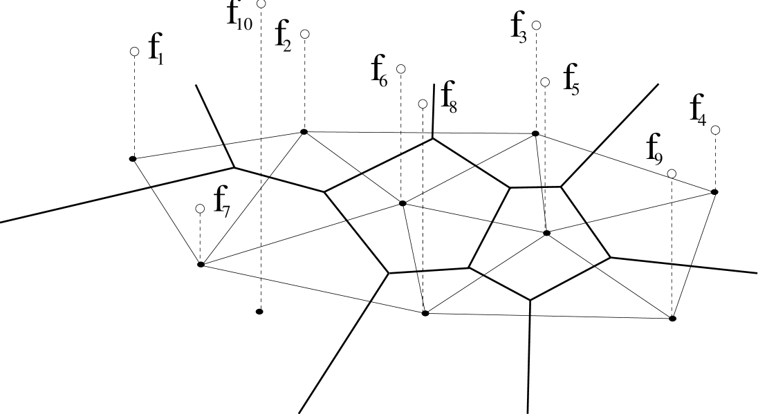
FIG. 2.: A Sectional Voronoï Partition (SVP) of the plane is defined by intersecting a three-dimensional Voronoï Partition with that plane. Sources $P_{i}$ of this SVP (black dots) are the projections of the three-dimensional sources $f_{i}$ (white dots) onto the plane. Interfaces $\Gamma_{ij}$ between cells are rectilinear, normal to $\overline{P_{i}P_{j}}$ and meet at triple vertices $v_{ijk}$, but are not equidistant from the sources. Sources with a too large value of $z_{i}$ (for example $P_{1}0$ in this figure) do not have an associated cell.

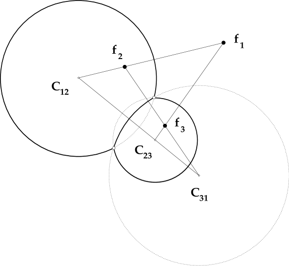
FIG. 3.: A Multiplicative Voronoï Partition with respect to three sources in two dimensions. The source with the largest intensity $a_{i}$ (source $f_{1}$ in this figure) has an unbounded cell. The other two sources are within their associated cells. Angles formed by the interfaces at the vertices are depend on the positions of the sources and the values of the intensities. For certain values of $\{a_{i}\}$ the interfaces may not intersect. In this case the partition would be composed of two disjoint circles containig one of the sources with smaller intensities each. The MVP with respect to three sources in three-dimensional space is a cluster of two spherical bubbles (Fig. 4, dashed lines).

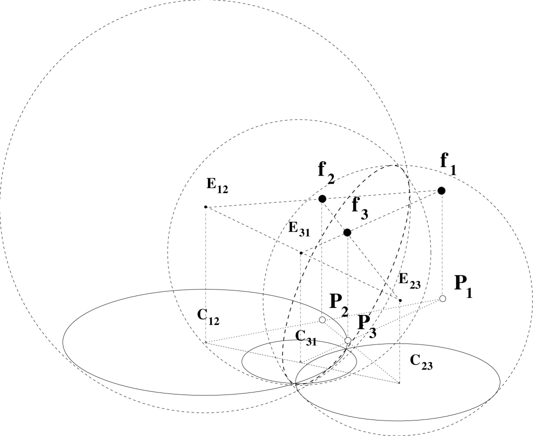
FIG. 4.: A Sectional Multiplicative Voronoï Partition (SMVP) is defined as a plane section (black circles) of a three-dimensional Multiplicative Voronoï Partition (dashed lines). Here an example for three sources. Sources $P_{i}$ of the SMVP (on the $\Pi_{z}$ plane, white dots), are the projections of sources $f_{i}$ of the MVP in three dimensions (black dots). The centers $E_{ij}$ of the 3d MVP are aligned, which implies the alignement of the centers $C_{ij}$ of the SMVP. Segments $\overline{f_{i}f_{j}}$ are normal to spheres $\tilde{\Gamma}_{i}j$, therefore $\overline{P_{i}P_{j}}$ are normal to circles $\Gamma_{ij}$ on the plane.

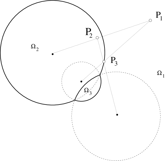
FIG. 5.: An upper view of the SMVP with respect to three sources defined in Fig. 4. Notice that sources $P_{i}$ are not all contained in their cell $\Omega_{i}$, as happens in the case of the MVP (Fig. 4).

FIG. 6.: A SMVP of the plane with six sources. The projections $P_{i}$ of the sources are indicated as small dots in the figure. For each one of the vertices in this partition, the three interfaces can be continued and they will meet each other again at a conjugatevertex.

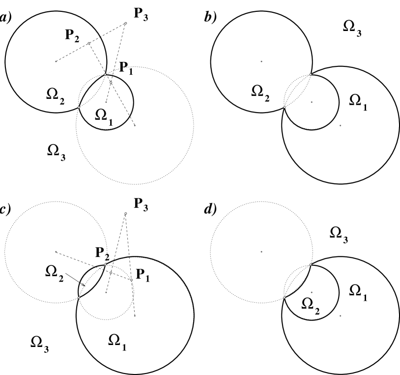
FIG. 7.: All these four circular vertices admit a reciprocal figure. Two of the vertices, a) and c), are convex and therefore a reciprocal figure satisfying orientation is possible. The other two are not convex so no reciprocal figure can satisfy orientation on them.

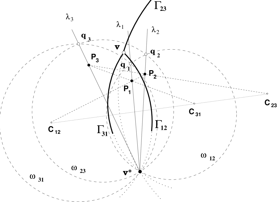
FIG. 8.: A vertex $v$ with its reciprocal figure $P_{1}P_{2}P_{3}$, showing circles $\omega_{ij}$. These circles are normal to the interfaces $\Gamma_{ij}$, and intersect each other at points $q_{i}$ on $\lambda_{i}$.

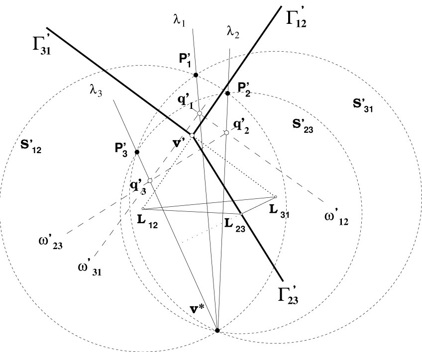
FIG. 9.: Same as Fig. 8, after an inversion around $v^{*}$. All circles originally through $v^{*}$ are now straight lines. This is the case of interfaces $\Gamma_{ij}$ and therefore we call this the “straight” representation of the vertex.

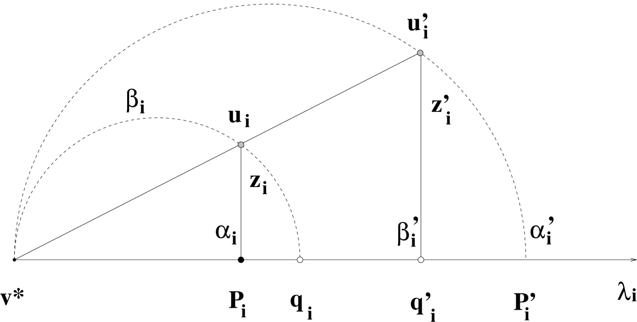
FIG. 10.: Shown is a plane normal to $\Pi_{z}$ and containing $\lambda_{i}$. This figure shows how the height $z_{i}$ of source $f_{i}=u_{i}$ in the original system is determined, given the positions of $P_{i}$ and $q_{i}$. Primed variables correspond to positions after the inversion, that is, in the “straight” system. Sources $f_{i}^{\prime}=u_{i}^{\prime}$ are above $q_{i}^{\prime}$, and therefore the back-transformed sources $f_{i}$ are above $P_{i}$.

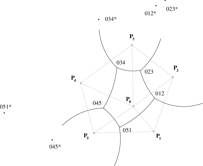
FIG. 11.: The points $P_{i}$ of the reciprocal figure (empty circles) are the projections, on the $xy$ plane, of the sources $f_{i}$ in three-dimensional space. The lines $\overline{P_{i}P_{j}}$ must thus be normal to interfaces $\Gamma_{ij}$. Black dots indicate the location of the conjugate vertices $v^{*}_{ijk}$ for each vertex $v_{ijk}$ in the figure.

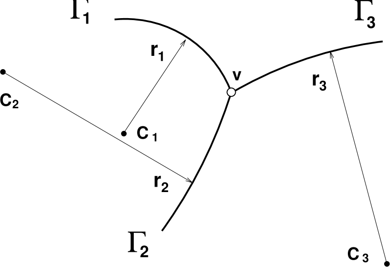
FIG. 12.: A generic vertex $v$, at which three interfaces $\Gamma_{1}$, $\Gamma_{2}$ and $\Gamma_{3}$ meet. We regard pressure drops to be positive if the pressure decreases when the interface is crossed in the counterclockwise sense of rotation around $v$. Therefore in the case shown in this figure, $r_{2}$ and $r_{3}$ are positive, while $r_{1}$ is negative.

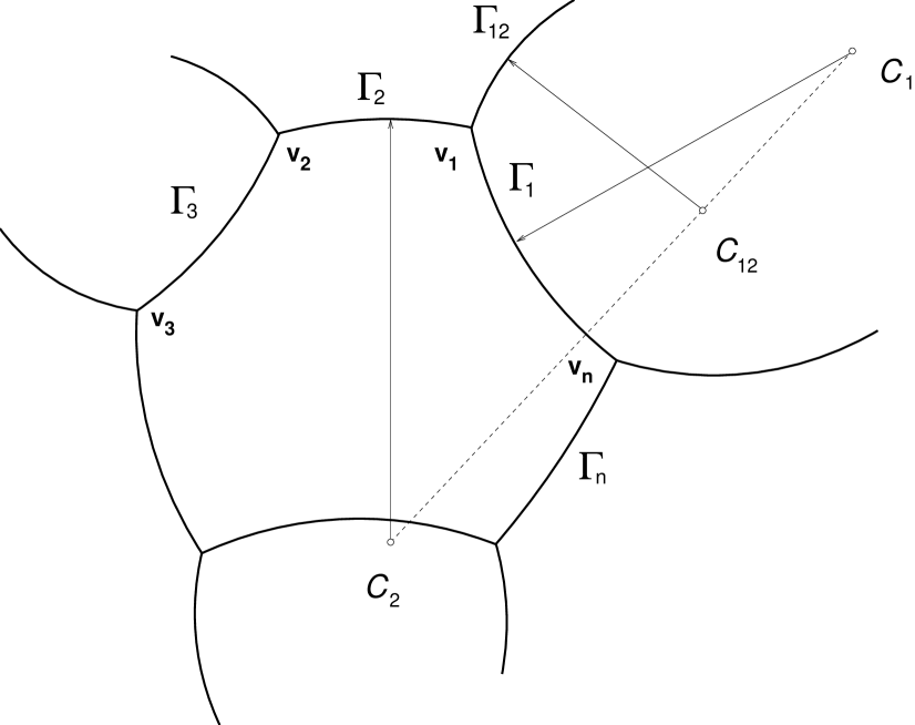
FIG. 13.: A bubble surrounded by $n$ neighbors $\alpha=1,\ldots,n$, showing the naming convention for the interfaces. Notice that film curvatures are of opposite signs when considered from each of the two vertices at their ends. Thus for example $\xi_{2}$ appears with $+$ sign in the equilibrium condition of vertex $v_{2}$, but with $-$ sign in that of $v_{1}$ (See equation 21).

FIG. 14.: The same closed bubble of Fig. 13, showing the film centers $C_{ij}$ (empty dots) aligned in triplets, and the sites $0,1,\ldots,6$ (black dots) of the reciprocal figure.

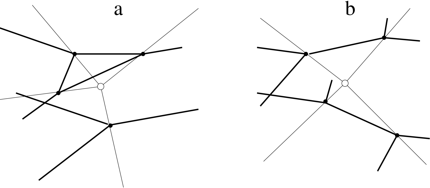
FIG. 15.: A three-dimensional Multiplicative Voronoï Partition gives rise to vertices which simultaneously belong to four neighboring bubbles in a generic situation. Six spherical interfaces converge at these vertices. When one such vertex (white dot) crosses the projection plane $\Pi_{z}$, depending on its orientation this can result either in a) a $T2$ process (disappearance of a triangular bubble) or b) a $T1$ process (neighbor switching) for the two-dimensional foam.

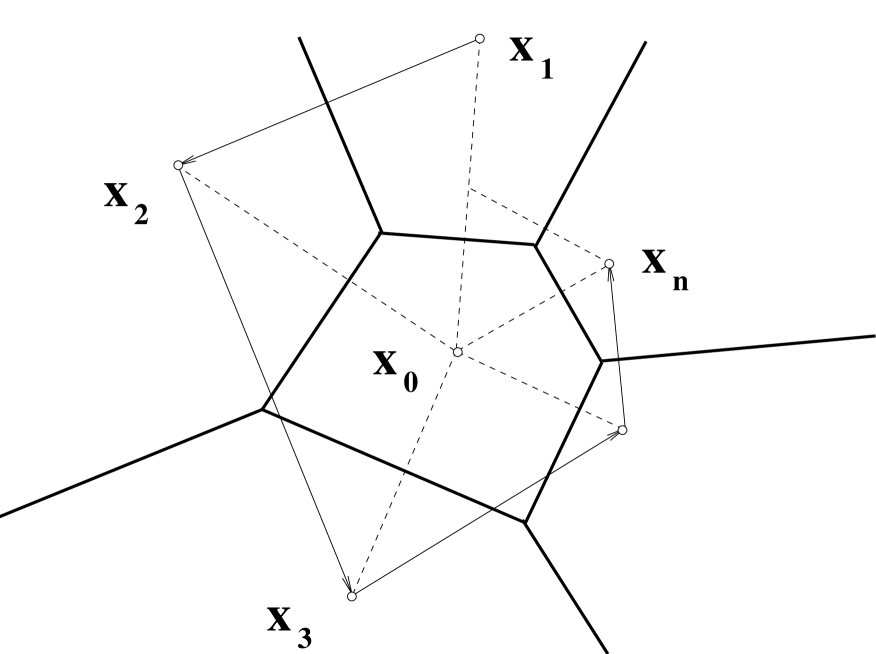
FIG. 16.: An arbitrary rectilinear partition will not in general admit a reciprocal figure. The one in this example does not admit a reciprocal figure, and therefore cannot be a Sectional Voronoï Partition.

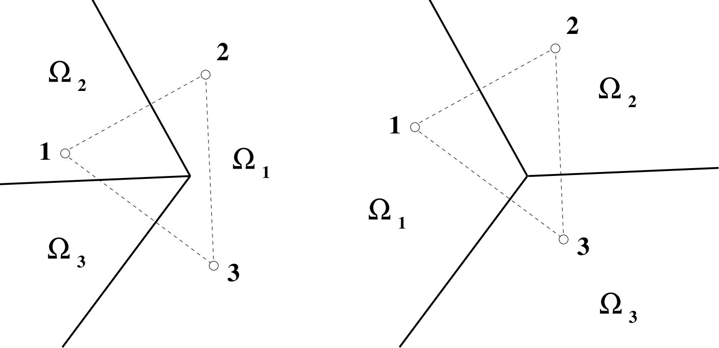
FIG. 17.: Both these partitions with three cells admit a reciprocal figure. The one on the left does not satisfy orientation and therefore cannot be part of a Sectional Voronoï Partition. The one on the right satisfies orientation, and therefore it is a SVP. It is then possible to find sources $f_{1}$, $f_{2}$ and $f_{3}$ in three-dimensional space, such that this partition is obtained as the cut $z=0$ of a three-dimensional Voronoï Partition with respect to $\{f_{i}\}$. Sources $f_{i}$ will be located at heights $z_{i}$ above points $\{1,2,3\}$ in this figure.

FIG. 18.: A convex rectilinear partition (thick lines) with cells $\{A,B,\ldots,I\}$ and its associated reciprocal figure (thin lines) with sites $\{a,b,\ldots,i\}$ (black dots). This reciprocal figure (or any other figure obtained from dilatation and translation of this one) satisfies orientation, and therefore the partition is a Sectional Voronoï Partition. Sources of this SVP are located above points $P_{i}$.

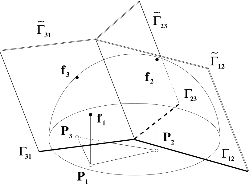
FIG. 19.: Given an oriented reciprocal figure $\{P_{1},P_{2},P3\}$ (white dots) for a rectilinear partition (interfaces $\Gamma_{ij}$), the sources $f_{i}$ in three dimensional space can be located above the points $P_{i}$. These sources must be equidistant from the vertex, therefore they are at the intersections (black dots) of a spherical surface centered at the vertex $v_{123}$ with the normals through $P_{i}$.

REFERENCES

- [1] N. Rivier, On the structure of random tissues or froths, and their evolution., Philosophical Magazine B 47 (1983), L45-L49.
- [2] D. Weaire and N. Rivier, Soap, Cells and Statistics—Random Patterns in Two Dimensions, Contemp. Phys. 25 (1984), 59-99.
- [3] J. Glazier and D. Weaire, The kinetics of cellular patterns, J.Phys.:Condens. Matter 4, (1992), 1867-1894.
- [4] J. Stavans, The evolution of cellular patterns, Rep. Prog. Phys. 56 (1993), 733-789.
- [5] C. S. Smith, The Shape of Things, Sci. Am. 190 (1954), 58.
- [6] C. S. Smith, Grain shapes and other metallurgical applications of topology, in: Metal Interfaces, Am. Soc. Metals, Cleveland, 1952.
-
[7]
D. Weaire and J. Kermode, Computer simulation of a two-dimensional
soap froth I. Method and motivation, Philosophical Magazine B 48
(1983), 245-259.
J. Kermode and D. Weaire, 2D-FROTH: a program for the investigation of 2-dimensional froths, Comput. Phys. Commun. 60 (1990), 75-109.
T. Herdtle and H. Aref, Numerical experiments on a two-dimensional foam, J. Fluid Mech. 241 (1992), 233-260. -
[8]
H. Flyvbjerg and C. Jeppesen, A Solvable Model
for Coarsening Soap Froths and Other Domain Boundary Networks in Two
Dimensions, Physica Scripta T38, (1991), 49-54.
H. Flyvbjerg, Dynamics of Soap Froth, Physica A 194,(1993), 298.
H. Flyvbjerg, Model for coarsening froths and foams, Phys. Rev. E 47, (1993), 4037. -
[9]
K. Kawazaki, T. Nagai and K. Nakashima, Phil. Mag. B
60, (1989), 399.
K. Kawasaki, Physica A 163, (1990), 59. - [10] Spatial Tessellations. Concepts and Applications of Voronoi Diagrams., A. Okabe, B. Boots and K. Sugihara, Wiley 1992.
- [11] H. Honda, Description of Cellular Patterns by Dirichlet Domains: The Two-Dimensional Case, J. Theor. Biol. 72, (1978), 523.
- [12] V. Icke and R. van de Weygaert, Fragmenting the Universe. I. Statistics of two-dimensional Voronoi foams, Astron. Astrophys. 184, (1987), 16-32.
- [13] Hiroshi Imai, Masao Iri and Kazuo Murota, Voronoï diagram in the Laguerre geometry and its applications., SIAM J. Comput. 14, (1985), 93.
- [14] B. N. Boots, Weighting Thiessen Polygons, Economic Geography (1979), 248-259.
-
[15]
Soap Bubbles, C. Vernon Boys, NY: Dover 1959,
pp. 120-127.
Reprinted in: The World of Mathematics , Tempus Books of Microsoft Press 1988 vol. II, pp. 883-886. - [16] On Growth and Form, D’arcy Wentworth Thompson, Cambridge University Press 1961, page 96.
- [17] Maxwell, J. C. On Reciprocal Figures and Diagrams of Forces, Phil. Mag. Series 4 (1864),250-261.
- [18] Maxwell, J. C. On Reciprocal Figures, Frames, and Diagrams of Forces, Trans. Royal Soc. Edinburgh 26 (1869-72),1-40.
- [19] Peter F. Ash and Ethan D. Bolker, Generalized Dirichlet Tessellations, Geometriae Dedicata 20 (1986),209-243.
- [20] Henry Crapo, Structural Rigidity, Structural Topology 1 (1979), 26-45.
- [21] Walter Whiteley, Realizability of Polyhedra, Structural Topology, 1 (1979), 46-58.
- [22] H. Telley, Modelisation et Simulation Bidimensionelle de la Croissance des Polycrystaux, Unpublished, Thesis Report N. 780. Ecole Polytechnique Federale de Lausanne, (1989).
- [23] This is called “phantom vertex” in [19].
- [24] Introduction to Geometry, H. S. M. Coxeter, Second Edition, Wiley and Sons 1989.
- [25] A configuration is formed by points and lines, such that each line is adjacent to points, and each point is adjacent to lines. See for example, Geometry and the Imagination, D. Hilbert and S. Cohn-Vossen, Chelsea Publishing Co., New York 1952, chapter III.
- [26] C. Moukarzel,Voronoi Foams, Physica A 199 (1993),19-30.
- [27] K. Lauritsen, C. Moukarzel and H. J. Herrmann, Statistical Physics and Mechanics of Random Lattices, J. Physique I (France) 3 (1993),1941.
- [28] C. Moukarzel, to be published.
- [29] Within our generalized notion of distance, that is, including the multiplicative constants.
- [30] Although it is statically unstable, a foam all of whose films are under compression would also be geometrically possible.