Scaling and Crossover Functions for the Conductance in the Directed Network Model of Edge States

Abstract

We consider the directed network (DN) of edge states on the surface of a cylinder of length $L$ and circumference $C$. By mapping it to a ferromagnetic superspin chain, and using a scaling analysis, we show its equivalence to a one-dimensional supersymmetric nonlinear sigma model in the scaling limit, for any value of the ratio $L/C$, except for short systems where $L$ is less than of order $C^{1/2}$. For the sigma model, the universal crossover functions for the conductance and its variance have been determined previously. We also show that the DN model can be mapped directly onto the random matrix (Fokker-Planck) approach to disordered quasi-one-dimensional wires, which implies that the entire distribution of the conductance is the same as in the latter system, for any value of $L/C$ in the same scaling limit. The results of Chalker and Dohmen are explained quantitatively.

I Introduction

Disordered conductors have been at the focus of experimental and theoretical research for quite some time. Even properties of a single electron in random potential are quite nontrivial. One of the challenging problems still open in this area is the description of the transition between the plateaus in the integer quantum Hall (QH) effect. Chalker and Coddington [1] introduced a network model to deal with this problem, and studied it numerically. Later several authors mapped this model to an antiferromagnetic spin chain, using replicas or supersymmetry to average over the disorder [2, 3, 4, 5]. The analysis of this spin chain is still complicated, and this model is not solved at present.

Recently Chalker and Dohmen [6] introduced a three-dimensional (3D) version of the network model to study the possibility of QH effect in 3D conductors. This 3D network models a conductor composed of stacked coupled layers perpendicular to a strong magnetic field. Each layer may separately exhibit the QH transition and is represented by the usual 2D network. In this system there exists a phase in which each individual layer is in the middle of a QH plateau, and all the electronic states in the bulk are localized. The only current-carrying states are the edge states on the surface of the conductor. These chiral surface states were studied in [5, 6, 7, 8, 9, 10]. In the framework of the network model, these surface states form a 2D directed network (DN), equivalent to one studied before [11]. A distinguishing feature of the model studied by Chalker and Dohmen is the periodic boundary condition on the edge of each layer, making the system the surface of a cylinder.

In this paper, we study (following Chalker and Dohmen) the conductance properties along the axis of the cylinder in the DN model. The paper is organized as follows. We set up a general formalism for the description of the DN model using supersymmetry and the approach of Ref. [2] in section II. Then we go to a continuum limit, and map the DN model to a spin chain in section III (this was also done in Refs. [5, 7, 8]). Unlike the case of the QH transition, this spin chain is ferromagnetic. This allows us to analyze its properties using ideas of a recent paper on continuum quantum ferromagnets [12]. Scaling arguments, similar to those of Ref. [12], show that all the moments of the conductance and other observables behave universally in the scaling limit (i.e. are given by universal scaling functions of dimensionless combinations of the bare couplings of the continuum model).

In particular, we show that when the ferromagnetic chain under consideration is in the classical regime (called “renormalized” classical in Ref. [12], but we drop the modifier because, due to the no-scale-factor universality [12], no coupling constants are renormalized), it can be further reduced to a 1D classical non-linear sigma model, studied before by Mirlin et al. in the context of localization in quasi-1D wires [13]. Based on this reduction we show that in this classical scaling regime all the moments of the conductance $g$ are the same for both models. Thus, borrowing results of Ref. [13], we can fully determine the crossover functions for the mean and variance of the conductance of the DN model for any ratio of the length and circumference of the cylinder in the scaling regime. This classical scaling regime does not include the regime of very small $L<{\cal O}(C^{1/2})$ that was termed 0D in Ref. [8].

A recent paper [14] shows how one can in principle obtain the full probability distribution of the transmission eigenvalues from the non-linear sigma model, and proves that this distribution is identical to the one obtained from the Dorokhov-Mello-Pereyra-Kumar (DMPK) equation [15, 16] of the Fokker-Planck (FP) approach which describes the universal behavior of localization in quasi-1D wires. In view of this equivalence, the probability distribution of the conductance of the DN model in the classical scaling regime is the same as that of the quasi-1D model. For the quasi-1D model, a lot is known exactly about this distribution [17], and thus a nearly complete description of the conductance properties of the DN model is available. In section IV we give a direct argument that shows how the DN model is related to a quasi-1D model, and thus to the DMPK equation. We compare our results with those of Chalker and Dohmen [6]. We conclude in section V.

II The Directed Network Model: General Setup and the Symmetry

The DN is shown in Fig. 1 and consists of links and nodes. The links carry complex fluxes, and the nodes represent (unitary) scattering matrices ${\cal S}$ connecting incoming $(i,i^{\prime})$ and outgoing $(o,o^{\prime})$ fluxes:

$$\left(\begin{array}[]{c}o\\ o^{\prime}\end{array}\right)={\cal S}\left(\begin{array}[]{c}i\\ i^{\prime}\end{array}\right)=\left(\begin{array}[]{cc}\alpha&\beta\\ \gamma&\delta\end{array}\right)\left(\begin{array}[]{c}i\\ i^{\prime}\end{array}\right).$$ (1)

The scattering amplitudes $\alpha,\ldots,\delta$ correspond to elementary scattering events shown on the right in Fig. 1. For the time being they are assumed to be arbitrary complex numbers different for different nodes, which allows us to formulate our model for disordered samples with any realization of disorder. A particular distribution for the scattering amplitudes will be specified later. The vertical direction in Fig. 1 is along the circumference of the cylinder. Later it will play the role of imaginary time for the spin chain, so we call the vertical coordinate $\tau$. In the $\tau$-direction the network has the size $C=N_{\tau}a_{\tau}$ where $N_{\tau}$ is the number of “channels” through the system and $a_{\tau}$ is a microscopic scale of the order of the mean free path of electrons. We impose periodic boundary conditions in this direction. In the $x$-direction the network has finite length $L=Na_{x}$, where $N$ is the number of layers (or “sites”), and $a_{x}$ is the distance between them. In this direction the system is connected to ideal leads. In Fig. 1 the edge states are numbered from 1 to $N=5$, and $N_{\tau}=3$.

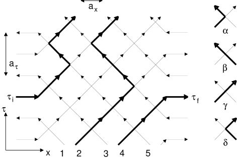
FIG. 1.: The directed network (DN) model. The particles move on the links in the directions shown by the arrows. The bold line represents a typical path. The scattering amplitudes on such a path are as shown on the right.

Different correlation functions may be defined for this model and each of them may be represented in the first or second quantized way. As an illustrative and important example, we derive expressions for the conductance. The dimensionless conductance is given by the Landauer formula $g=\mbox{tr \boldmath$t^{\dagger}t$}=\sum_{i,f}|t_{if}|^{2}$, where $t$ is the total transmission matrix (with matrix elements $t_{if}$) between left and right boundaries of the system. In the first quantized language, $t_{if}$ is given by the sum over “retarded” paths connecting an incoming link at $\tau_{i}$ on the left boundary and an outgoing link at $\tau_{f}$ on the right boundary. Each path follows links only in the direction of the arrows and its contribution is the product of the scattering amplitudes along the path. One such path is shown on Fig. 1 with bold lines. Similarly, $t_{if}^{*}$ is given by the sum over “advanced” paths where each node contributes the complex conjugate scattering amplitude.

In the second quantized language, the sum over paths may be written as a trace of an “evolution” operator in a Fock space of bosons and fermions. To represent $t_{if}$ ($t_{if}^{*}$) we introduce a retarded (advanced) boson $a_{i}$ ($b_{i}$) and fermion $f_{i}$ ($g_{i}$) on each link $i$. The numbers of bits of paths on each link play the role of occupation numbers of these bosons and fermions, and the collection of these numbers on horizontal section at a given $\tau$-coordinate specifies a state in the Fock space. Then the evolution operator $V_{12}$ for a single node between the sites 1 and 2, which evolves quantum states on these sites by one step in the $\tau$-direction, is given by the sum of the contributions of all possible scattering events, described by ${\cal S}$. In a typical event involving only retarded bosons, $k$ bosons are transferred from site 1 to site 2 with amplitude $\gamma$, $l$ bosons are transferred from site 2 to site 1 with amplitude $\beta$, and the remaining bosons stay on their respective sites, each contributing factors $\alpha$ for site 1 and $\delta$ for site 2. This event gives the term $(\gamma^{k}\beta^{l}\!/{k!\,l!})(a^{\dagger}_{2})^{k}(a^{\dagger}_{1})^{l}\alpha^{n_{a1}}\delta^{n_{a2}}a_{2}^{l}a_{1}^{k}$ (where $n_{a1}=a^{\dagger}_{1}a_{1}$ etc.) in the evolution operator $V_{12}$. After some rearrangement, the sum of all such terms for all the bosons and fermions may be written as

$$V_{12} = :\exp\biggl{(}{\gamma\over\alpha}(a^{\dagger}_{2}a_{1}+f^{\dagger}_{2}f_{1})+{\beta\over\delta}(a^{\dagger}_{1}a_{2}+f^{\dagger}_{1}f_{2})$$ (4)

$$+{\gamma^{*}\over\alpha^{*}}(b^{\dagger}_{2}b_{1}+g^{\dagger}_{2}g_{1})+{\beta^{*}\over\delta^{*}}(b^{\dagger}_{1}b_{2}+g^{\dagger}_{1}g_{2})\biggr{)}:$$

$$\times\alpha^{n_{a1}+n_{f1}}(\alpha^{*})^{n_{b1}+n_{g1}}\delta^{n_{a2}+n_{f2}}(\delta^{*})^{n_{b2}+n_{g2}},$$

where colons stand for normal ordering.

The contribution of the boundary nodes connected to the leads is different. When representing $|t_{if}|^{2}$, every leftmost node at $\tau\neq\tau_{i}$ has only paths reflected off the left boundary (with the corresponding amplitude $\delta$ or $\delta^{*}$), because only such paths contribute to $|t_{if}|^{2}$. Then the only possible event at such a node is that all the particles stay on the site 1, each contributing factors $\delta$ for retarded and $\delta^{*}$ for advanced ones. The corresponding evolution operator is simply

$$V_{01}=\delta^{n_{a1}+n_{f1}}(\delta^{*})^{n_{b1}+n_{g1}}.$$ (5)

For the leftmost node at $\tau_{i}$ we also need to inject one retarded and one advanced path into the system. This is represented by the event where we create additional retarded and advanced particles on the site 1. For definiteness we choose them to be bosons. The corresponding evolution operator is $|\gamma|^{2}a^{\dagger}_{1}b^{\dagger}_{1}\delta^{n_{a1}+n_{f1}}(\delta^{*})^{n_{b1}+n_{g1}}=|\gamma|^{2}a^{\dagger}_{1}b^{\dagger}_{1}V_{01}$. Similarly, for the rightmost nodes at $\tau\neq\tau_{f}$ we have

$$V_{N,N+1}=\alpha^{n_{aN}+n_{fN}}(\alpha^{*})^{n_{bN}+n_{gN}},$$ (6)

and for the boundary node at $\tau_{f}$ the evolution operator is $|\gamma|^{2}V_{N,N+1}a_{N}b_{N}$.

The total evolution operator $U$ is composed of all the $V_{i,i+1}$’s in the following manner. Assume for definiteness that the number of sites $N$ is odd. Then in our system we have even rows of links at integer times $0,a_{\tau},2a_{\tau}$, etc., where fluxes enter the system from the left and exit it to the right, and odd rows of links at half-integer times $a_{\tau}/2,3a_{\tau}/2$, etc., where fluxes enter from the right and exit to the left. For even rows we form the product

$$V_{e}(\tau)=V_{01}(\tau)V_{23}(\tau)\ldots V_{N-1,N}(\tau),$$ (7)

and for odd ones

$$V_{o}(\tau)=V_{12}(\tau)V_{34}(\tau)\ldots V_{N,N+1}(\tau).$$ (8)

The operator $U$ is then given by the product

$$U=\prod_{n=0}^{N_{\tau}-1}V_{o}\Bigl{(}(n+1/2)a_{\tau}\Bigr{)}V_{e}\Bigl{(}na_{\tau}\Bigr{)},$$ (9)

which is ordered with the earliest times at the right. Note that the only $\tau$-dependence in the operators $V_{e}$, $V_{o}$ is through the ${\cal S}$-matrix elements, which implicitly depend on $i$ and $\tau$.

With the help of the operator $U$, the conductance is given by

$$g={\rm STr}\biggl{(}{\cal T}\!\sum_{\tau_{i},\tau_{f}}|\gamma_{i}|^{2}a^{\dagger}_{1}(\tau_{i})b^{\dagger}_{1}(\tau_{i})|\gamma_{f}|^{2}a_{N}(\tau_{f})b_{N}(\tau_{f})\,U\biggr{)}\!.$$ (10)

Here $\tau_{i}$ and $\tau_{f}$ label the times at which the creation and annihilation operators act on the states, $\gamma_{i}$ and $\gamma_{f}$ are the ${\cal S}$ matrix elements at the corresponding nodes, and ${\cal T}$ orders times, placing the earliest at the right. “STr” stands for the supertrace in the Fock space, which weights all the states with the factor of $(-1)^{N_{F}}$, where $N_{F}=\sum_{i=1}^{N}(n_{fi}+n_{gi})$ is the total number of fermions in a state, ${\rm STr}(\ldots)={\rm Tr}((-1)^{N_{F}}\ldots)$. That is, states with an odd number of fermions contribute to the sum with a negative sign. This, together with the periodicity in the $\tau$-direction, ensures the cancellation of bosonic and fermionic contributions from closed paths not connected to the leads. These closed paths were, as usual, absent from the original first quantized formulation of the problem.

In Eq. (10), $\tau_{i}$ and $\tau_{f}$ take only half-integer values $a_{\tau}/2$, $3a_{\tau}/2$, so on, because we create and destroy bosons only on half of the links belonging to the sites 1 and $N$. Using the commutation relations between the bosonic operators and $V$’s, we can rewrite the expression for $g$ in the form

$$g={\rm STr}\biggl{(}{\cal T}\sum_{\tau}\varepsilon_{\tau}a^{\dagger}_{1}(\tau)b^{\dagger}_{1}(\tau)\sum_{\tau^{\prime}}\varepsilon_{\tau^{\prime}}a_{N}(\tau^{\prime})b_{N}(\tau^{\prime})\,U\biggr{)}\!,$$ (11)

where now $\tau$ and $\tau^{\prime}$ take all possible values, but $\varepsilon_{\tau}=1$ ($-1$) for integer (half-integer) values of $\tau/a_{\tau}$.

This is a good place in which to discuss in more detail the choice of boundary conditions for our model. In the $x$-direction the presence of the ideal absorbing leads at the boundaries of the system means in the first quantized language that we do not include contributions from the paths leaving or entering the system unless we specifically calculate some correlators between the boundaries (like conductance $g$). In the second quantized language this translates to the following. We can imagine having two additional vertical sets of links in the leads (0th and $N+1$st sites) on which we have no bosons or fermions, so these sites always carry the vacuum state $|0\rangle$. With this constraint the boundary operators $V_{01}$ and $V_{N,N+1}$ are seen to be special forms of general $V_{i,i+1}$’s, Eq. (4), acting on the vacuum at the left or right. Later this constraint on the states at the boundaries will give, in the $\tau$-continuum formulation, the symmetry-breaking term in the Hamiltonian and in the action, and will fix the boundary conditions in the continuum field theory, see Eq. (23) below.

We now discuss the supersymmetry properties of our formulation. For each site $i$ we can form 16 bilinears in our bosonic and fermionic operators. They represent the 16 generators of the Lie superalgebra $u(1,1\,|\,2)$. We arrange these generators in a $4\times 4$ matrix, or “superspin” $J_{i}$:

$$J_{i}=\!\!\left(\!\!\begin{array}[]{cccc}a_{i}a^{\dagger}_{i}-1/2&a_{i}f^{\dagger}_{i}&a_{i}b_{i}&a_{i}g_{i}\\ f_{i}a^{\dagger}_{i}&f_{i}f^{\dagger}_{i}-1/2&f_{i}b_{i}&f_{i}g_{i}\\ -b^{\dagger}_{i}a^{\dagger}_{i}&-b^{\dagger}_{i}f^{\dagger}_{i}&-b^{\dagger}_{i}b_{i}-1/2&-b^{\dagger}_{i}g_{i}\\ g^{\dagger}_{i}a^{\dagger}_{i}&g^{\dagger}_{i}f^{\dagger}_{i}&g^{\dagger}_{i}b_{i}&g^{\dagger}_{i}g_{i}-1/2\end{array}\!\!\right)\!.$$ (12)

We adopted “advanced-retarded” arrangement of the generators rather than the “boson-fermion” one (see [4] for details). In this scheme the diagonal $2\times 2$ blocks of $J_{i}$ contain the generators of the subalgebra $u(1\,|\,1)\oplus u(1\,|\,1)$. Then one can show that the operator $V_{12}$ commutes with all 16 components of $J_{1}+J_{2}$ (and thus has $u(1,1\,|\,2)$ as the symmetry algebra),

$$(J_{1}+J_{2})\,V_{12}=V_{12}\,(J_{1}+J_{2}),$$ (13)

if and only if the scattering matrix ${\cal S}$ is unitary: ${\cal S}^{-1}={\cal S}^{\dagger}$ (the analogous result for the Chalker-Coddington model was found in Ref. [2]). Thus, the products of the $V_{i,i+1}$’s in $V_{e}$ and $V_{o}$ commute with the total superspin $\sum_{i=1}^{N}J_{i}$ for any realization of disorder, provided that all the scattering matrices are unitary, except for the boundary operators $V_{01}$ and $V_{N,N+1}$. These boundary operators commute only with generators from diagonal blocks of $J_{1}$ and $J_{N}$, correspondingly, and break the symmetry of the total evolution operator $U$ down to $u(1\,|\,1)\oplus u(1\,|\,1)$. Therefore, for any realization of the disorder, unitarity of the scattering matrices ensures the global $u(1,1\,|\,2)$ symmetry of our problem, which is broken only by the boundary constraint. The use of the supertrace, not the ordinary trace, is essential in maintaining the supersymmetry in the presence of the periodicity in the $\tau$-direction.

In terms of the superspins, Eq. (11) for the conductance may be rewritten as

$$g={\rm STr}\biggl{(}{\cal T}\sum_{\tau}\varepsilon_{\tau}J_{1}^{31}(\tau)\sum_{\tau^{\prime}}\varepsilon_{\tau^{\prime}}(-1)^{N}J_{N}^{13}(\tau^{\prime})\,U\biggr{)}\!.$$ (14)

Here $J_{1}^{31}=-b^{\dagger}_{1}a^{\dagger}_{1},J_{N}^{13}=a_{N}b_{N}$ are particular components of superspins $J_{1}$ and $J_{N}$ at the boundaries of the system. The alternating sums of the type

$${\cal I}_{i}=(-1)^{i}\sum_{\tau}\varepsilon_{\tau}J_{i}^{ab}(\tau)$$ (15)

represent the total current through the system in the $x$-direction. Using the supersymmetry of the operators $V$, Eq. (13), we can show that this current is conserved, i.e., correlators of ${\cal I}_{i}$’s do not depend on the position labels $i$, except at the boundaries. We see then that Eq. (14) is the usual Kubo-type formula, relating the conductance to a current-current correlator, $g=-{\rm STr}({\cal T}\,{\cal I}_{i}{\cal I}_{j}U)$, for $i\neq j$.

Similarly we can write down expressions for the moments of the conductance or other correlators. For moments higher than the second, we need to introduce some additional structure. Namely, we introduce $n$ replicas of our bosons and fermions and sum the bilinear operators in the exponentials in the expressions for $V_{i,i+1}$’s over replica indices. This is necessary, because to represent the $m$-th power of the conductance we need to create at the boundary $m$ different retarded and $m$ different advanced particles, and we need $n\geq m/2$. The corresponding model has global $u(n,n\,|\,2n)$ symmetry broken down to $u(n\,|\,n)\oplus u(n\,|\,n)$ by the boundary constraint. We should point out that in this case replicas are not introduced to average over the disorder, and their number $n$ is not taken to zero in the end. In this model, results for the $m$-th moment are independent of $n$, provided $m\leq 2n$, because any “excess” replicas cancel by supersymmetry. For simplicity we continue to assume $n=1$.

So far we did not have to specify the nature of the disorder. Now we assume a particular distribution of the scattering matrices, used before in [1, 6]. Namely, we take every scattering matrix to consist of a product of two diagonal unitary matrices with a real orthogonal matrix, with entries

$$-\beta=\gamma=t>0,\quad\alpha=\delta=(1-t^{2})^{1/2},$$ (16)

in between them, the latter matrix being the same for all nodes. The phases from the diagonal unitary matrices are associated with links rather than with nodes and are assumed to be uniformly distributed between 0 and $2\pi$, independently for each link [1, 6]. Thus averaging over disorder corresponds to integration over all the link phases.

It is easy to see that this averaging produces a local constraint on the states in the Fock space. Let each retarded bit on a given link at the $i$-th site at time $\tau$ contribute the factor $e^{i\varphi}$, and each advanced one the factor $e^{-i\varphi}$, to the amplitude associated with a given path. Then if we have $m$ retarded and $n$ advanced bits on the link, averaging over random phase $\varphi$ gives $\int_{0}^{2\pi}\exp\bigl{(}i(m-n)\varphi\bigr{)}d\varphi=\delta_{m,n}$, that is, we get zero unless the number of retarded and advanced bits is the same. Thus, we have a local constraint on the number of bits of paths on each link. In the second-quantized language this means that the averaging projects our evolution operator to the subspace specified by $n_{ai}+n_{fi}=n_{bi}+n_{gi}$ for each $i$ and each time $\tau$. This subspace forms a highest weight irreducible representation of the algebra $u(1,1\,|\,2)$, with the vacuum $|0\rangle$ for the site $i$ being the “highest weight” vector. This representation was first obtained for the Chalker-Coddington model [1] in [2] and was also discussed in [4].

III Mapping to a Spin Chain and Scaling Analysis

So far in our derivation we retained discreteness of the DN. Unlike in the other published derivations [5, 7, 8], we did not have to take the time-continuum limit from the start. However, we do so now in order to obtain a continuum field theory for our system and to study its universal scaling properties. In the $\tau$-continuum limit we assume $t\ll 1$ and expand the $V_{i,i+1}$’s, projected to the constrained subspace, to second order in $t$. The result of the expansion is $V_{i,i+1}=1-t^{2}{\rm str}J_{i}J_{i+1}+{\cal O}(t^{4})$, where $J_{i}$ are superspins in the highest weight representation mentioned above. Here “str” stands for the matrix supertrace in the space labeled by the upper indices of $J_{i}^{ab}$. In other words, for any $4\times 4$ supermatrix $A$, str$A\equiv{\rm tr}\,\eta A$ where “tr” is the usual matrix trace and $\eta$ is a diagonal matrix with entries $(1,-1,1,-1)$. Now we combine all the $V$’s and reexponentiate. We also replace sums over $\tau$ by integrals. The result is the evolution operator in imaginary time $\tau$ of a 1D quantum ferromagnetic spin chain with Hamiltonian

$$H[J]={t^{2}\over a_{\tau}}\biggl{(}\sum_{i=1}^{N-1}{\rm str}J_{i}J_{i+1}+{1\over 2}{\rm str}\Lambda(J_{1}+J_{N})\biggr{)}.$$ (17)

Here $\Lambda$ is the diagonal matrix ${\rm diag}(1,1,-1,-1)$. The last term in $H$ comes from the boundary nodes. It may be interpreted as saying that there are, at the boundaries, two additional spins $J_{0}$ and $J_{N+1}$ fixed to a particular “direction” $J_{0}=J_{N+1}=\Lambda/2$ by an infinitely strong magnetic field coupling via a Zeeman term in the superspin space. This is another manifestation of the boundary constraint mentioned above.

Using the algebra of the generators $J^{ab}$ in the same $\tau$-continuum limit, the expression (15) for the total current becomes

$${\cal I}_{i}={t^{2}\over a_{\tau}}\int_{0}^{C}\!\!d\tau[J_{i},J_{i-1}]=-{t^{2}\over a_{\tau}}\int_{0}^{C}\!\!d\tau[J_{i},J_{i+1}].$$ (18)

For the particular components of the current at the boundaries these expressions reduce to ${\cal I}_{1}^{31}=(t^{2}/2a_{\tau})\int\!d\tau[J_{1},\Lambda]^{31}=(t^{2}/a_{\tau})\int\!d\tau J_{1}^{31}$ and, similarly, ${\cal I}_{N}^{13}=(t^{2}/a_{\tau})\int\!d\tau J_{N}^{13}$.

Next, we introduce supercoherent states and represent quantities of interest as path integrals over some supermanifold, see [8, 18] for details. The resulting theory has the action

$$S=S_{B}+\int_{0}^{C}\!\!d\tau H[Q(\tau)],$$ (19)

where $S_{B}$ is the Berry phase term (specified below), $Q_{i}(\tau)$ is a supermatrix taking values in the coset space $U(1,1\,|\,2)/U(1\,|\,1)\times U(1\,|\,1)$ (where $U(1,1\,|\,2)$ is the supergroup of which the Lie superalgebra is $u(1,1\,|\,2)$, etc.), and $H[Q(\tau)]$ is obtained from $H[J]$ by replacing every $J_{i}$ with $Q_{i}(\tau)/2$ (we make the same replacement in the expressions for the total current). In the path integral, all the components of $Q$ obey periodic boundary conditions. The difference, in the case of the fermionic components, from the usual path integrals for fermions, which obey antiperiodic boundary conditions [19], is a direct consequence of the factor $(-1)^{N_{F}}$ in the definition of STr.

The scaling properties of quantum ferromagnets were discussed in [12]. Following that paper, we take the spatial continuum limit of the action $S$ and the current ${\cal I}_{i}$. The resulting continuum ferromagnet has the action

$$S_{\rm cont} = -\int_{0}^{L}\!\!dx\!\!\int_{0}^{C}\!\!d\tau\biggl{(}\!{M_{0}\over 2}\!\!\int_{0}^{1}\!du\,{\rm str}\,Q(u){\partial Q(u)\over\partial u}{\partial Q(u)\over\partial\tau}$$ (21)

$$+{\rho_{s}\over 2}{\rm str}(\nabla Q)^{2}\biggr{)}\!,$$

and the current becomes

$${\cal I}(x)=-2\rho_{s}\int_{0}^{C}\!\!d\tau Q\nabla Q.$$ (22)

Here $M_{0}=1/2a_{x}$ and $\rho_{s}=t^{2}a_{x}/4a_{\tau}$ are the magnetization per unit length, and the spin stiffness in the ferromagnetic ground state respectively. Also, in the Berry phase term, the first term in $S_{\rm cont}$, $Q(u)\equiv Q(x,\tau,u)$ is some smooth homotopy between $Q(x,\tau,0)=\Lambda$ and $Q(x,\tau,1)=Q(x,\tau)$ (for details see [18]). The circumference of the cylinder $C$ plays the role of the inverse temperature. The last term in $H[Q(\tau)]$, or the interpretation $J_{0}=J_{N+1}=\Lambda/2$, forces the field $Q(x,\tau)$ to take the boundary values

$$Q(0,\tau)=Q(L,\tau)=\Lambda.$$ (23)

A boundary condition of this form to represent ideal absorbing leads is usual in the non-linear sigma model formulation of the theory of localization (to which, we note, the model (21) is not equivalent). Given that the effective supersymmetric spin system is ferromagnetic, and that fluctuations in the length of the spins can be neglected, the form of the action $S_{\rm cont}$ is dictated by the supersymmetry, which holds universally for any short range form of disorder.

The action (21) clearly shows an anisotropic scaling which reflects the difference between the $x$- and $\tau$-directions in the DN. In the original discrete version of the DN model, if we consider the local behavior without the periodic boundary condition, the mean conductivity behaves diffusively in the $x$-direction, with $\tau$ playing the role of time, with the diffusion constant

$$D={t^{2}\over 1-t^{2}}{a_{x}^{2}\over a_{\tau}},$$ (24)

as shown in Refs. [6, 11]. (However, even without the periodic boundary condition, less trivial behavior is found for higher moments [11].) In the spin chain language this anisotropy is manifest in the usual quadratic dispersion relation of the spin waves. The action (21), linearized near the ferromagnetic ground state, describes (on analytic continuation to real time) spin waves with the dispersion $\omega=2\rho_{s}k^{2}/M_{0}$. The difference between the ratio $2\rho_{s}/M_{0}=t^{2}a_{x}^{2}/a_{\tau}$ and the diffusion constant $D$ is due to the particular order of time- and space-continuum limits taken to obtain the action (21). The more general long wavelength behavior ($k_{x}a_{x}\ll 1$, $k_{\tau}a_{\tau}\ll 1$), consistent with Eq. (24), should be described by the same action $S_{\rm cont}$ but with the more accurate expression for the spin stiffness,

$$\rho_{s}={t^{2}\over 1-t^{2}}{a_{x}\over 4a_{\tau}}.$$ (25)

In general, the continuum description requires that $C\gg a_{\tau}$, $L\gg a_{x}$.

Although $S_{\rm cont}$ is a highly non-trivial interacting quantum field theory, it is nevertheless possible to make some simple exact statements about it. First, its “ground state” (which dominates the functional integral in the limit of zero “temperature”, $C=\infty$) is fully polarized and fluctuationless, so $\langle Q\rangle_{C=\infty}=\Lambda$. As a result, the parameter $M_{0}$, which measures the Berry phase due to adiabatic changes in the ground state polarization, cannot have any non-trivial zero temperature renormalization [12]. Second, not only the ground state, but some low-lying excited states are also known exactly: the linearized single spin-wave states are in fact exact eigenstates of the full Hamiltonian, and their dispersion $\omega=2\rho_{s}k^{2}/M_{0}$ has no corrections from the non-linearities. This implies that $\rho_{s}$ also has no non-trivial zero-temperature renormalization [12]. We also mention, as an aside, that the mapping from the DN model to $S_{\rm cont}$ can be generalized to higher spatial dimensions $d$. As a result, the critical dimension $d=2$ (for the properties at large $C$) pointed out in Ref. [12] is related to the same fact obtained in Ref. [11].

The absence of any non-trivial renormalizations of $M_{0}$ and $\rho_{s}$, the absence of any additional relevant operators in $1+1$ dimensions, and the related absence of ultraviolet divergences in physical quantities in the $1+1$-dimensional quantum field theory, are responsible for the phenomenon of “no-scale-factor universality” [12, 20]. Among its implications is that scaling analysis of $S_{\rm cont}$ reduces to the naive analysis of engineering dimensions. The field $Q(x,\tau)$, being subject to the constraint $Q^{2}(x,\tau)=1$, is dimensionless. Then simple power counting gives the engineering dimensions of the couplings: ${\rm dim}\,M_{0}=({\rm length})^{-1}$, ${\rm dim}\,\rho_{s}={\rm length/time}$. The no-scale-factor universality also implies that all the observables are functions of dimensionless combinations of the bare couplings $M_{0}$ and $\rho_{s}$ and the large scales, which, for the conductance, are just $L$ and $C$. For example, the mean conductance is given by a function

$$\langle g\rangle=\Phi_{g}\left(\frac{L}{(C\rho_{s}/M_{0})^{1/2}},\frac{L}{C\rho_{s}}\right).$$ (26)

Clearly, we could have chosen other combinations of the two arguments of the $\Phi_{g}$, and the physics behind our particular choices will become clear as we proceed. The continuum theory $S_{cont}$ applies to any particular lattice quantum ferromagnet provided the lengths $L,C$ are sufficiently large. Specifically [12], we require $M_{0}L\gg 1$ and $\rho_{s}M_{0}C\gg 1$ (or $L\gg a_{x}$ and $C\gg a_{\tau}(1-t^{2})/t^{2}$, as well as $C\gg a_{\tau}$). Comparing with the function $\Phi_{g}(\ell_{1},\ell_{2})$, we see that the condition on $C$ implies that $\ell_{1}\gg\ell_{2}$, and $\Phi_{g}$ becomes universal in this regime, with no non-universal factors in either the scale of $\Phi_{g}$ or its arguments. Notice that the arguments $\ell_{1}$, $\ell_{2}$ can take all positive value $0<\ell_{1},\ell_{2}\leq\infty$ while satisfying $\ell_{1}\gg\ell_{2}$. We also emphasize that the condition for universality may be satisfied for any ratio $L/C$, i.e. for short as well as long cylinders.

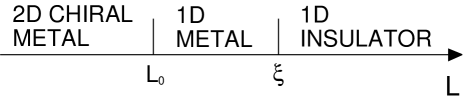
FIG. 2.: Sketch of the crossovers as a function of the length $L$. The first crossover [8] is at the scale $L\sim L_{0}=(C\rho_{s}/M_{0})^{1/2}$ where the low-lying energy level splittings of the quantum ferromagnet $\sim\rho_{s}/M_{0}L^{2}$ are of order the “temperature” $1/C$. The second crossover is near the localization length $\xi=8C\rho_{s}$. The conditions for the validity of the continuum theory require $\xi\gg L_{0}$, and so the two crossover scales are well separated. The quantum ferromagnet behaves classically for all $L\gg L_{0}$ (but with no restriction on $L/C\rho_{s}$) and is then described by the one-dimensional supersymmetric non-linear sigma model $S_{1}$ (Eq. (28)), which is therefore valid across the crossover at $L\sim C\rho_{s}$. The Fokker-Planck approach of Section IV has the same regime of validity ($L\gg L_{0}$, $L/C\rho_{s}$ arbitrary). The 2D chiral metal regime was labelled 0D in Ref. [8], but we prefer the present terminology for reasons discussed below Eq. (34).

We first present our results for the case $L\gg L_{0}\equiv(C\rho_{s}/M_{0})^{1/2}$. The length $L_{0}$ was identified in Ref. [8], and we will discuss the regime $L\leq L_{0}$ later (see Fig 2). For $L\gg L_{0}$, we have from (26)

$$\langle g\rangle=\Phi_{g1}\left({L\over C\rho_{s}}\right),$$ (27)

where $\Phi_{g1}(\ell)\equiv\Phi_{g}(\infty,\ell)$. Notice that the ratio $L/C$ is still allowed to be arbitrary. The form (27) implies that any localization length $\xi$ must obey $\xi\propto C\rho_{s}$, which was the basic result of Chalker and Dohmen [6], which we have now explained. One might have been tempted to use the incorrect naive argument, that distances in the $x$-direction (such as $\xi$) should scale as the square root of distances in the $\tau$-direction (such as $C$). However, under such scaling, $\rho_{s}$ is not scale invariant, while $C\rho_{s}$ does scale as a length. In the underlying continuum quantum ferromagnet, there are two dimensionful parameters $\rho_{s}$ and $M_{0}$, so this is not a scale-invariant system either, unlike, for example, the usual 2D non-linear sigma model at the QH critical point.

It is possible to obtain scaling functions like $\Phi_{g1}$ directly from a certain field theory. They are current-current correlators in the path integral with the 1D action

$$S_{1}=-{C\rho_{s}\over 2}\int_{0}^{L}\!dx\,{\rm str}(\nabla Q)^{2},$$ (28)

obtained from $S_{\rm cont}$ by neglecting the $\tau$-dependence of $Q$ [21]. The contributions of all modes with a non-zero “frequency” along the $\tau$ direction to the coefficient of $(\nabla Q)^{2}$ in $S_{1}$ are suppressed by powers of $L_{0}/\xi$ and $L_{0}/L$. Eqn (28) is exactly the action of the 1D non-linear sigma model studied by Mirlin et al. in Ref. [13]. In that paper, the authors used harmonic analysis on superspaces to diagonalize the transfer matrix of this 1D model. As a result they were able to express the mean conductance $\langle g\rangle$ and its variance var $g$ as rather simple integrals/sums over spectral parameters. For example, $\langle g\rangle$ is given by

$$\langle g\rangle=2\!\!\sum_{\scriptstyle m>0\atop\scriptstyle{\rm odd}}\!\int_{0}^{\infty}\!\!\!\!\!d\lambda\,\tanh{\pi\lambda\over 2}{m\lambda\over m^{2}+\lambda^{2}}\exp\left(\!-{(m^{2}+\lambda^{2})L\over 2\xi}\right)\!,$$ (29)

where $\xi$ is the localization length,

$$\xi=8C\rho_{s}=C{2t^{2}\over 1-t^{2}}{a_{x}\over a_{\tau}}.$$ (30)

(Note that we do not include any spin degeneracy, unlike Ref. [13].)

In the 1D metallic limit of short cylinders, $L_{0}\ll L\ll\xi$, Eq. (29) reduces to [6]

$$\langle g\rangle_{L\ll\xi}={\xi\over 2L}={C\over L}\,{t^{2}\over 1-t^{2}}\,{a_{x}\over a_{\tau}},$$ (31)

while in the opposite 1D localized limit of long cylinders, $L\gg\xi$, one obtains

$$\langle g\rangle_{L\gg\xi}=2\left(\pi\xi\over 2L\right)^{3/2}\exp\left(-{\displaystyle L\over\displaystyle 2\xi}\right).$$ (32)

An expression similar to Eq. (29) can also be written for the variance ${\rm var}\,g$, see Ref. [13]. In the metallic regime $L_{0}\ll L\ll\xi$, this yields the known result for universal conductance fluctuations in 1D, ${\rm var}\,g=1/15$.

We now turn to a discussion of the regime $L\leq L_{0}$ (Fig 2). Different behavior arises here because [8], in the ferromagnetic language, the “temperature” $1/C$ becomes of order the low-lying level splittings, which are of order $\rho_{s}/M_{0}L^{2}$. In contrast, the classical regime we have discussed above is where the temperature is much greater than these quantum mechanical splittings. The crossover from the very short regime, $L\ll L_{0}$ (termed 0D in Ref [8]), to the 1D metallic regime, $L_{0}\ll L\ll\xi$, will be described by the $L/C\rho_{s}\rightarrow 0$ limit of scaling forms like (26). The scaling forms can be expanded as a perturbation series in increasing powers of $L/C\rho_{s}$, times a universal function of $L/L_{0}$ in each term. For $\langle g\rangle$, we can show that this takes the form

$$\langle g\rangle={4C\rho_{s}\over L}+{L\over C\rho_{s}}\Upsilon\biggl{(}\frac{L}{L_{0}}\biggr{)}+{\cal O}\biggl{(}\biggl{(}{L\over C\rho_{s}}\biggr{)}^{2}\biggr{)}.$$ (33)

To leading order in $L/C\rho_{s}$ there is no dependence on $L/L_{0}$, and the result (31) is valid in both the 0D and the 1D metallic regimes. The possible term of order $(L/C\rho_{s})^{0}$ vanishes identically, consistent with the known result that the leading “weak localization” correction to $\langle g\rangle$ vanishes in the quasi-1D metallic regime $L/L_{0}\to\infty$ in the present (unitary) case. The next term in the expansion in $L/C\rho_{s}$ in (33) does have a non-trivial crossover at the scale $L_{0}$, described by the universal function $\Upsilon$, which should approach the known quasi-1D metallic result $-1/180$ as $L/L_{0}\to\infty$ [13]. In contrast, for the variance of $g$ we expect

$${\rm var}\,g=\widetilde{\Upsilon}\biggl{(}\frac{L}{L_{0}}\biggr{)}+{\cal O}\biggl{(}\frac{L}{C\rho_{s}}\biggr{)},$$ (34)

where the universal crossover from the 0D to the 1D metallic regime is now evident in the leading term $\widetilde{\Upsilon}$, which must tend to 1/15 as $L/L_{0}\to\infty$. A result of this type, for ${\rm var}\,g$, has been claimed by Mathur [9] and Yu [10], who find ${\rm var}\,g\propto C\rho_{s}/M_{0}L^{2}$ in the 0D limit $L\ll L_{0}$. This result resembles that in isotropic systems, for example in 2D in the metallic regime $\langle g\rangle\gg 1$, where ${\rm var}\,g\propto W/L$ (where $W$ is the width), as $W/L\to\infty$ (see the results in Ref. [22]). Thus a better name for this regime in the DN model would be 2D chiral metal, and the crossover at $L_{0}=(C\rho_{s}/M_{0})^{1/2}$ is from 2D to 1D behaviour.

IV Fokker-Planck Approach and Comparison to Earlier Work

The 1D non-linear sigma model considered in the previous section is well suited for obtaining moments of the conductance, but not for its distribution. However, as we pointed out in the introduction and as we now discuss, this 1D model is completely equivalent to the FP approach to the conductance of quasi-1D wires in the limit of infinite number of channels (“thick wire limit”), see Ref. [14]. Then we can use the results of this approach to obtain further properties of the DN model. In the FP approach one concentrates on the eigenvalues $T_{n}=(\cosh x_{n})^{-2}$ of the transmission matrix $t^{\dagger}t$. The probability distribution of the parameters $x_{n}$ satisfies the DMPK equation, which was solved approximately in the localized and metallic regimes (see, for example, Ref. [23]) and exactly (for the unitary case) in Ref. [17]. We summarize some of the results of this solution.

In the metallic limit, $L\ll\xi$, the $x_{n}$ have statistical fluctuations, but the mean density of $x_{n}$’s is uniform, and the mean conductance is equal to this density. This may be rephrased by saying that the parameters $x_{n}$ are equally spaced in the average, $(x_{n})_{L\ll\xi}=n(x_{1})_{L\ll\xi}$, and the mean conductance is equal to the inverse of the first parameter $\langle g\rangle_{L\ll\xi}=(x_{1})_{L\ll\xi}^{-1}=\xi/2L$.

In the opposite localized limit, $L\gg\xi$, the parameters $x_{n}$ are self-averaging (with normally distributed fluctuations), and their mean positions are again equally spaced, but they are offset from the origin by a half of the spacing between them: $\langle x_{n}\rangle_{L\gg\xi}=(n-1/2)(2L/\xi)$. In the localized limit, the conductance is dominated by the smallest parameter, $g\approx 4\exp(-2x_{1})$, and therefore its logarithm is normally distributed with

$$\langle\ln g\rangle_{L\gg\xi}=-2\langle x_{1}\rangle_{L\gg\xi}=-{2L\over\xi}.$$ (35)

The product of $\langle g\rangle_{L\ll\xi}$ and $\langle\ln g\rangle_{L\gg\xi}$ is a universal number:

$$\langle g\rangle_{L\ll\xi}\,\langle\ln g\rangle_{L\gg\xi}=-1,$$ (36)

which is characteristic of the universal crossover from metallic to localized behavior. If we now introduce rescaled parameters as in [6], $\nu_{n}=(C/L)x_{n}$, then $\langle\nu_{1}\rangle_{L\gg\xi}=C/\xi$, which for a given value of $C$ differs by a factor of $1/2$ from $(\nu_{1})_{L\ll\xi}=2C/\xi$.

The equivalence, mentioned above, of the 1D sigma model and the FP approach motivated us to look for a direct mapping from the DN model to the FP equation, and thus for a better understanding of why the DN model behaves as a quasi-1D conductor. For this purpose instead of considering the evolution operators $V_{e}$ and $V_{o}$, which are the transfer matrices in the $\tau$-direction (or “row transfer matrices”) in the second quantized language, we should concentrate on the transfer matrices in the $x$-direction, or “column transfer matrices”. For a single node such a transfer matrix ${\cal M}$ connects fluxes on the left $(i,o)$ and on the right $(i^{\prime},o^{\prime}$) of the node and is given by

$$\left(\begin{array}[]{c}o^{\prime}\\ i^{\prime}\end{array}\right)={\cal M}\left(\begin{array}[]{c}o\\ i\end{array}\right)=\left(\begin{array}[]{cc}\delta/\beta&1/\gamma^{*}\\ 1/\beta&-\alpha/\beta\end{array}\right)\left(\begin{array}[]{c}o\\ i\end{array}\right)$$ (37)

with $\alpha,\ldots,\delta$ being the same as in the Eq. (1). After going from one site to the next through one column of nodes the directions of the fluxes are reversed at each $\tau$-coordinate. Then the natural transfer matrices $M_{i-1,i+1}$ (which can be simply multiplied) are composed of all the ${\cal M}$’s for two adjacent columns of the nodes to the left and right of the $i$-th edge state. The total transfer matrix for the DN with an odd number of edge states $N$ is then given by $M_{N}=M_{N-1,N+1}\cdots M_{2,4}M_{0,2}$. This matrix connects $N_{\tau}$-dimensional vectors of fluxes on the right of the system $(I^{\prime},O^{\prime})$ with the ones on the left $(I,O)$:

$$\left(\begin{array}[]{c}O^{\prime}\\ I^{\prime}\end{array}\right)=M_{N}\left(\begin{array}[]{c}I\\ O\end{array}\right)=\left(\begin{array}[]{cc}m_{1}&m_{2}\\ m_{3}&m_{4}\end{array}\right)\left(\begin{array}[]{c}I\\ O\end{array}\right).$$ (38)

Now we neglect all the link phases (we will reinstate them later) and consider the limiting case $\alpha=\delta=0$ and $\gamma=-\beta=1$, where back scattering from right- to left-moving flux, or vice versa, is absent. In this limit, the column transfer matrix $M_{i-1,i+1}$ becomes the “shift” matrix, which means that all the right- (left-) moving fluxes are transferred without any change along the $x$-direction by $2a_{x}$, and along the $\tau$-direction by $a_{\tau}$ ($-a_{\tau}$). In other words, $M_{i-1,i+1}$ cyclically shifts all the right-moving fluxes by $a_{\tau}$ and all the left-moving fluxes by $-a_{\tau}$. It is now easy to see that, due to the periodicity in the $\tau$-direction, if we multiply together $N_{\tau}$ such column transfer matrices, starting with $M_{0,2}$, we get the identity matrix: $M_{2N_{\tau}-1}={\bf 1}$. This is exactly the situation shown on Fig. 1, where we chose $N=2N_{\tau}-1=5$.

When we introduce a small amount of back scattering, taking $\alpha=\delta\ll 1$ and $\gamma=-\beta=1+{\cal O}(\alpha^{2})$, the total transfer matrix $M_{2N_{\tau}-1}$ is still close to the identity matrix. However, the back scattering will produce nonzero off-diagonal elements. The paths contributing to the elements of blocks $m_{2}$ and $m_{3}$ of the matrix $M_{2N_{\tau}-1}$ will have at least one back scattering event on them, and, therefore, all the matrix elements of $m_{2}$ and $m_{3}$ will be of the order ${\cal O}(\alpha)$. Similarly, the off-diagonal elements in $m_{1}$ and $m_{4}$ will come from the paths having at least two back scattering events, and will be of the order ${\cal O}(\alpha^{2})$.

When we reinstate the link phases, the matrix elements of the matrix $M_{2N_{\tau}-1}$ will also acquire some phase factors. These phases are correlated, because the paths contributing to two different matrix elements may have links in common. However, the resulting transfer matrix must be pseudo-unitary due to current conservation and can be factorized into a product, consisting of a real matrix sandwiched between two block-diagonal unitary matrices The real factor in this decomposition is of the form described in the previous paragraph. Thus, the back scattering is of the same order between any right- and left-moving channel on a mesoscopic scale $2N_{\tau}a_{x}$, which is much smaller than the localization length $\xi$ of Eq. (30), because in the limit we are discussing now $t^{2}/(1-t^{2})=(\beta/\alpha)^{2}\gg 1$. This equal mixing among the channels, happening in the metallic regime $L\ll\xi$, well before localization sets in, is the essential property of quasi-1D systems. By contrast, in isotropic 2D systems, like the original Chalker-Coddington model [1], the back scattering mixes the channels only locally in the transverse direction, and when the system is at the QH critical point, the value of the length $L$ at which the channels are all equally mixed is of the order of the width $W$. For such systems with $L\gg W$ localization sets in with localization length $\xi\sim W$, so there is no metallic quasi-1D regime. Such a regime occurs when a separation of scales $\xi\gg W$ takes place, but only if the dimensionless 2D conductivity $\sigma_{xx}$ is large, whereas at the QH critical point $\sigma_{xx}$ takes on a universal value of order 1. For the DN model the crossover to 1D behaviour occurs at $L\sim L_{0}\sim C^{1/2}$, which is much less than the localization length $\xi\sim C$, so a 1D metallic regime occurs.

In quasi-1D wires (see [24] for a review of the scattering approach to disordered conductors), one starts with the idea that a wire of length $L$ can be obtained by combining many short (mesoscopic) building blocks of length $\delta L$. The transfer matrix $M_{L}$ for the wire is a product of the transfer matrices $M_{\delta L}$ for the individual blocks. The parameters $x_{n}$, introduced above, are simply related to the eigenvalues of the transfer matrices. Upon multiplication of the transfer matrices of the building blocks, the parameters $x_{n}$ perform a random walk, and their probability distribution for the total transfer matrix is obtained by repeated convolution of the distribution of $x_{n}$ for the building blocks. Upon taking a limit, in which $M_{\delta L}\to{\bf 1}$ as $\delta L\to 0$, the distribution of the $x_{n}$ is described by a universal FP equation with $L$ a continuous variable, this is the DMPK equation. In our system, the building block is the cylindrical DN of length $2N_{\tau}a_{x}$. Therefore, the universal properties of the DN model in the quasi-1D scaling limit should coincide with those of the DMPK equation, at least when $t^{2}/(1-t^{2})\gg 1$.

Finally, we want to compare our results with those of Chalker and Dohmen [6]. They introduced an amplitude ratio $A_{\rm CD}\equiv\xi_{\rm CD}/C$ and found it was equal to $t^{2}/(1-t^{2})$ in agreement with numerical simulations, while from our Eq. (30) we find for this ratio $A=2t^{2}a_{x}/(1-t^{2})a_{\tau}$. First, we should point out that Chalker and Dohmen measured their $L$ and $C$ in units of $a_{x}$ and $a_{\tau}$, respectively. This takes care of the factor $a_{x}/a_{\tau}$. We attribute the remaining factor of 2 difference between $A$ and $A_{\rm CD}$ to the different conventions used in the definitions of the localization length $\xi$. It appears from the equations of Chalker and Dohmen that they defined their localization length $\xi_{\rm CD}$ through the decay of the typical conductance in the localized regime, as $\langle\ln g\rangle=-L/\xi_{\rm CD}$, while we used the more conventional definition, such that Eq. (35) holds. Then our $\xi=2\xi_{\rm CD}$, which explains the factor of 2.

There is one more discrepancy between our results and those of Chalker and Dohmen. From their expressions for the conductance one finds that the universal number of Eq. (36) is $-2$. This may be explained as follows. Chalker and Dohmen used rescaled parameters $\nu_{n}$, introduced above, and made a conjecture (seemingly based on the 1D model) that the value of $\nu_{1}$ is the same in the metallic and localized limits. For the 1D model this conjecture does not hold, as we saw above. If instead of this conjecture Chalker and Dohmen had assumed that the $\nu_{n}$’s behave in the same way as in the 1D model, i.e. that $(\nu_{1})_{L\ll\xi}=2\langle\nu_{1}\rangle_{L\gg\xi}$, as predicted by our mapping, their expressions would completely agree with Eq. (36). We conclude that our results agree with the numerics of Chalker and Dohmen, and explain why their heuristic argument works (after factors of 2 are corrected).

V Conclusion

In conclusion, we have considered the directed network (DN) of edge states on the surface of a cylinder. We claim that, in a certain scaling limit, the DN is equivalent to the 1D supersymmetric non-linear sigma model and to the random matrix model used before to describe the transport properties of quasi-1D wires. Using the known results for this 1D model, we obtain a description of the conductance properties of the DN model in this scaling limit. In particular, we give exact expressions for the mean conductance $\langle g\rangle$ and the correlation length $\xi$ of the DN model in the scaling limit for any value of the ratio $C/L$ of the circumference and the length of the cylinder, Eqs. (29, 30), while expressions for the variance and the distribution of the conductance may be found in the literature on quasi-1D wires [13, 17, 23]. These results are universal; in particular, they should not depend on the precise distribution chosen for the disorder (provided its correlations are short-ranged). They are valid except for short systems with $L\sim L_{0}=(C\rho_{s}/M_{0})^{1/2}$ or less, which are expected to behave as 2D chiral metals. In essence, the crossover from 2D to quasi-1D behaviour is governed by anisotropic scaling, and hence occurs at $L\sim L_{0}\sim C^{1/2}$, while localization sets in at larger scales, $L\sim\xi\sim C$.

VI Acknowledgements

We thank J. T. Chalker for helpful correspondence. This research was supported by NSF grants, Nos. DMR–91–57484 and DMR–96–23181.

REFERENCES

- [1] J. T. Chalker and P. D. Coddington, J. Phys. C 21, 2665 (1988).
- [2] N. Read, unpublished.
- [3] D.-H. Lee, Phys. Rev. B 50, 10788 (1994).
- [4] M. R. Zirnbauer, Ann. d. Physik 3, 513 (1994).
- [5] Y.-B. Kim, Phys. Rev. B 53, 16420 (1996).
- [6] J. T. Chalker and A. Dohmen, Phys. Rev. Lett. 75, 4496 (1995).
- [7] L. Balents and M. P. A. Fisher, Phys. Rev. Lett. 76, 2782 (1996).
- [8] L. Balents, M. P. A. Fisher, and M. R. Zirnbauer, Chiral Metal as a Ferromagnetic Super Spin Chain, cond-mat/9608049.
- [9] H. Mathur, Chiral Metal as a Heisenberg Ferromagnet, cond-mat/9611035.
- [10] Y.-K. Yu, Nonuniversal Critical Conductance Fluctuations of Chiral Surface States in the Bulk Integral Quantum Hall Effect — An Exact Calculation, cond-mat/9611137.
- [11] L. Saul, M. Kardar, and N. Read, Phys. Rev. A 45, 8859 (1992).
- [12] N. Read and S. Sachdev, Phys. Rev. Lett. 75, 3509 (1995).
- [13] A. D. Mirlin, A. Müller-Groeling, and M. R. Zirnbauer, Ann. Phys. 236, 325 (1994).
- [14] P. W. Brouwer and K. Frahm, Phys. Rev. B 53, 1490 (1996).
- [15] O. N. Dorokhov, Pis’ma Zh. Eksp. Teor. Fiz. 36, 259 (1982) (JETP Lett. 36, 318 (1982)).
- [16] P. A. Mello, P. Pereyra, and N. Kumar, Ann. Phys. 181, 290 (1988).
- [17] C. W. J. Beenakker and B. Rejaei, Phys. Rev. B 49, 7499 (1994).
- [18] N. Read and S. Sachdev, Nucl. Phys. B 316, 609 (1989).
- [19] J. W. Negele and H. Orland, Quantum Many-Particle Systems (Addison-Wesley, Redwood City, CA, 1988).
- [20] S. Sachdev, T. Senthil and R. Shankar, Phys. Rev. B 50, 258, (1994).
- [21] M. Takahashi, H. Nakamura, and S. Sachdev, Phys. Rev. B 54, R744 (1996).
- [22] P. A. Lee, A. D. Stone, and H. Fukuyama, Phys. Rev. B 35, 1039 (1987).
- [23] A. M. S. Macêdo and J. T. Chalker, Phys. Rev. B 46, 14985 (1992).
- [24] A. D. Stone, P. A. Mello, K. A. Muttalib, and J.-L. Pichard, in Mesoscopic Phenomena in Solids, ed. by B. L. Altshuler, P. A. Lee, and R. A. Webb (North-Holland, Amsterdam, 1991).