Optimized Monte Carlo Methods

Abstract

I discuss optimized data analysis and Monte Carlo methods. Reweighting methods are discussed through examples, like Lee-Yang zeroes in the Ising model and the absence of deconfinement in QCD. I discuss reweighted data analysis and multi-hystogramming. I introduce Simulated Tempering, and as an example its application to the Random Field Ising Model. I illustrate Parallel Tempering, and discuss some technical crucial details like thermalization and volume scaling. I give a general perspective by discussing Umbrella Methods and the Multicanonical approach.

Lectures given at the $1996$ Budapest Summer School on Monte Carlo Methods.

cond-mat/9612010

1 Introduction

In the following I will give an introduction to optimized Monte Carlo methods and data analysis approaches. We will see that the two issues are very interconnected, and we will try to understand why. I will try to keep the same style one has while lecturing, trying really to explain all important points in some detail. Even the figures will be mostly copied from my transparencies to this text: I hope that at least partially that will fulfill the goal I have in mind.

2 Reweighting Methods

Reweighting methods are based on simple, basic idea: when you run a numerical simulation at a given value of the inverse temperature $\beta$ and you measure some set of observable quantities $O^{(\alpha)}$ (including the internal energy of the system) you are learning far more than simply the value of

$$\langle O^{(\alpha)}\rangle\ ,$$ (1)

and your ignorance about it (the statistical error). Expectation values of the observable quantities at $\beta$ turn out to be only a small part of the information you are gathering (if you store the right numbers!).

The partition function of our statistical system at $\beta$ can be expressed as the integral over the energetic levels allowed to the system

$$Z_{\beta}=\int\ dE\ N(E)\ e^{-\beta E}\ ,$$ (2)

where $N(E)$ is the energy density. An accurate numerical simulation at $\beta$ gives you information about $N(E)$, and this information can be used in many ways we will discuss in the following. By accurate numerical simulation we mean here that in order to make the information about $N(E)$ meaningful we need a large sample, and that the problem of controlling the statistical and systematic errors is here non-trivial. This is also the path to the definition of improved Monte Carlo methods like tempering, that we will discuss in the following.

In the following we will be discussing reweighting techniques (also as an introduction, as we said, to improved Monte Carlo method, to make clear the logical path that leads us there). After the work of [11], [30] we will discuss first about the simple Ising model and the Lee-Yang theorem in (2.1) and then about the existence of a phase transition in a $4$ dimensional $SU(2)$ Lattice Gauge Theory in (2.2). By doing that we will give a very schematic definition of a Lattice Gauge Theory. We will next discuss the use of this approach for improving the quality of the analysis of numerical data. We will introduce hystogramming in (2.3) (this is a classical development, based on classical work in molecular dynamical simulations by [42], [9], [34], and on the more recent work contained in [11], [30] and [13]), and the work on multi-hystogramming of [14] in (2.4).

So, in order to summarize again the physics side of the next section, we will start by discussing Lee-Yang zeroes in the $3d$ Ising model, by clarifying a few crucial issues about phase transitions. We will discuss how to compute critical exponents from there. Then we will discuss about the $SU(2)$ Lattice Gauge Theory zero analysis, and we will see how that helps in establishing that confinement of quarks in colorless particles survives in the continuum limit. At last we will give details about data analysis. We will also try to clarify the path that will eventually lead this technique to be promoted, from a data analysis tool, to a (sometimes very effective) simulational method.

2.1 Lee-Yang Zeroes

Someone interested in the numerical study of critical phenomena should always consider as fundamental the fact that phase transitions only exist in the infinite volume limit. On the finite volume (i.e. inside all of our computers) there are no phase transitions. Let us start by clarifying this point a bit.

We are working in the complex $\beta$ (or $T$) plane. We consider a compact configuration space (spin variables cannot diverge: the Ising case with $\pm 1$ values is a very good example, and also a compact $SU(N)$ gauge theory with $SU(N)$ matrices is): what we will discuss can be also proved under far more general assumptions, but that makes things more evident. The absolute value of the partition function $Z_{\beta}$ is limited from above by

$$\left|Z_{\beta}\right|\equiv\left|\int\{dC\}e^{-\beta H(\{C\})}\right|\leq V_{C}e^{|\beta||H|}\ ,$$ (3)

where the integral is over the configuration space $dC$, $V_{c}\equiv\int\{dC\}$ is the volume of the configuration space and by $|H|$ we denote the maximum value $H(\{C\})$ can assume when considering all possible configurations:

$$\left|H\right|\equiv\max_{\{C\}}\Bigl{(}H(\{C\})\Bigr{)}\ .$$ (4)

This is also true for complex $\beta$ values (in the case where the spin variables can take only discrete values $Z$ is a linear combination of exponentials).

What are the properties of the partition function $Z_{\beta}$? A reasonable $Z_{\beta}$, which is supposed to describe a physical system, is an analytic function in the $\mbox{Re}(\beta)>0$ half of the complex plane. And what happens to the free energy, $-\frac{1}{\beta V}\log Z_{\beta}$? If $Z$ is an analytic function $\log Z_{\beta}$ can be singular only where $Z_{\beta}=0$. That makes clear the role of the zeroes of the partition function. For $T$ (and the field $h$) belonging to $R^{+}$ $Z_{\beta}$ is a sum of positive contributions, and cannot have zeroes in the finite volume $V$. But, as fig. (1) should visualize, in the $V\to\infty$ limit zeroes that are located for finite $V$ at complex values of $T_{0}\in C$ can approach the real $T$ axis, generating a non-analyticity of the free energy.

Figure 1: The complex $T$ plane. Zeroes at finite volume (empty dots) pinch the real axis at $T_{c}$ (filled dot) in the infinite volume limit.

The same kind of reasoning can be applied to the behavior in the magnetic field $h$: here for the Ising model the Lee-Yang theorem holds: The zeroes of the partition function are located on the imaginary $h$-axis, or on the unit circle of the complex activity plane. In the finite volume there is a finite number of zeroes, and in the infinite volume limit the zeroes condense on part of the unit circle.

There are no theorems about constraining the zeroes in the complex $\beta$-plane. The main theoretical results on this issue have been obtained in [23]:

• The complex zeroes close to the (to be) critical point accumulate on curves;

• In $2d$ they cross the real axis at $T_{c}$ at right angle.

We will assume that the same situation holds (with a generic crossing angle $\pi-\phi$) in $d>2$. We expect two lines of zeroes in the upper and lower positive $T$ complex plane (symmetric because of the reality properties of the partition function $Z$), that pinch the real $T$ axis at $T_{c}$. The singular part of the free energy above and belove the transition has the form

$$f_{\mbox{singular}}^{(\pm)}\simeq A^{(\pm)}\Bigl{(}\frac{T-T_{c}}{T_{c}}\Bigr{)}^{2-\alpha}\ ,$$ (5)

where $\alpha$ is the usual critical exponent and $A^{(+)}$ and $A^{(-)}$ are the specific heat critical amplitudes. Matching the lines of zeroes gives the condition

$$\tan\Bigl{(}(2-\alpha)\phi\Bigr{)}=\frac{\cos(\pi\alpha)-\frac{A^{(-)}}{A^{(+)}}}{\sin(\pi\alpha)}\ .$$ (6)

In $2d$ $\phi=\pi/2$ gives that $A^{(-)}=A^{(+)}$, as it is.

So, we have scaling laws for the position of complex zeroes of the partition function. Finite size dependence can be derived in the usual way, and we will be able to try a numerical experiment to determine the critical behavior.

The numerical simulation will be based, as we told, on the fact that from a Monte Carlo simulation at a fixed $\beta$ value we can gather information about other values of $\beta$ (even complex values). Running directly simulations at complex $\beta$ values is far from straightforward, and we will find this approach quite direct: the same approach will lead us to introduce very powerful Monte Carlo methods. Here we will use the method to compute zeroes of $Z_{\beta}^{(V)}$ at $\beta_{0}=(\mbox{Re}(\beta_{0}),\mbox{Im}(\beta_{0}))$, with small $\mbox{Im}(\beta_{0})$ (this is the region that is more interesting from the scaling point of view and, luckily enough, is also the one that we can access by numerical methods). When we will apply the method to real, small $\beta$ increments we will get an useful tool for data analysis.

We can start being specific (following [30]), and consider the $3d$ Ising model, with spin variables $\sigma_{i}=\pm 1$, $i$ a $3d$ label of a lattice site, and an action $S$

$$S=-\sum^{\prime}(\sigma_{i}\sigma_{j}-1)\ ,$$ (7)

where the primed sum runs on first neighboring spin couples on a simple cubic lattice. The partition function $Z_{\beta}$ is written as

$$Z_{\beta}=\sum_{\{C\}}e^{-\beta S(\{C\})}\ .$$ (8)

At the time of this work an exact solution had been obtained for lattices of size up to $4^{3}$, [38]: by exact enumeration one is counting in this case $O(10^{19})$ configurations! Already a lattice of $5^{3}$ sites cannot be exactly enumerated with today computers. As we said our statistical technique will be based on the fact that we can express the partition function as a sum over the energy levels of the system:

$$Z_{\beta}=\sum_{E}N(E)e^{-\beta E}\ ,$$ (9)

where in our case $E=0$, $\ldots$, $d^{3}$. The instructions are: run your Monte Carlo simulation at $\tilde{\beta}$, and record the normalized energy distribution function $F_{E}(\tilde{\beta})$ (this is the number of configurations you find at each energy value, normalized to one). One has that

$$F_{E}(\tilde{\beta}) =\frac{f_{E}(\tilde{\beta})}{Z(\tilde{\beta})}=\frac{N_{E}\ e^{\tilde{\beta}E}}{Z(\tilde{\beta})}\ ;$$

$$\sum_{E} F_{E}(\tilde{\beta}) =1\ .$$ (10)

Now if we compare two different $\beta$ values (we have run at ${\tilde{\beta}}$ and we are interested in results at $\beta$) we see from (2.1) that

$$N_{E}=F_{E}(\beta)Z(\beta)e^{\beta E}=F_{E}({\tilde{\beta}})Z({\tilde{\beta}})e^{{\tilde{\beta}}E}\ .$$ (11)

We can notice already now that if we stop here, assume that we are dealing with two real $\beta$ values, and we use our best numerical estimate for the partition function, we get the reweighting formula

$$F_{E}(\beta)=F_{E}({\tilde{\beta}})\ \frac{e^{({\tilde{\beta}}-\beta)E}}{\sum_{E}F_{E}({\tilde{\beta}})e^{({\tilde{\beta}}-\beta)E}}\ :$$ (12)

as we will see better in the following, and we are only anticipating here, from the simulation at ${\tilde{\beta}}$ we can get expectation values at $\beta$ (if $\beta$ is close enough to ${\tilde{\beta}}$, and the statistical accuracy is good enough not to make the exponential suppression kill the signal). But at the moment let us go back to the complex zeroes, and rewrite (11) as

$$F_{E}(\beta)=F_{E}({\tilde{\beta}})\ e^{({\tilde{\beta}}-\beta)E}\frac{Z({\tilde{\beta}})}{Z(\beta)}\ .$$ (13)

Summing over energies and using the normalization condition of (2.1) we find

$$\frac{Z(\beta)}{Z({\tilde{\beta}})}=\sum_{E}F_{E}({\tilde{\beta}})\ e^{({\tilde{\beta}}-\beta)E}\ .$$ (14)

So, we are running a Monte Carlo simulation at ${\tilde{\beta}}$, and we are computing by a numerical estimate $F_{E}({\tilde{\beta}})$. We want to obtain information about the analytic structure of $Z_{\beta}$ at $\beta\equiv\eta+i\xi$. The exponential factor in (14) will give, for complex $\beta$, two contributions: the first will be an oscillating factor, that is non-zero for $\mbox{Im}(\beta)\neq 0$,

$$\cos(E\xi)+i\sin(E\xi)$$ (15)

(and we remind that $E$ is here a number of order volume, not of order one). The other contribution is the exponential damping

$$e^{-(\eta-{\tilde{\beta}})E}\ :$$ (16)

since $E=O(V)$ the damping is severe. Since we are looking for zeroes and we know we cannot get zeroes on the real axis, it is a good idea to compute

$$\frac{Z_{\beta}}{Z_{\mbox{\footnotesize Re}\beta}}=\frac{Z_{\beta}}{Z_{{\tilde{\beta}}}}\left\{\frac{Z_{\mbox{\footnotesize Re}\beta}}{Z_{{\tilde{\beta}}}}\right\}^{-1}$$

$$= \frac{\sum_{E}F_{E}({\tilde{\beta}})e^{-(\eta-{\tilde{\beta}})E}\left(\cos(E\xi)+i\sin(E\xi)\right)}{\sum_{E}F_{E}({\tilde{\beta}})e^{-(\eta-{\tilde{\beta}})E}}\ .$$

An easy way for a numerical search of zeroes of (2.1) is to look for minima of

$$\left|\frac{Z_{\beta}}{Z_{\mbox{\footnotesize Re}\beta}}\right|^{2}=$$ (18)

$$\frac{\left(\sum_{E}F_{E}({\tilde{\beta}})e^{-(\eta-{\tilde{\beta}})E}\cos(E\xi)\right)^{2}+\left(\sum_{E}F_{E}({\tilde{\beta}})e^{-(\eta-{\tilde{\beta}})E}\sin(E\xi)\right)^{2}}{\left(\sum_{E}F_{E}({\tilde{\beta}})e^{-(\eta-{\tilde{\beta}})E}\right)^{2}}\ .$$

The numerical simulations of [30] were using volumes from $N^{3}=4^{3}$ (in order to check the exact solution) to $8^{3}$. ${\tilde{\beta}}$ was chosen as close as possible to the actual location of the zero in order to minimize the exponential damping.

We have already said that $\cos(E\xi)=\cos(eV\xi)$, where $e$ is the energy density, of order $1$, is highly oscillating, and makes impossible to compute the location of zeroes with large imaginary part. One nice fact is that by finite size scaling we expect that the distance $\delta_{N}$ of the first zero on a lattice of linear size $N$ scales as

$$\delta_{N}\simeq N^{-\frac{1}{\nu}}\ :$$ (19)

Equation (19) can be used to estimate $\nu$ from the rate at which zeroes approach the real axis. It also tells us that the oscillations due to the cosine term do not increase like $N_{d}$, but better like $L^{d-\frac{1}{\nu}}$: an exponent of $1.4$ instead of $3$ for the $3d$ Ising model. This helps.

In fig. (2) we show the scaling of the distance of the first zero from the real axis (one can do the same for farther zeroes, but the precision is smaller). We use here the variable $u\equiv e^{-4\beta}$. We denote by $u^{i}_{N}$ the position of $i$-th zero on a lattice of linear size $N$, and plot $u_{N}^{0}$ versus $N$ in double log scale (the figure here is not precise, and it is only meant as a graphical reconstruction of the data: the reader interested in raw numbers should consult directly [30].

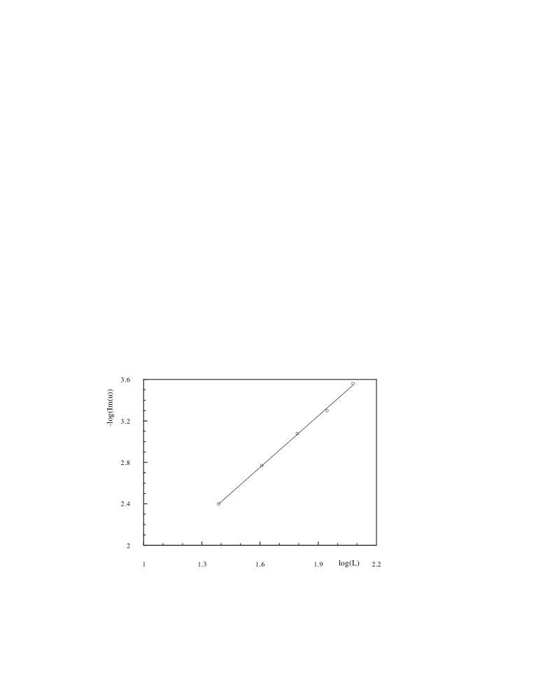
Figure 2: $-\log\mbox{Im}u^{0}_{N}$ versus $\log L$.

The remarkable linearity of the plot denounces a good scaling behavior already for small lattices. From these data (numerical archeology at today, but we are discussing about the method, not about the numbers!) one gets the reasonable estimate $\nu\simeq.620\pm.010$ (the best estimate for $\nu$ at the time of this simulation was the far superior $\nu\simeq.631\pm.001$ by Le Guillou and Zinn-Justin). But with this method, for example, we can get a very straightforward measurement of the ratio of the critical amplitudes (a quantity that is not easy to obtain in the series expansion approach). We measure, as we have discussed before, the angle $\phi$ at which the complex zeroes depart from the real $u$ axis in the infinite volume limit. One has that

$$\tan\left((2-\alpha)\phi\right)=\frac{\cos(\pi\alpha)-\frac{A^{(+)}}{A^{(-)}}}{\sin(\pi\alpha)}\ .$$ (20)

So, for example, in [30] we got an angle of $55.3\pm 1.5$ degrees, and an amplitude ratio of $0.45\pm 0.07$. This is an accurate and reasonable result. The method works!

2.2 Complex Zeroes in a Non-Abelian Four Dimensional Lattice Gauge Theory

In the former section we have described the method one can use to locate complex zeroes of the partition function. We will discuss now the physical problem for which this technique was first introduced by ([11]): I am basically taking this chance to give a ten lines crash course in Lattice Gauge Theories, LGT (that here will mainly be a fancy Statistical Mechanics, constructed by exploiting a powerful symmetry). We will be discussing about locating complex zeroes in a non-abelian $4d$ LGT, i.e. about one of the ways of getting numerical evidence to show that there is no deconfining phase transition in the infinite volume limit. While writing these notes I do not know what will Peter Hasenfratz decide to include in his contribution to this volume ([18]): in any case it will be an interesting reading for the physicist interested to LGT. If in need of more material, you could look at one of the books that are available, [41, 36], to the classical lecture notes by [26], to the Les Houches notes by [37].

In a Lattice Gauge Theory variables leave on links (as opposite to sites for a normal Statistical Mechanics) of a $d$-dimensional lattice (simple cubic, for simplicity, in the following), and we will label them by $U_{\mu}(n)$, where $n$ is a $d$-dimensional site label, and $\mu$ denotes one of the lattice directions (we show the link variable in fig. (3.A)). Different gauge theories are characterized by different kind of variables. In the relevant case of Quantum Chromo Dynamics, the theory of strong interaction of elementary particles, they are $SU(3)$ matrices (here we will consider a simpler theory with many similar features, the one of $SU(2)$ $2\cdot 2$ matrices). In the case of a $SU(M)$ gauge group $U$ is a $M\cdot M$ matrix with $U\cdot U^{\dagger}=1$, and $det(U)=1$.

Figure 3: From gauge variables to Wilson loops. See text.

The Boltzmann equilibrium probability distribution can be written as

$$P_{B}\simeq e^{\beta\sum_{P}U_{P}}\ ,$$ (21)

where the sum runs over all plaquettes (the smallest closed circuits, see (3.B)) of the lattice, and

$$U_{P}\equiv U_{\mu}(n)U_{\nu}(n+\hat{\mu})U^{\dagger}_{\mu}(n+\hat{\nu})U^{\dagger}_{\nu}(n)\ ,$$ (22)

i.e. one takes on each elementary plaquette the product of ordered link matrices (by defining $U_{\mu}(n)=U^{\dagger}_{-\mu}(n+\hat{\mu})$).

This theory has a dramatically large invariance, known as gauge invariance: if we pick up arbitrarily a group element $g(n)$, that we can choose independently on each site, and we transform all the link variables under

$$U_{\mu}(n)\to g(n)U_{\mu}(n)g^{\dagger}(n+\hat{\mu})\ ,$$ (23)

the action of the theory does not change (and do not change all observable quantities, i.e. products of links on closed loops, see (3.C)). In the Ising model the crucial $Z_{2}$ symmetry is only a global symmetry: the theory is symmetric under inversion of all $\sigma(n)$ variables. Here, on the contrary, we have the right to select an independent frame rotation at each lattice point, and the theory does not change. Such gauge symmetry is exact in the lattice theory. This is the crucial step of the Wilson approach to LGT: in the same way in which the $2d$ Ising model Onsager solution is described by Majorana fermions at the critical point, where the correlation length becomes infinite and details of the lattice structure are forgotten, the critical limit of lattice QCD is the usual continuum QCD, the theory of interacting quarks and gluons. The fact that continuum gauge invariant is exactly preserved on the lattice (as opposed, for example, to Lorentz invariance, that is obviously broken by lattice discretization) is a crucial point of the approach.

We have said already, and we will not enter in details, that products of link variables on closed loops are the observable quantities.

We also remark that the inverse temperature $\beta$ that appears in the Boltzmann distribution (21) is connected to the coupling constant of the continuum gauge theory one recovers in the limit of small lattice spacing:

$$\beta_{StM}\simeq g_{GT}^{-2}\ ,\ \ T_{StM}\simeq g_{GT}^{2}\ .$$ (24)

The theory has a phase transition at $T=0$ (here $g\to 0$), where the correlation length diverges (exponentially in $\frac{1}{T^{2}}$). As usual in this continuum limit the lattice structure becomes irrelevant.

For high values of $T$ it is easy to prove the relation we have depicted in (3.D): a Wilson loop (the product of oriented link variables over a closed loop) of large size $R\cdot M$ decays as the exponential of minus the string tension $\sigma$ times the area of the loop in the confined region. If quarks are confined and cannot be separated out from color singlet states (the physical particles, mesons and baryons) we have an area decay of large Wilson loops. So, the nice part is that, as we said, it is easy to prove that Lattice QCD is confined in the high $T$ region (where the theory is very different from the continuum theory). The bad part is that one can prove that for all LGT, including the Lattice QED: since electrons are known to be free in the continuum theory, if everything goes right in this case something will have to happen. What happens for example in the case of QED is that a finite $T$ phase transition separates two regions, the confined, unphysical one, and the deconfined physical theory. One has to show that the same does not happen in Lattice QCD, and that the theory does not undergo a phase transition that would destroy confinement.

Our analysis of lattice zeroes was studying this problem. The technique is exactly the same we have described in the former section. In fig. (4) we draw curves with

$$\mbox{Re}\left(\frac{Z(\eta+i\xi}{Z(\eta)}\right)=0\ ,$$ (25)

and curves with

$$\mbox{Im}\left(\frac{Z(\eta+i\xi}{Z(\eta)}\right)=0$$ (26)

(for the exact curves the reader should consult the original reference, [11]). It is clear from the figure one can determine the zero with good precision. Since one finds a zero quite far from the real $\beta$ axis, and it does not approach the real axis for larger lattice sizes, one does not expect a real phase transition, but is measuring a transient phenomenon that is irrelevant as far as the real continuum limit is concerned. It is clear that the evidence we have discussed here is the same one exploits when using finite size scaling techniques, looking for example at the behavior of a peak of the specific heat. It is interesting that one can directly study the position of complex zeroes of the partition function.

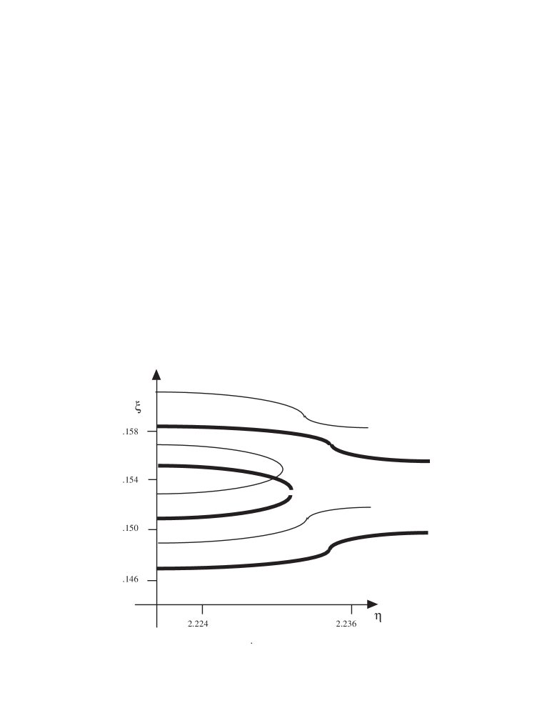
Figure 4: Lines of zeroes of the imaginary part (thin curves) and of the real part (thick curves) of the ratio of partition functions.

2.3 Data Analysis

In equation (12) we have already seen that our approach can be used to deduce information at $\beta$ after running a simulation at ${\tilde{\beta}}$. We can generalize (12) by noticing that we can sample also magnetizations $m$ (so we can reconstruct all moments of $m$). After each measurement we write down the energy and the magnetization of the configuration (that we assume to be at thermal equilibrium). We have that

$$F_{E,m}(\beta,h)=F_{E,m}({\tilde{\beta}},{\tilde{h}})\ \frac{e^{({\tilde{\beta}}-\beta)E+({\tilde{h}}-h)m}}{\sum_{{\tilde{E}},{\tilde{m}}}F_{{\tilde{E}},{\tilde{m}}}({\tilde{\beta}},{\tilde{h}})e^{({\tilde{\beta}}-\beta)E+({\tilde{h}}-h)m}}\ .$$ (27)

In [13] one finds a very nice picture showing how well the method can work for example for the case of the $2d$ Ising model.

The method we have described here is very useful, for example, when one wants to measure the finite size scaling behavior of physical observable quantities. Let us consider for example the specific heat $C_{V}$. The maximum value $C_{V}$ takes on a finite lattice of linear size $L$, $C_{V}^{\max}(L)$ scales at a critical point as

$$C_{V}^{\max}(L)\simeq L^{\frac{\alpha}{\nu}}\ .$$ (28)

The main problem is in the fact that we only measure for a discrete set of values of the temperature $T$ (by normal MC or by using a $T$-changing Monte Carlo procedure, see later in this notes). A priori we do not know at which value of $T$ on a given lattice the specific heat takes its maximum value, and such $T$ value depends on $L$:

$$T^{\max}(L)\ |\ C_{V}(T^{\max}(L),L)\equiv C_{V}^{\max}(L)\ \mbox{depends on}\ L\ .$$ (29)

It can be difficult to find the correct value of $T^{\max}(L)$: it is a delicate fine tuning process that has to be repeated for each different $L$ value. A wrong determination of $T^{\max}(L)$ can generate a very misleading effect. Let us look at figure (5). The empty dots represent (gedanken) measurements of the specific heat taken with a linear size $L$, at the set of $T$ values which appear in the figure. The filled dots are measurements on a lattice of larger linear size $L^{\prime}$, taken at the same $T$ values. One would assume that the finite size scaling behavior is given by the scaling of the two measured points with higher value of $C_{V}$. But maybe the real maximum, on the larger lattice, is where the triangle is: there the scaling could be very different from the one we found on the points we measured, but sadly we did not measure on this point. We want to stress that this effect creates real practical problems in numerical simulations.

Figure 5: The specific heat versus $T$ for a typical finite size scaling study suffering of troubles that can be cured by reweighting. Empty dots are for the smaller lattice, filled dots for the larger lattice, and the triangle for the point we did not measure and we should have measured.

The pattern of data analysis we have discussed here solves this important problem. Statistical error can be kept under control (by using for example jack-knife and binning techniques), and numerical studies of scaling become (without further computational expenses, since we already had the information) a real quantitative tool.

2.4 Multi-Hystogramming

The idea of reweighting can be pushed forward. [14] introduced the multi-hystogramming. The crucial step is to realize that you can patch data from different simulations at different $\beta_{k}$ values to reconstruct all of the relevant $\beta$ region.

So, we have to sum up histograms. The delicate point is how to sum them up, i.e. how to determine the weights to use in constructing linear combinations of the different entries. The way discussed in [14] is to determine the weights by minimizing the statistical uncertainty over the final estimate for $P_{\beta}(E)$. Let us call $N_{k}(E)$ the data histogram for the $k$-th Monte Carlo run, at $\beta_{k}$. Let us define $\theta_{k}\equiv 1+2\tau_{k}$, where $\tau_{k}$ is the estimated correlation time at $\beta_{k}$, and $n_{k}$ the number of sweeps used in the $k$-th Monte Carlo run. One finds that the parameters $\{g_{n}\}$ can be determined self-consistently by iteration from

$$P_{\beta}(E) = \frac{\sum_{k=1}^{R}\ N_{k}(E)\ e^{\beta_{k}E}\ \theta_{k}^{-1}}{\sum_{j=1}^{R}\ n_{j}\ e^{\beta_{k}E-g_{j}}\ \theta_{k}^{-1}}\ ;$$

$$e^{g_{j}} = \sum_{E}P_{\beta}(E)\ .$$ (30)

We have denoted by $R$ the number of Monte Carlo runs. The method works well, and at today it can be considered as a standard analysis tool.

3 Improved Monte Carlo Methods

We will discuss here about improving Monte Carlo methods. We will be mainly talking about tempering, by [31] (see section (3.1)), where you add a second Markov chain to the usual Metropolis chain: you let $\beta$ vary, trying in this way to make easier for the system to move across deep free energy valleys separated by high free energy barriers. We will also try to discuss about general issues like thermalization, that are of crucial importance already when discussing simple Monte Carlo methods, and that turn out to be even more delicate issues here.

Eventually one is looking for a very effective, very simple simulation method. Somehow when you start the numerical study of a statistical system you work at two different levels. At first you run a quick and not very clean Monte Carlo, to understand the first physics ideas. Only after that you set up complex simulational procedures, data analysis, error determination. It would be nice if the first phase we have just describe could already be based on something more powerful that the usual Metropolis approach: I hope the reader will be convinced that maybe the Parallel Tempering approach (see section (3.3)) is the good candidate for this role. In Parallel Tempering there are no parameters to be tuned, no difficult choices to be done (but for the selection of a set of $T$ values that can be done with some large freedom): it looks like the good thing.

3.1 Simulated Tempering

We will introduce here Simulated Tempering, [31], an improved Monte Carlo method that turns out for example to be very effective for simulating spin glasses (for further studies and applications of tempering see [12, 10, 48, 24, 8]). Later on we will discuss about Parallel Tempering, [44, 15, 20, 19], that turns out to be a better and simpler method (having at the same time these two advantages is a quite rare and appreciated feature). So we will discuss now some complex matter that we will eventually not need in the practical implementation of the method: we will do that since it helps in understanding some of the physical mechanisms that govern the scheme. These mechanisms are common to the most promising parallel tempering scheme. Parameter tuning is not needed in parallel tempering.

Simulated tempering is a global optimization method: it can be seen as an annealing, generalized to $T\neq 0$, with a built-in scheduling. This can be of large practical importance, since setting up the schedule is one of the most difficult and time taking parts of an annealing simulation. Tempering is very similar to annealing, but after the initial thermalization period the field configuration is always at Boltzmann equilibrium at one of the allowed $\beta$ values. This phrase, that is a bit mysterious at this point, is important, and will be clarified in the following.

There are many related techniques, strictly connected methods and needed introductive material. In first one needs to know about generalities of Monte Carlo methods (see for example the lectures in this book by [29]). Theory of multiple Markov chains is the mathematical basis one needs to clarify the theoretical aspects of the method ([44, 15, 20, 19]).

Strictly related to tempering are the scaling approaches based on Umbrella Sampling, [45, 46, 16, 47]: we have already discussed the issue when illustrating data analysis reconstruction. It has to be noticed that many of the ideas we are applying now to numerical Statistical Mechanics and Euclidean Statistical Field Theory have been elaborated many years ago in the context of physics of liquids and of Molecular Dynamics.

Multicanonical Approaches by [4, 5, 2, 3] are also strictly related to tempering, and we will also discuss about them in the following. Multicanonical methods are more ambitious and in many situations potentially more powerful than tempering (but they are a bit more complex): they can try and deal with first order phase transitions, that is not something you want to do with tempering (that works well for continuous phase transitions). We also note that different kind of tempering-like approaches have been proposed, for example in [25].

As we have discussed from the start of these notes Tempering has been built on reconstruction methods, [11, 30, 13, 14]: if we can use data at ${\tilde{\beta}}$ for learning about expectation values at $\beta$ maybe we can also use this information for speeding up the dynamics itself (again, see [29] for an introduction to Monte Carlo simulations and Markov chains). When you run a long simulation you could know much more than you believe (or much less, but we will discuss about that when talking about thermalization and correlation times).

Let us start with describing Simulated Tempering. We want to equilibrate our statistical system with respect to the Boltzmann distribution

$$P(\{\sigma\})\simeq e^{-\beta S(\{\sigma\})}\ .$$ (31)

We choose a new probability distribution, with an enlarged number of variables:

$${\tilde{P}}(\{\sigma\},\{\Sigma\})\ ,$$ (32)

such that, for each given choice of the $\{\Sigma\}$, ${\tilde{P}}$ is Boltzmann with some given choice of $\beta$. We will allow $\beta$ to become a dynamical variable:

$$\{\sigma\}\ \to\ (\{\sigma\},\{\beta_{\alpha}\})\ ,$$ (33)

$\alpha=1,\ \ldots,\ A$. We have allowed $A$ fixed values for the $\beta_{\alpha}$ variables.

The mechanism we are introducing is very simple: the new equilibrium probability distribution is

$$P_{eq}(\{\sigma\},\{\beta_{\alpha}\})\simeq e^{-\beta_{\alpha}H(\{\sigma\})+g_{\alpha}}\ ,$$ (34)

where $H$ is the original Hamiltonian of the problem. The $g_{\alpha}$ are constant quantities, whose meaning will be elucidated in the following. They have to be fine tuned before running the equilibrium sampling, and they only depend on the value of $\alpha$ (only one $g_{\alpha}$ is allowed for each $\beta_{\alpha}$ value).

The probability of finding a given value of $\alpha$ (i.e. the probability for a given $\beta_{\alpha}$ value to occur during the run) is:

$$P_{\alpha}=z_{\alpha}e^{g_{\alpha}}\equiv e^{g_{\alpha}-\beta_{\alpha}f_{\alpha}}\ ,$$ (35)

where $z_{\alpha}$ is the partition function at fixed $\beta_{\alpha}$,

$$\int\{d\sigma\}e^{-\beta_{\alpha}H(\{\sigma\})}\ ,$$ (36)

and $f_{\alpha}$ is the free energy of the system with fixed $\beta_{\alpha}$. (35) shows that the free parameters $g_{\alpha}$ are connected to the free energy of the system. For making the probability of different $\beta$ values to occur to be equal (i.e. the system to visit with the same frequency all allowed $\beta$ values) we need to set

$$g_{\alpha}=\beta_{\alpha}f_{\alpha}\ .$$ (37)

Since we do not know th $f_{\alpha}$ that will amount to use for the $g$’s the best available estimate for $f$. We will discuss in the following how to produce a good guess for the $g_{\alpha}$, that can also be improved systematically. Since eventually parallel tempering will not need any kind of parameters to be fine tuned we will not go in details about this issue (explaining what the $g$ are in simple tempering is useful for reaching a better physical understanding of both tempering and parallel tempering).

If we are mainly interested in studying the system at $T={\tilde{T}}$ we will allow for a set of $T_{\alpha}$, for example at constant distance, $T_{0}\equiv{\tilde{T}}$, $T_{1}\equiv({\tilde{T}}+\delta)$, $T_{2}\equiv({\tilde{T}}+2\delta)$, $\ldots$ (see figure (6)). We will discuss how to select optimal values for $\delta$ (this has to be done also in parallel tempering, but one does not need fine tuning). After the runs if you want you can use reconstruction schemes to use all of the information contained in all samples, but in this kind of approach this is typically not necessary (since we are looking for thermalized configurations in a complex, cold broken phase, and the main information is typically contained in the $T_{0}$ data).

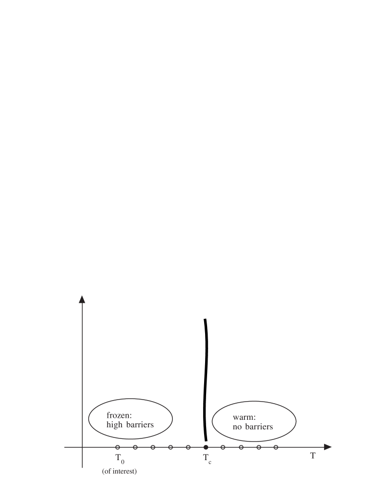
Figure 6: The choice of the $T$ values to be used in the tempered simulation of a complex system.

The main physical ideas are

1. The system is frozen at low $T$. High energy barriers separate different free energy valleys.

2. When the system warms up during tempering the free energy barriers get smaller. They disappear when the system crosses $T_{c}$.

3. When it cools down again it will probably explore a different local minimum.

The method seems to work nicely for second order like phase transitions: for that to happen you need the broken state to be conformationally similar to the high $T$ one.

We will now analyze in detail a full updating sweep, in order to make the procedure clear.

1) Sweep the full lattice, maybe $s$ times ($s>1$ could help) and run a full normal Monte Carlo (Metropolis, or cluster, or over-relaxed or what you like better) update for the $\{\sigma\}$ variables at fixed $\beta_{\alpha}$.

2) Propose the update

$$\beta_{\alpha}\to\beta_{\alpha^{\prime}}\ ,$$ (38)

where $\alpha^{\prime}=\alpha\pm 1$ with probability $\frac{1}{2}$ (at $\alpha=1$ and $\alpha=A$ we can or not decide not to move with probability $\frac{1}{2}$, since we are not interested in detailed balance in $\beta$ space: see [29] about the importance of rejected moves).

We accept the update with normal Metropolis weight. Here the factor in the exponential only changes because of the change in $\beta$, since the configuration energy does not change:

$$\Delta S_{\mbox{tempering}}=(\beta_{\alpha^{\prime}}-\beta_{\alpha})H(\{\sigma\})+(g_{\alpha^{\prime}}-g_{\alpha})\ ,$$ (39)

where both the $H$ and the $(g_{\alpha^{\prime}}-g_{\alpha})$ terms are constant. If $\Delta S<=0$ we accept the $\beta$ update, if $\Delta S>0$ we accept it if a random number uniformly distributed in $(0,1)$ is smaller than $e^{-\Delta S}$.

A good first guess for the $g_{\alpha}$ can be deduced from (39) (then, as we said, the $g$’s can be systematically improved). We can take the $g$ such that in average $\Delta S$ is balanced:

$$(g_{\alpha^{\prime}}-g_{\alpha})=-(\beta_{\alpha^{\prime}}-\beta_{\alpha})\frac{\langle H\rangle_{\beta_{\alpha}}+\langle H\rangle_{\beta_{\alpha^{\prime}}}}{2}\ ,$$ (40)

that holds at first order in $\delta\beta$. We see that the $g$, by balancing for the free energy of the system, do not allow the system to follow in the lowest energy state and stay there forever. The first correction is of the form

$$C_{V}^{\alpha}(\delta\beta)^{2}\ ,$$ (41)

and keeping this term of order one implies that in the large volume limit $\delta\beta$ has to be kept of order $C_{V}^{-\frac{1}{2}}$, see also later.

Now the crucial observation: at each $\beta_{\alpha}$ value (after the initial thermalization) the system is always in equilibrium with respect to the usual Boltzmann distribution. The system is all the time (even at the moment of $\beta$-transitions) at thermal equilibrium.

The analysis of observable quantities is very easy. One just has to select all configurations which were flagged by a given $\beta$ value:

$$\langle O\rangle_{\beta_{\alpha}}=\frac{\sum_{\mbox{All configurations at}\beta_{\alpha}}O_{\mbox{conf}}}{\mbox{Number of configurations at}\beta_{\alpha}}\ .$$ (42)

How do we select a good set of $\{\beta_{\alpha}\}$ values? Fig. (7) can help to give an idea. Let the first $P(E)$ on the left be the one at the lowest $T$ value (the one we are interested in thermalizing). The center the one is at $T+\delta$, i.e. at the second $T_{\alpha}$ value. We request that the overlap of the two probability distributions is non-negligible. A configuration with an energy included in the colored region of the picture is typically a good configuration both at $T$ and at $T+\delta$ (it is here that problems connected to discontinuities, like in first order phase transitions make the method fail). So, $\delta\equiv T_{\alpha+1}-T_{\alpha}$ has to be selected such that there is a non-zero overlap among the two energy probability distributions (as usual in Metropolis like methods that is connected to having a reasonable acceptance factor, of order $0.5$, for the $\beta_{\alpha}$ moves). That should also make more clear why we could like to do more than one $\{\sigma\}$ sweeps before updating $\beta$: we want to avoid a series of jumps between adjacent $\beta_{\alpha}$ values, and give to the system the possibility of moving at fixed $\beta$ at the opposite extremum of the $P(E)$ before trying changing $\beta$ again.

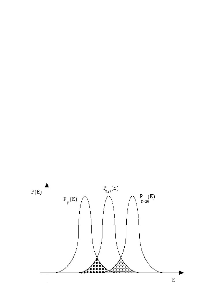
Figure 7: $P(E)$ for different values of $T$.

We repeat which are the basis of the physical mechanism we are interested in. We are thinking about systems with very high free energy barriers. Warming the system up lowers the barriers, which disappear at $T_{c}$. When cooling down (always staying at thermal equilibrium!) the system can fall in a completely new valley.

Experimentally the method turns out to work very well for $3d$ Edwards-Anderson spin glasses. It is interesting to note that temperature chaos, [27, 28, 39], should give troubles, but on the lattice sizes we have been able to study we did not get them: it is interesting to try and understand more about this issue. In the case of $3d$ Edwards-Anderson spin glasses by using parallel tempering (see (3.3)) we have been able to thermalize a $16^{3}$ system down to $0.7T_{c}$ ([33]). On a $24^{3}$ lattice one is able to thermalize with a reasonable computer time (we are talking about single runs on one disorder sample taking order of one day of workstation) down to $0.9T_{c}$, while for lower $T$ the situation gets more difficult to control.

The method does not work, [22], for generic heteropolymers (with order $30$ sites, Lennard-Jones potential with quenched random couplings [21]), and this is probably connected to the fact that the glassy transition is in this case of a discontinuous nature: for true (small) proteins, on the contrary, the method seems to be helpful [17]. Also the method has been applied among others ([12, 8]) by [10] to the $4d$ disordered Heisemberg model, by [24] to the $2d$ EA spin glass (by noticing one of the important advantages of the method, i.e. the trivial vectorization and parallelization of the scheme), and by [48] to $CP^{N-1}$ models.

3.2 Random Field Ising Model

The case study we have done in our first tempering paper, [31], was discussing the Random Field Ising Model, and it is ideal to illustrate in some more detail the main feature of the method: we will discuss it here. The model is defined by the Hamiltonian

$$H=-\sum_{\langle i,j\rangle}\sigma_{i}\sigma_{j}+\sum_{i}h_{i}\sigma_{i}\ ,$$ (43)

where $\sigma_{i}=\pm 1$, the sum with two indices runs over first neighboring sites on a simple cubic lattice in $d$ dimensions, and the local external fields $h_{i}$ are quenched random variables, which take the value $\pm|h|$ with equal probability.

We have taken $d=3$, $V=10^{3}$ sites and $|h|=1$, sitting close to the critical region, on the cold side (we will focus here on studying $\beta=.26$). Fig. (8) gives an idea about the critical region. The specific heat has a maximum close to $\beta=.25$. In these first runs in most cases we allowed the system to visit only $3$ $\beta$ values, ($\beta_{\alpha}$ $=$ $(.24,.25,.26)$), and sometimes $5$ $\beta$ values: for the Edwards Anderson model in the most recent runs of [33] on a $24^{3}$ lattice we use up to $50$ $\beta$ values. The $3$ $\beta$ values we have given above are selected such to span from the cold phase to the warm phase. This is the general principle: the system has to be allowed to travel, in $\beta$ space, from the cold phase, that has a physical interest, to the warm phase, where free energy barriers disappear and correlation times are short.

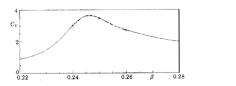
Figure 8: The measured specific heat $C_{V}$ as a function of $\beta$. $\beta=0.26$, in the cold region, is the point on which we focus.

In fig. (9) we plot the $\beta_{\alpha}$ values the system selects in the course of the dynamics. Notice that the system is not getting trapped in the cold or in the warm phase: acceptance of the $\beta$ swap is easy, and the system easily travels among the two phases.

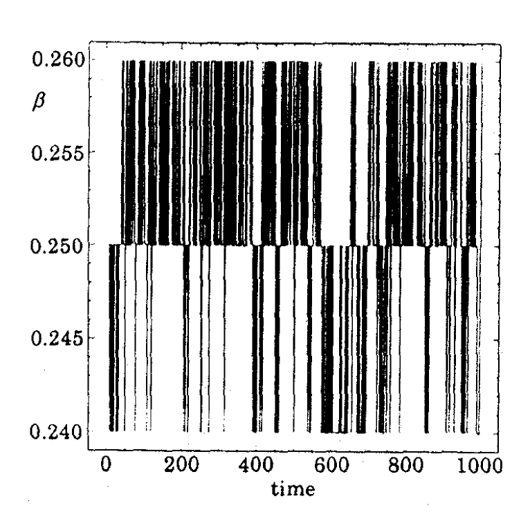
Figure 9: $\beta_{\alpha}$ as a function of the Monte Carlo tempering time.

The magnetization measured from a typical normal, fixed $\beta$ Monte Carlo metropolis runs is shown in fig. (10): here the correlation time, since one never sees a flip to the opposite magnetization time, seems short. That taking fig. (10) at face values would be misleading is clear from the magnetizations from a tempering run shown in fig. (11): here tempering is allowing the system to flip among the $\pm m$ states, and it is clear that configurations with positive $m$ have a relevant weight in the equilibrium distribution.

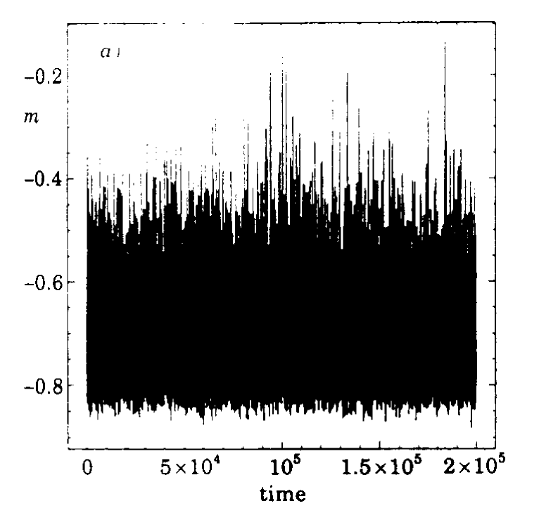
Figure 10: Magnetization as a function of Monte Carlo time, at $\beta=0.26$, for normal Metropolis algorithm. The system never tunnels to a positive magnetization value.

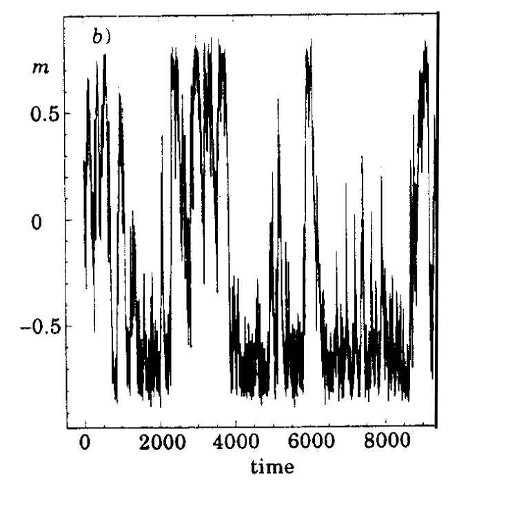
Figure 11: Magnetization versus Monte Carlo time for tempering. Here all $\beta$ values are included: the measured magnetization are related to configurations that are at Boltzmann thermal equilibrium with different temperature values.

In fig. (12) we plot the magnetization of the configurations that got a $\beta$ value of $0.26$. Here one clearly sees that the state with positive $m$ is allowed at $\beta=0.26$ with a probability smaller than for the negative $m$ state but definitely non-zero. These last figures give the main idea. In a non-disordered Ising model flipping from the minus state to the plus state would be irrelevant, if we are not interested in studying details of the tunneling dynamics: we know by symmetry that to the minus state corresponds an identical plus state. But this is not true for a disordered model, where on the contrary the tunnel among degenerate ground states that are not related by a trivial symmetry is the most interesting part of the dynamics. Here the random quenched magnetic field breaks the symmetry, and we want to explore the different ground state. Tempering allows us to do that.

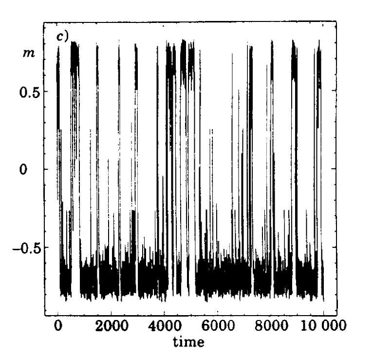
Figure 12: As in fig. (11), but we have selected only configurations with $\beta=0.26$.

This was a very easy numerical experiments, but the steps we have described characterize also a more complex settings: for example we already told that the numerical simulations we are running now ([33]) on large lattices for the $3d$ Edwards Anderson spin glass are quite complex (but they work very well).

Tempering is related to annealing. A trivial extension of annealing to non-zero values of $T$ is impossible: annealing gives only information about energy, while for $T>0$ we want to deal with the free energy. We do not get from annealing any information about the entropic structure of the phase space. Tempering can be seen as such a generalization.

Tempering could also turn out to be an effective global optimization scheme, even if this issue has non been looking in much detail until now. Very preliminary unpublished studies are by [40, 43]. The most important point is that tempering contains a built-in, self-implemented schedule. Setting up the schedule is the most serious problem with annealing, and tempering does it for us.

3.3 Parallel Tempering

Parallel Tempering has been discussed by [44, 15, 20, 19]. We will describe it here. As we already said it is so simple that makes many of the details we have discussed with tempering only informational (we look at that as a plus). Also, the parallel tempering performs dramatically well, for example, on finite dimensional Edwards Anderson models.

In figures (6) and (7) we have shown how we select the $T$ values we use during the simulation. Let us say that by using the criteria we have defined before we need for example $N_{(\beta)}$ values of $\beta_{\alpha}$. Now in the parallel tempering approach, you run $N_{(\beta)}$ simulations in parallel ( $N_{(\beta)}$ different configurations $C_{\alpha}$ of the system that evolve in the same quenched disordered landscape). Each copy starts with assigned a different $\beta$ values. For example start with

$$\beta(C_{0})=\beta_{0};\ \beta(C_{1})=\beta_{1};\ \ldots\ \beta(C_{\alpha})=\beta_{\alpha};\ \ldots\ \beta(C_{N_{(\beta)}})=\beta_{N_{(\beta)}}\ .$$ (44)

Now the composite Monte Carlo method is based on two series of steps:

1. Update the $N_{(\beta)}$ copies of the system with an usual Metropolis sweep of

   $$\left\{\sigma\right\}_{C_{\alpha}}\ldots\left\{\sigma\right\}_{C_{N_{(\beta)}}}\ .$$ (45)

2. Swap the $\beta$ values.

   • Propose the first $\beta$-swap: the configuration that is at $\beta_{0}$ can go to $\beta_{1}$ and that one that is at $\beta_{1}$ can go at $\beta_{0}$. Each spin configuration carries a $\beta$-label. Configurations carrying adjacent $\beta$-labels try to swap their labels. You use Metropolis for swapping $\beta$ with the correct probability (see later).

   • Propose the second $\beta$-swap: the configuration that is at $\beta_{1}$ can go to $\beta_{2}$ and that one that is at $\beta_{2}$ can go at $\beta_{1}$.

   • And so on, to the last couple of configurations: the configuration that is at $\beta_{N_{(\beta)}}$ can go to $\beta_{N_{(\beta)}-1}$ and that one that is at $\beta_{N_{(\beta)}-1}$ can go at $\beta_{N_{(\beta)}}$ .

I stress the fact that you always try to swap adjacent $\beta$-values (or the procedure would be not effective). At a given point in time configuration number $27$ can be at $\beta_{0}$ and configuration number $3$ at $\beta_{1}$: these are the two configurations you will try to swap.

The $\beta$-Metropolis swap: as usual, you will accept if the swap makes the energy decreasing, and will accept with probability $e^{-\Delta S}$ if it makes the energy increasing. You will have to compute

$$\Delta S = S^{\prime}-S$$

$$= (\beta_{\alpha+1}E_{C_{\beta_{\alpha}}}+\beta_{\alpha}E_{C_{\beta_{\alpha+1}}})-(\beta_{\alpha}E_{C_{\beta_{\alpha}}}+\beta_{\alpha+1}E_{C_{\beta_{\alpha+1}}})\ ,$$

where obviously $E_{C_{\beta_{\alpha}}}$ and $E_{C_{\beta_{\alpha+1}}}$ do not change during the $\beta$-swap.

Here there is no freedom (and no need) for an additive term like the one we had before, $g_{\alpha}$. In this method once fixed the $\beta$ values (the fixing of the $\beta$ can be done loosely, and does not need fine tuning) there are no free parameters, and no fine tuning needed. The ensemble of the parallel tempering is very different from the one of tempering, even if the two methods look very similar.

A possible way to look at the fact that we do not need the $g$ parameters is the following. The $g_{\alpha}$ were needed in order to prevent the system from collapsing to the state with lowest energy. But here there is a fixed number of $\beta$-values. A given value of $\beta_{\alpha}$, for example $\beta_{23}$, cannot disappear. This fact makes things easy for us.

3.4 The Thermalization

Thermalization is a crucial issue. This is already true for usual spin models and usual local dynamics. We want to be sure that we are looking at a system that has reached equilibrium, and after that we want to be sure we have correlation times under control. In other words we are interested in studying the asymptotic equilibrium probability distribution, and we need to be sure that we are collecting the right information. In complex dynamics like tempering, involving multiple Markov chains, it is even more difficult to keep correlation times under control. The fact that we are typically studying complex systems, where slow dynamics is one of the most prominent feature, does not help. I will discuss here some details of the understanding we have reached about this issue. We will try to understand which kind of thermalization criteria we can adopt when using tempering.

Let us start by describing what happens when we use a simple Metropolis dynamics for studying a system with quenched disorder. Here we will not give details, that can be found for example in [35], but I will only remind the reader that in this case one mainly deals with functions of the overlap

$$q^{\alpha\beta}\equiv\frac{1}{V}\sum_{i}\left(\sigma_{i}^{\alpha}\sigma_{i}^{\beta}\right)\ ,$$ (47)

where $\alpha$ and $\beta$ label two replica’s of the systems, i.e. two equilibrium configurations defined under the same realization of the quenched disorder. The overlap gives us information about how similar are two typical equilibrium configurations of the same system. $q$ plays the role of the order parameter, and it is the equivalent of the magnetization $m$ for usual spin models. The typical shape of the probability distribution of $q$, averaged over the quenched disorder $J$ (see [35]), is shown in fig. (13). The two peaks would be sharp (at $\pm m^{2}$) for an usual spin model. The non-trivial part here is the fact that there is a continuous, non-zero contribution close to $q\simeq 0$: the system can exist at equilibrium in many states, that can even be, in the infinite volume limit, completely different. The non-trivial part here is the fact that there is a continuous, non-zero contribution close to $q\simeq 0$: the system can exist at equilibrium in many states, that can even be, in the infinite volume limit, completely different.

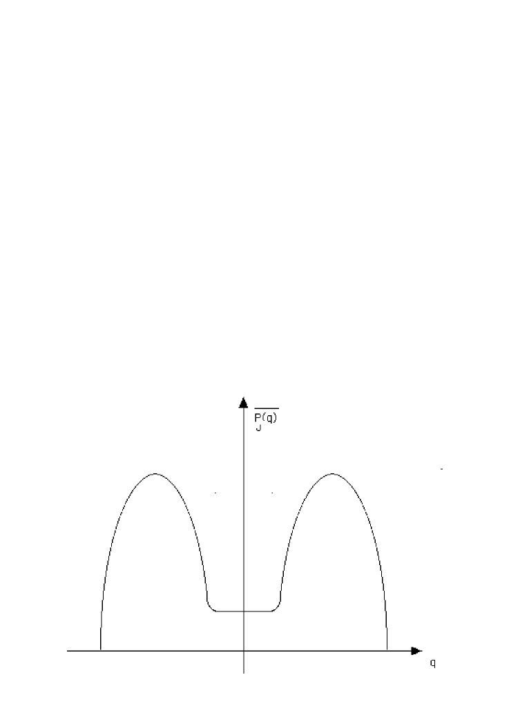
Figure 13: $\overline{P_{J}(q)}$ versus $q$. The flat part close to $q=0$ is the most remarkable feature of the behavior of a class of disordered systems.

In the case of a normal Metropolis update one can use two very strong criteria to check thermalization.

1. Check symmetry of $P(q)$ under $q\leftrightarrow-q$ for each sample. This is a very strong criterion. The main issue is here that the full flip of the whole system, $\{\sigma\}\to\{-\sigma\}$ is the slowest mode of the dynamics. If you have done that well enough to get a good $\pm\sigma$ symmetry you have explored the whole phase space. In the simulation of a normal spin-model in the cold phase we would never be so demanding (if not interested to details of tunneling amplitudes): we would just seat in one vacuum and compute observable quantities there. As we already said, this is the main difficulty connected to the study of disordered systems.

   In fig. (14) we give two typical $P(q)$ for two different given quenched realizations of the disorder. In the Parisi solution of the mean field (see [35]) you can detailed compute many properties: for example how many configurations contribute to the $q\simeq 0$ plateau. The numerical results in $3d$ show a very good similarity with the mean field results ([32, 33]).

   This criterion can be adopted for tempering, but in this case it is not so strong anymore: in tempering methods the mode $\{\sigma\}\to\{-\sigma\}$ is not necessarily a very slow mode. It is possible in this case that one gets a very symmetric $P(q)$ that is not related to the asymptotic equilibrium distribution function.

2. A second criterion, originally due to [7], that is very strong for usual dynamics, is based on using two different definitions of the $P(q)$.

   1. After a random start from two different spin configurations simulate two independent copies of the system (in the same set of $\{J\}$ couplings). This is the definition we had in mind till now. If we denote by $\sigma$ and $\tau$ the two copies of the system we call $q_{2}$

      $$q_{2}\equiv\frac{1}{V}\sum_{i}(\sigma_{i}\tau_{i})\ ,$$ (48)

      and $P_{2}(q)$ the equilibrium probability distribution of $q_{2}$.

   2. In the second approach we use a dynamical measurement, at different times. We wait for a large Monte Carlo time separation $t$ and we define (for $t_{0}$ large enough)

      $$q_{dyn}\equiv\frac{1}{V}\sum_{i}\left(\sigma_{i}(t_{0})\sigma_{i}(t_{0}+t)\right)\ ,$$ (49)

      where eventually we will take an average over $t_{0}$. We define $P_{dyn}(q)$ the equilibrium probability distribution of $q_{dyn}$.

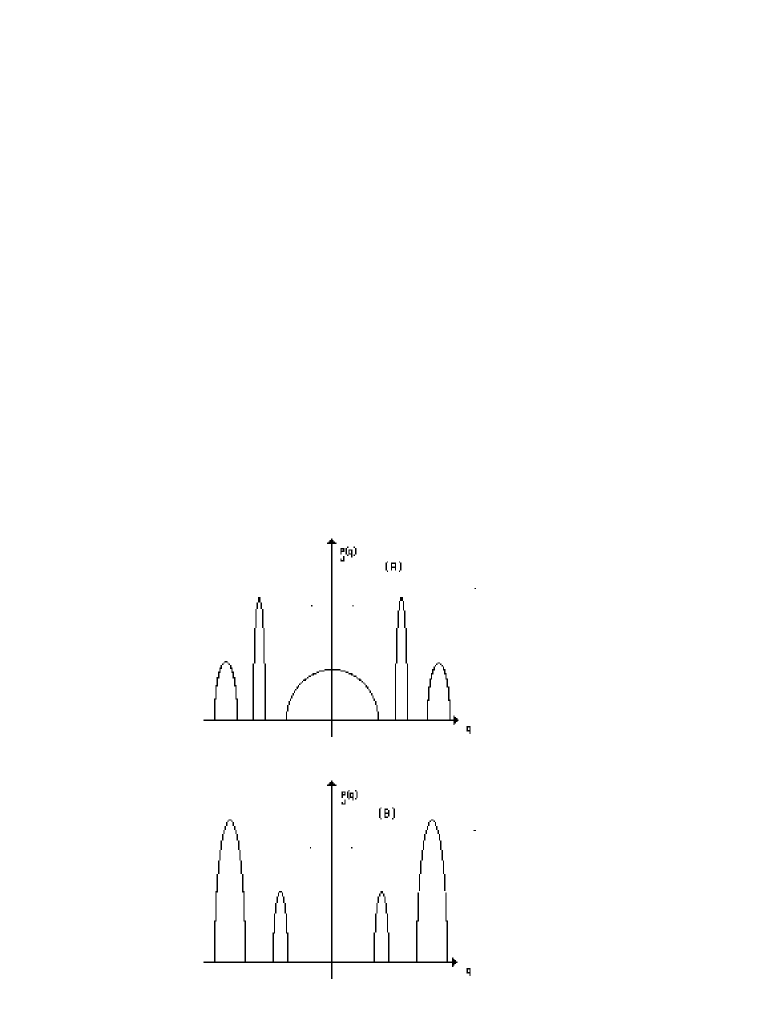
Figure 14: Two typical $P_{J}(q)$ versus $q$, for two different realizations of the coupling.

When using the first definition at short times the two copies are not as similar as they will be asymptotically. Correlations only build up slowly. So $P_{2}(q)\to P(q)$ from below, and at short times $P_{2}(q)$ is centered at lower $q$ values than $P(q)$. On the contrary at short times $\sigma(t_{0})$ and $\sigma(t_{0}+t)$ are correlated, i.e. $q_{dyn}$ at short times tends to be larger than the asymptotic value. So $P_{dyn}(q)\to P(q)$ from above. Only for times large enough $P_{dyn}(q)=P_{2}(q)$, and we use this condition to check thermalization.

Also the extension of this second criterion to tempering is not straightforward, since now dynamics is assigning to different configurations different $\beta$ values.

For parallel tempering runs, for example, we use three main conditions to check thermalization.

1. We check that all observables are not drifting in time. We look for example at the energy $E$ and at $q^{2}$. We check, on logarithmic time scales, that they have safely converged to a stable value. We also explicitly look at the full $P_{J}(q)$, and check it has no drift.

2. We check that the spacing of the allowed $\beta_{\alpha}$ is small enough to guarantee a good acceptance ratio for the proposed $\beta$ swaps.

3. We demand that each of the $N_{(\beta)}$ configurations $C_{\alpha}$ must have visited each of the allowed $\beta_{\alpha}$ values with similar frequency. If we have done ten millions sweeps and we have ten allowed $\beta$ values we demand that each configurations has spend more or less one million sweeps in each $\beta$ value. We keep a set of counters to check that. We want to be able to detect situations where some systems are confined in a part of the phase space, and a good acceptance factor is not enough to avoid that (the configurations could just be flipping locally in $\beta$ space).

3.5 More Comments

It is interesting to note some other technical comments about tempering like methods, mainly thinking about the large volume scaling behavior and about the performances of the method. Here we go, with a slightly miscellaneous series of comments.

When you increase the lattice size you need a larger number of allowed $\beta_{\alpha}$ values, i.e. a larger $N_{(\beta)}$, to sample the $\beta$-space, and to reach the region where free energy barriers disappear. The method is critically slowed down, but only like a power law.

Again, disordered systems need more attention than normal systems. You have to check that for each realization of the quenched disorder $\{J\}$ the condition that all $C_{\alpha}$ have visited all $\beta_{\alpha}$ values for similar periods of time is satisfied. From our experience the situation seems quite sharp: when the method works it works well, when it does not work it is a disaster (i.e. some visiting times are of order zero and some are of the order of the total time). For normal tempering (but parallel tempering seems preferable in all known cases) the constants $\{g_{\alpha}\}$ have to be tuned separately in each sample.

Let us discuss in better detail about volume scaling in tempering like methods. Let select the allowed $\beta$ values at a constant distance $\delta$:

$$\beta_{\alpha+1}=\beta_{\alpha}+\delta\ .$$ (50)

The probability for accepting a $\beta$-swap is

$$P_{SWAP}(\beta_{\alpha},\beta_{\alpha+1})\equiv e^{-\Delta}\ ,$$ (51)

and

$$-\log(P_{SWAP})=\Delta=\delta\cdot\left(S(C_{\beta_{\alpha+1}})-S(C_{\beta_{\alpha}})\right)\simeq\delta^{2}\frac{dE}{d\beta}\ .$$ (52)

So if the specific heat is not diverging we want to select

$$\delta^{2}N=\mbox{constant}\ ,\ \delta\simeq N^{-\frac{1}{2}}\ ,\ \mbox{i.e.}\ N_{\beta}\simeq N^{\frac{1}{2}}\ .$$ (53)

At a second order phase transition point, where the specific heat diverges, we have to be slightly more careful, since the number of intervals we need turns out to be higher. One has

$$\xi \simeq|T-T_{c}|^{-\nu}\ ,\ C_{V}\simeq|T-T_{c}|^{-\alpha}\ ,$$ (54)

$$|T-T_{c}| \simeq\xi^{-\frac{1}{\nu}}\simeq N^{\frac{1}{d\nu}}\ ,$$

$$C_{V} \simeq N^{\frac{\alpha}{d\nu}}\ .$$

So we get

$$\delta^{2}N^{1+\frac{\alpha}{d\nu}}=\mbox{constant}\ ,\ N_{\beta}\simeq\delta^{-1}\simeq N^{\frac{1}{2}(1+\frac{\alpha}{d\nu})}\ ,$$ (55)

that is our final estimate.

The choice of the set $\{\beta_{\alpha}\}$ is not crucial (not like the $g_{\alpha}$’s in the serial tempering). We can select the same set for all the realizations of the disorder, paying only the price of loosing some small amount of efficiency.

In fig. (15) we sketch (the picture only has a pictorial role) the correlation times computed by [19]. Filled dots are for tempering, empty dots for multicanonical. Simulations are for a $3d$ Edwards Anderson spin glass, with couplings $J=\pm 1$. $32$ $\beta$ values have been allowed in the parallel tempering run, for all $N$ values. $\tau$ is defined as the typical time needed from a spin configuration for going from the cold to the warm phase. It is worth noticing that in the parallel tempering, given the $\beta$ set, there are no parameters to be fixed.

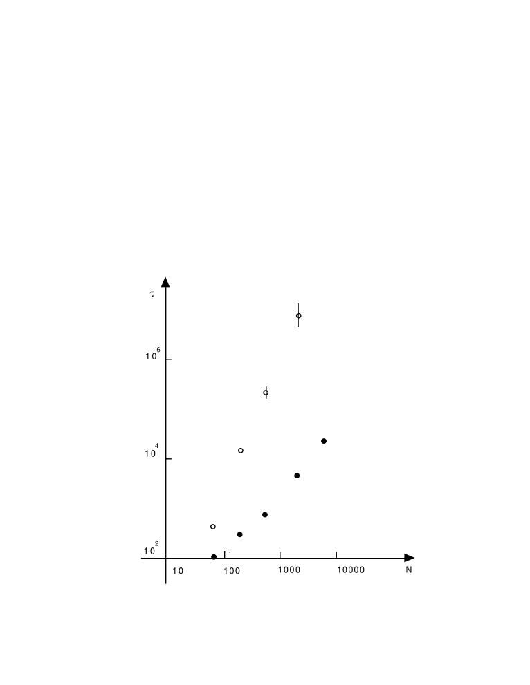
Figure 15: Correlation times for multicanonical and for tempering, for different lattice sizes (in log-log scale). The figure is only sketchy, and the interested reader can find the exact data point in fig. 2 the original paper by [19]. Filled dots are for tempering, empty dots for multicanonical.

3.6 Umbrella Sampling and Reweighting

All the idea we have discussed up to now are related to the technique of Umbrella Sampling by [45, 46] (mainly developed for simulations of liquid systems). Let us show now how we can relate that to reweighting techniques.

We consider an observable quantity $A$

$$\langle A\rangle_{\beta} = \frac{\int\{dC\}e^{-\beta S(\{C\})}A(\{C\})}{\int\{dC\}e^{-\beta S(\{C\})}}$$ (56)

$$= \int\{dC\}\pi_{\beta}(\{C\})A(\{C\})\ ,$$

where $\pi_{\beta}$ is the Boltzmann equilibrium distribution at $\beta$,

$$\pi_{\beta}=\frac{e^{-\beta S(\{C\})}}{Z_{\beta}}\ .$$ (57)

So, now, we want to improve things: maybe dynamics at $\beta$ is slow, or we have already data at $\tilde{\beta}$ and we want an added bonus, or maybe we want to measure something more fancy (see earlier in the text). So we write

$$\langle A\rangle_{\beta}=\frac{\int\{dC\}e^{-\beta S(\{C\})}A(\{C\})\frac{\tilde{\pi}}{\tilde{\pi}}}{\int\{dC\}e^{-\beta S(\{C\})}\frac{\tilde{\pi}}{\tilde{\pi}}}\left(\frac{\int\{dC\}\tilde{\pi}}{\int\{dC\}\tilde{\pi}}\right)\ ,$$ (58)

where we have inserted a large number of ones. We find in this way that

$$\langle A\rangle_{\beta}=\frac{\langle\frac{Ae^{-\beta S}}{\tilde{\pi}}\rangle_{\tilde{\pi}}}{\langle\frac{e^{-\beta S}}{\tilde{\pi}}\rangle_{\tilde{\pi}}}\ ,$$ (59)

where the expectation values are taken now over the $\tilde{\pi}$ probability distribution. If we choose

$$\tilde{\pi}=\frac{e^{-\tilde{\beta}S}}{Z_{\tilde{\beta}}}$$ (60)

we find the usual reweighting, as we have already discussed. But now we can also use the most general umbrella sampling by [45, 46]. The relation we have just derived, (60), is value for a generic probability distribution $\tilde{\pi}$. $\tilde{\pi}$ does not need to have the form of a Boltzmann distribution at some value of $\beta$, it can be everything you like. This is umbrella sampling: open $\pi\to\tilde{\pi}$, as an umbrella, to cover all of the parameter space in the region of interest. For example you can take

$$\tilde{\pi}(\{C\})=\sum_{\alpha}\omega(\beta_{\alpha})e^{-\beta_{\alpha}}S(\{C\})\ .$$ (61)

Selecting the $\omega$ such that you get an equal sampling of the $\beta$ points gives $\omega\simeq e^{f}$, i.e. the choice of tempering.

3.7 Multicanonical Methods

A large amount of work has been done on the so called multicanonical methods, [4, 5, 2, 3], that are very powerful in order to study discontinuous phase transitions. We discuss here a simple example, [5], where the $2d$, $10$ states Potts model is analyzed. The results we describe, by [5], are for lattices up to $100^{2}$. The action has the form

$$S=\sum_{\langle i,j\rangle}\delta_{s_{i},s_{j}},\ s_{i}=0,1,\ldots,9\ .$$ (62)

Such a model undergoes a temperature driven strong first order phase transition. A hard problem is to compute the interfacial free energy between the disordered and the ten ordered states.

On a finite lattice there are no phase transitions: we define $\beta^{c}_{L}$, the pseudocritical coupling on a lattice of linear size $L$ such that the two peaks in the probability distribution of the internal energy have the same height. In fig. (16) (from [5]) the probability for different distribution of the energy lattice sizes: on larger lattices the probability of getting a configuration in the forbidden region becomes smaller and smaller. One has that

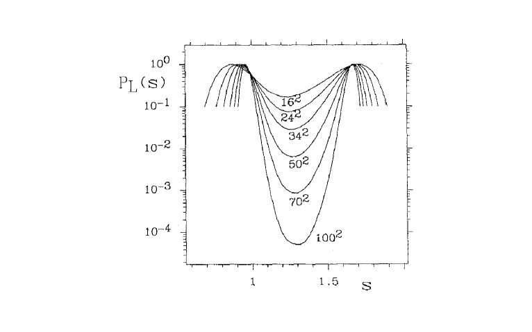
Figure 16: The probability distribution of the energy for different lattice sizes.

$$P_{L}^{(min)}\simeq e^{-\sigma L^{d-1}}\ .$$ (63)

When using a normal Metropolis dynamics eq. (63) implies that the tunneling time diverges severely with the lattice size:

$$\tau_{Metropolis}\simeq AL^{a}e^{\sigma L^{d-1}}\ .$$ (64)

Multicanonical method takes a different approach, by modifying the sampling probability distribution. Here one samples phase space with weight

$$P_{L}^{MCan}\simeq e^{a_{L}^{k}-\beta_{L}^{k}S}\ ,\ \mbox{for}S_{L}^{k}<S\leq S_{L}^{k+1}$$ (65)

(instead of usual $P_{L}^{Bolt}\simeq e^{-\beta_{L}S}$). One has partitioned the action range in intervals $I_{k}$, using a different action in each range. Now one chooses intervals $I_{k}$ and parameters $a_{L}^{k}$, $b_{L}^{k}$ such that $P_{l}^{(MCan)}$ is flat: fig. (17) shows that it can be done very successfully.

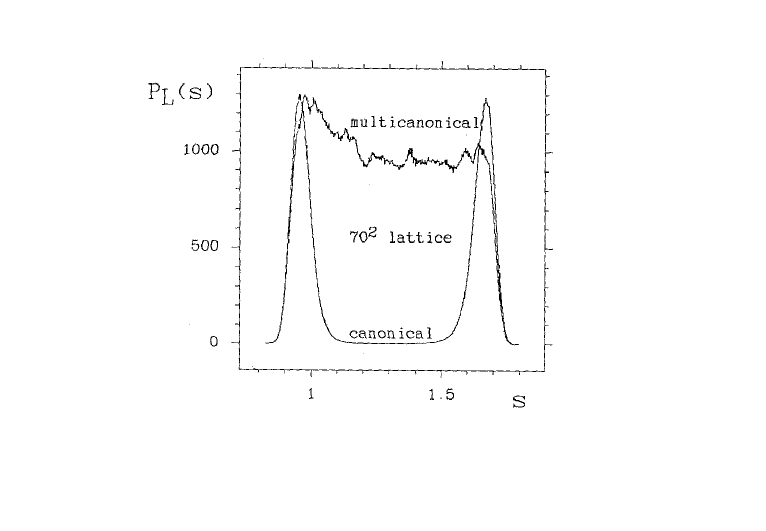
Figure 17: The Boltzmann and the Multicanonical probability distribution of the energy for $L=70$. The multicanonical distribution is quite flat, allowing easy transitions among the two sides of the first order phase transition.

Configurations that were exponentially suppressed are now enhanced by the Multicanonical action: the interested reader can look at details about fixing the parameters in the original papers, [4, 5, 2, 3].

In the case of the Multicanonical algorithm after data collecting you need reweighting (as opposed to tempering, where the output data at each $\beta$ value are directed distributed according to Boltzmann) to reconstruct the Boltzmann distribution. At $\beta^{c}_{L}$

$$P_{L}^{Bolt}=e^{\beta^{c}_{L}S-\beta^{k}_{L}-a_{L}^{k}}P_{L}^{MCan}\ .$$ (66)

The improvement is dramatic, and an exponential slowing down becomes power like ([5]: the same happens for tempering, for example in the cold phase plus to minus tunneling in the Ising model, [12]). An estimate of [5] gives $\tau_{L}^{MCan}\simeq 0.7L^{2.7}$, versus $\tau_{L}^{HeatBath}\simeq 1.5L^{2.15}L^{0.08L}$.

References

- [1]
- [2] Berg B. A., Celik, T. (1992): New Approach to Spin Glass Simulations. Phys. Rev. Lett. 69, 2292.
- [3] Berg B. A., Celik, T., Hansmann, U. (1993): Multicanonical Study of the Ising Spin Glass. Europhys. Lett. 22, 63.
- [4] Berg, B. A., Neuhaus, T. (1991): Multicanonical Algorithms for First-Order Phase Transitions. Phys. Lett. B 267, 249.
- [5] Berg, B. A., Neuhaus, T. (1992): Multicanonical Ensemble: A New Approach to Simulate First-Order Phase Transitions. Phys. Rev. Lett. 68, 9.
- [6] Bhanot, G., et al. (1987). Phys. Rev. Lett. 59, 803.
- [7] Bhatt, R. N., Young, A. P. (1986). J. Magn. Matter 54, 191.
- [8] Caracciolo, S., Pelissetto, A., Sokal, A. D. (1994). Unpublished note.
- [9] Chestnut, D., Salsburg, Z. (1963). J. Chem. Phys. 38, 2861.
- [10] Coluzzi, B. (1995): Heisemberg Spin Glass. J. Phys. A (Math. Gen.)28, 747.
- [11] Falcioni, M., Marinari, E., Paciello, M. L., Parisi, G., Taglienti, B. (1982): Complex Zeroes in the Partition Function of the Lattice Gauge Theory. Phys. Lett. 108B, 331.
- [12] Fernandez, L. A., Marinari, E., Ruiz-Lorenzo, J. (1995): Tempering Dynamics and Relaxation Times in the Ising Model. J. Phys. I (France) 5, 1247.
- [13] Ferrenberg, A., Swendsen, R. (1988): New Monte Carlo Technique for Studying Phase Transitions. Phys. Rev. Lett. 61, 2635.
- [14] Ferrenberg, A., Swendsen, R. (1989): Optimized Monte Carlo Data Analysis. Phys. Rev. Lett. 63, 1195.
- [15] Geyer, J., Thompson, E. A. (1994): University of Minnesota preprint, 1994.
- [16] Graham, J. P., Valleau, J. (1990). Chem. Phys. 94, 7894.
- [17] Hansmann, U. H. E., Okamoto, Y. (1993): Prediction of Peptide Conformation by Multicanonical Algorithm: New Approach to the Multiple-Minima Problem. J. Comp. Chem. 14, 1333.
- [18] Hasenfratz, P. (1996). Contribution to this volume.
- [19] Hukushima, K., Nemoto, K. (1995): Exchange Monte Carlo Method and Application to Spin Glass Simulations. cond-mat/9512035.
- [20] Hukushima, K., Takayama H., Nemoto, K. (1995): Application of an Extended Ensemble Method to Spin Glasses. Int. J. Mod. Phys. C.
- [21] Iori, G., Marinari, E., Parisi, G. (1991). J. Phys. A24, 5349.
- [22] Iori, G., Marinari, E., Parisi, G. (1996). In preparation.
- [23] Itzykson, C., Pearson, R. B., Zuber, J.-B., (1983). Nucl. Phys. B220, 415.
- [24] Kerler, W., Rehberg P. (1994): Simulated Tempering Approcah to Spin Glass Simulations. cond-mat/9402049.
- [25] Kerler, W., Weber, A. (1993): Cluster Dynamics for First-Order Phase Transitions in the Potts Model. Phys. Rev. B47, 11563.
- [26] Kogut, J. (1979): An Introduction to Lattice Gauge Theory and Spin Systems. Rev. Mod. Phys. 51, 659.
- [27] Kondor, I. (1989). J. Phys. A22, L163.
- [28] Kondor, I., Végsö, A. (1993). J. Phys. A26, L641.
- [29] Krauth, W. (1996). Contribution to this volume.
- [30] Marinari, E. (1984): Complex Zeroes of the Ising Model. Nucl. Phys. B235, 123.
- [31] Marinari, E., Parisi, G. (1992): Simulated Tempering: a New Monte Carlo Scheme. Europhys. Lett. 19, 451.
- [32] Marinari, E., Parisi, G., Ritort, F., Ruiz-Lorenzo, J. (1995): Numerical Evidence for Spontaneuosly Broken Replica Symmetry in Spin Glasses. Phys. Rev. Lett. 76, 843.
- [33] Marinari, E., Parisi, G., Ruiz-Lorenzo, J. (1996). In preparation.
- [34] Mc Donald, I., Singer, K. (1967). J. Chem. Phys. 47, 4766.
- [35] Mezard, M., Parisi, G., Virasoro, M. A. (1987): Spin Glass Theory and Beyond. World Scientific, Singapore.
- [36] Montvay, I., Münster, G. (1994): Quantum Fields on a Lattice. Cambridge University Press, Cambridge UK.
- [37] Parisi, G. (1986): A Short Introduction to Numerical Simulations of Lattice Gauge Theories. In Critical Phenomena, Random Systems, Gauge Theories, edited by K. Osterwalder and R. Stora, proceedings of Les Houches, Session XLIII, 1984 (Elsevier, Amsterdam).
- [38] Pearson, R. B. (1982). Phys. Rev. B26, 6285.
- [39] Ritort, F. (1993): Chaos in Short Range Spin Glasses. cond-mat/9307065.
-
[40]
Rose, T., Coddington, P. D., Marinari, E. (1992):
Evaluation of Simulated Tempering for Optimization Problems.
NPAC preprint (Syracuse, NY, USA), unpublished, available at
ftp://ftp.npac.syr.edu/pub/projects/reu/reu92/papers/rose.ps. - [41] Rothe, H. J. (1992): Lattice Gauge Theory: An Introduction. World Scientific, Singapore.
- [42] Salsburg, Z., Jackson, J. D., Fickett, W., Wood, W. W. (1959). J. Chem. Phys. 30, 65.
-
[43]
Shore, M., Coddington, P. D., Fox, G. C., Marinari, E. (1993):
A New Automatic Simulated Annealing-Type Global Optimization Scheme.
NPAC preprint (Syracuse, NY, USA), unpublished, available at
ftp://ftp.npac.syr.edu/pub/projects/reu/reu93/papers/
Shore.ps.Z. - [44] Tesi, M. C.,Janse van Rensburg, E. J., E. Orlandini E., Whillington, S. G. (1995): Monte Carlo Study of the Interacting Self-Avoiding Walk Model in Three Dimensions. Oxford preprint OUTP-95-06S, J. Stat. Phys..
- [45] Torrie, G. M., Valleau, J. P. (1977a). J. Comp. Phys. 23, 187.
- [46] Torrie, G. M., Valleau, J. P. (1977b). Chem. Phys. 66, 1402.
- [47] Valleau, J. P. (1993). In Proceedings of the International Symposium on Ludwig Boltzmann, edited by G. Battimelli, M. G. Ianniello and O. Kreiten.
- [48] Vicari, E. (1993): Monte Carlo Simulation of Lattice Models at Large . Phys. Lett. B309, 139.