The Quantum Toda Lattice Revisited

Abstract

In this work we study the quantum Toda lattice, developing the asymptotic Bethe ansatz method first used by Sutherland. Despite its known limitations we find, on comparing with Gutzwiller’s exact method, that it works well in this particular problem and in fact becomes exact as $\hbar$ grows large. We calculate ground state and excitation energies for finite sized lattices, identify excitations as phonons and solitons on the basis of their quantum numbers, and find their dispersions. These are similar to the classical dispersions for small $\hbar$, and remain similar all the way up to $\hbar=1$, but then deviate substantially as we go further into the quantum regime. On comparing the sound velocities for various $\hbar$ obtained thus with that predicted by conformal theory we conclude that the Bethe ansatz gives the energies per particle accurate to O($1/N^{2}$). On that assumption we can find correlation functions. Thus the Bethe ansatz method can be used to yield much more than the thermodynamic properties which previous authors have calculated.

]

I Introduction

The Toda lattice [3], introduced by M. Toda in 1967 [4], is a chain of particles which interact with nearest neighbours with an exponential potential. The quantum mechanical Hamiltonian for a periodic Toda system of length $N$ (i.e. $n+N\equiv n$) is

$$H=-\sum_{n=1}^{N}\frac{\partial^{2}}{\partial{u_{n}}^{2}}+\eta\sum_{n=1}^{N}e^{-(u_{n+1}-u_{n})}$$ (1)

where the $u_{n}$ are displacements from equilibrium sites. We have chosen appropriate units to remove $\hbar$, $m$ (the mass of the particle) and the length scale of the potential. The infinite system also has a linear term in the potential (to cancel the one in the exponential), but with periodic boundary conditions this vanishes. $\eta$ is a measure of the anharmonicity and also of the scale of the quantum effects. The larger $\eta$ is, the more “classical” the system and the more harmonic the low-energy excitations. In the classical limit the parameter $\eta$ can be scaled out but in the quantum case this can only be done by introducing an $\hbar\neq 1$ in the above equation. We shall occasionally write

$$\hbar=\sqrt{\frac{2}{\eta}}$$ (2)

so that the Hamiltonian can be rescaled and rewritten as

$$\frac{\hbar^{2}}{2}H=-\frac{\hbar^{2}}{2}\sum_{n=1}^{N}\frac{\partial^{2}}{\partial{u_{n}}^{2}}+\sum_{n=1}^{N}e^{-(u_{n+1}-u_{n})}.$$ (3)

The Toda lattice is interesting, classically and quantum mechanically, because it is the one example of a nonlinear lattice which can be solved exactly. Elementary excitations are cnoidal waves, which are periodic waves analogous to the normal modes of a harmonic lattice, and solitons, which are travelling pulse-like solutions which retain their shape even after interaction with other excitations. The periodic system does not support solitons of the infinite-chain type, since these involve a net compression, but a cnoidal wave with large amplitude behaves very much like a soliton (Fig. 1).

The classical periodic system was studied by Kac and van Moerbeke, and Date and Tanaka [5, 6]. It is completely solved [3]: given any initial condition of the system its future time evolution can be written down exactly. In quantum mechanics, there have been several treatments based on various approximations and assumptions. On the one hand, Gutzwiller [7] has given an exact treatment of the 3 and 4 particle lattices, and his quantization algorithm is capable of generalization to larger $N$ as well. His results were rederived in the $r$-matrix formalism by Sklyanin [8] and by Pasquier and Gaudin [9]. The method is plausible and makes a transparent connection with the classical formulation of the problem. On the other hand calculating with this algorithm is a formidable task. The method is summarized in §IV. On the other hand, some authors have used the (asymptotic) Bethe ansatz to treat the problem. Sutherland [10] originally recovered the classical results (high $\eta$) in the thermodynamic limit ($N\rightarrow\infty$). Later authors [11] have remained in this thermodynamic limit, but have looked at arbitrary $\eta$, and have calculated various thermodynamic functions.

In this paper, we use the Bethe ansatz to look at the case of finite $N$, which in some ways is more illuminating when one tries to classify excitations as phonons or solitons. §II obtains the Toda lattice as a limiting case of the $1/\sinh^{2}$ model, an idea due to Sutherland, and §III sets up the Bethe Ansatz equations for the latter model and performs the same limit to obtain equations describing the Toda lattice. Though the asymptotic Bethe ansatz is in general inaccurate for finite $N$, we find in this model that it is much better than it has been given credit for, and in particular becomes exact not only for $N\rightarrow\infty$ but also for $\eta\rightarrow 0$ with finite $N$. In §IV we demonstrate this by setting up exact equations using Gutzwiller’s method and seeing what approximations are involved in going from these to the Bethe equations. The claim [12] that the Bethe ansatz misses a fixed fraction of states does not stand scrutiny. One need only glance at the harmonic limit (§V) where every one of the states is accounted for accurately.

Having done this, we examine the opposite, highly quantum limit in §VI, which makes clearer how the low lying phonon-like modes go over to soliton-like states as their occupation number is increased. §VII calculates dispersion relations for phonons and solitons, and compares the classical and quantum results. We find that the results are essentially the same, apart from the quantization of energy levels, for $\eta>2$ ($\hbar<1$) roughly; but as one decreases $\eta$ further the quantum results deviate more and more from the classical, though they remain qualitatively similar down to $\eta\rightarrow 0$. In this regime we get phonon-like excitations whose energies cannot be derived from harmonic approximations (why we think of them as phonons is discussed in §VII), and soliton-like excitations which can be thought of as authentic examples of the much discussed “quantum soliton”.

§VIII considers finite size effects and makes contact with conformal theory to find correlation functions. We offer evidence that the asymptotic Bethe ansatz, in this problem, gives the energy per particle accurately to order $1/N^{2}$, though on general grounds it is guaranteed only to give results accurate to order 1. Finally, we consider in §IX how all this relates to the classical lattice, and the appendix gives, for completeness, a brief discussion of the other conserved quantities (Hénon’s integrals) and why they are conserved in the classical and quantum cases.

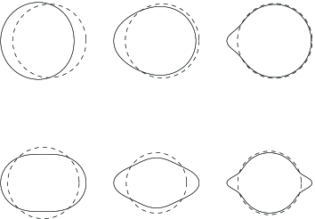
FIG. 1.: How a classical cnoidal wave continuously goes from nearly harmonic to solitonic with increasing amplitude. Above, the first “normal mode” which goes into a one-soliton state. Below, the second mode which goes into a two-soliton state. The same thing happens in our quantum description when we put more and more phonons into a particular phonon mode. (Not to scale)

II Scaling the $1/\sinh^{2}$ model to the Toda model

Sutherland was the first to treat the quantum Toda lattice, as a limiting case of the $1/\sinh^{2}$ model, by pioneering the use of the asymptotic Bethe ansatz. He contented himself with recovering the classical results, and showed that the classical solitons are recovered by taking the classical limit of particle like excitations of the Bethe equations. He did not explore regimes other than the classical, thermodynamic limit. Later authors like Mertens [11] have directly treated the Toda lattice by Bethe’s ansatz, using the phase shifts obtained from the Toda potential; but the validity of the Bethe ansatz (which involves summing over phase shifts a given particle suffers in collisions with all other particles) is unclear in a model where only nearest-neighbour interactions appear. We therefore use Sutherland’s approach and scale the $1/\sinh^{2}$ model. Our scaling procedure is somewhat more explicit and displays the fact that the limiting process leaves us with a one parameter model, the Toda lattice with a general coupling constant $\eta$ ( see below), from which the classical, the harmonic, and the extreme anharmonic limits follow.

Our starting point is the Hamiltonian

$$H_{S}=-\sum_{n=1}^{N}\frac{\partial^{2}}{\partial{x_{n}}^{2}}+g\sum_{{m,n=1}\atop{m<n}}^{N}\frac{1}{\sinh^{2}[(x_{m}-x_{n})/2a]}.$$ (4)

Here $a$ is a length scale giving the range of the potential, $g$ is a coupling constant and the particles are on a ring of length $L$ (so that the density $d=N/L$). In the dilute limit when the particles are far apart, the $\sinh^{2}$ becomes an exponential; we achieve this limit by making the substitution

$$x_{n}=n/d+u_{n}a$$ (5)

where $u_{n}$ are displacements from lattice sites spaced $1/d$ apart. We let $ad$ go to zero, and assume that the $u$’s are bounded (that is, the wavefunction vanishes as $u\rightarrow\infty$). Then we have for $m<n$ and $da\ll 1$,

$$\sinh^{2}\left(\frac{x_{m}-x_{n}}{2a}\right) = \sinh^{2}\left(\frac{m-n}{2ad}+\frac{u_{m}-u_{n}}{2}\right)$$ (6)

$$= (1/4)\exp\left(\frac{n-m}{ad}+u_{n}-u_{m}\right)$$ (7)

and the potential in the Hamiltonian becomes

$$4g\sum_{m<n}\exp\left[-\frac{n-m}{ad}-(u_{n}-u_{m})\right].$$ (8)

So on putting

$$g=\frac{\eta}{4a^{2}}e^{1/ad}$$ (9)

and then allowing $ad$ to go to zero, all terms in the interaction except the nearest-neighbour terms (i.e. $n=m+1$) are killed, and we finally arrive at the Hamiltonian

$\displaystyle a^{2}H_{S}=-\sum_{n=1}^{N}\frac{\partial^{2}}{\partial{u_{n}}^{2}}+\eta\sum_{n=1}^{N}e^{-(u_{n+1}-u_{n})}$

which is the Toda Hamiltonian, eq. (1).

III Solution by the Asymptotic Bethe Ansatz

The $1/\sinh^{2}$ system, being integrable, is characterised by $N$ commuting integrals of motion. If we suppose that the particles are moved far away from one another, they don’t interact except during short-range collisions, and for the rest of the time they have well-defined momenta which can be taken to be the conserved quantities. During two body collisions the most that can happen is an exchange of momenta, and one can show that $n$-particle collisions can be completely described in terms of successive 2-particle collisions and their phase shifts, so that the momenta are reordered but not changed. The Bethe Ansatz is a sum of plane-wave product states, characterized by a set of single-particle momenta {$p_{n}$} and an amplitude for each plane wave state which features a different permutation of these momenta. All that is required for calculation is the two-body phase shift $\theta(p-p^{\prime})$ for two particles with momenta $p$ and $p^{\prime}$ [10]; then equations for the $p_{n}$ can be written down and solved. These equations are

$$p_{n}=\frac{2\pi}{L}I_{n}+\frac{1}{L}\sum_{{m=1}\atop{m\neq n}}^{N}\theta(p_{n}-p_{m}).$$ (10)

Here $I_{n}$ are integers for odd $N$, or half-odd-integers for even $N$, no two of which are equal. The energy (eigenvalue of $H_{S}$) is then given by $\sum{p_{n}}^{2}$, so that the energy of the corresponding Toda problem would be $\sum a^{2}{p_{n}}^{2}$.

This solution is derived in the limit when the particles are far apart, weakly interacting and in approximately plane wave states, so naïvely one would not expect the results to hold at higher densities. It is known, however, that this “asymptotic Bethe ansatz” holds at all densities in the limit $N\rightarrow\infty$ (the thermodynamic limit) provided the virial expansion has no singularities as a function of $d$ [13]. For this particular problem, it turns out that the solution is also exact for arbitrary $N$ in the limit $\eta\rightarrow 0$. Otherwise, though not exact, it is often a very good approximation.

The total momentum is

$$p_{\rm tot}=\frac{2\pi d}{N}\sum_{n=1}^{N}I_{n}.$$ (11)

Owing to the Galilean Invariance of the $1/\sinh^{2}$ model, a state with zero total momentum can always be boosted to have a total momentum $p_{\rm tot}$ by adding an appropriate integer to all the quantum numbers, at a net energy cost $p_{\rm tot}^{2}/N$ independent of the coupling constant. We can take the expression for the two-body phase shift in the $1/\sinh^{2}$ system from Sutherland:

$$\theta(p)=2[\arg\Gamma(1+S+ipa)-\arg\Gamma(1+ipa)]$$ (12)

where $S(S+1)=2ga^{2}=\frac{\eta}{2}e^{1/ad}$. Since we are taking the dilute limit, $S\rightarrow\infty$ for any value of $\eta$, and we can write

$$S=\sqrt{\frac{\eta}{2}}e^{1/2ad}.$$ (13)

In the limit $S\rightarrow\infty$, the phase shift (12) becomes

$$\theta(p)=2pa\log S-2~{}\mbox{Im}~{}\log\Gamma(1+ipa)$$ (14)

[we can show this by using Stirling’s expansion for large $S$ in the first gamma function in (12)]. We substitute for $S$ from (13), put the resulting phase shift into the Bethe equations (10), noting that $\sum_{m}(p_{n}-p_{m})=Np_{n}-p_{\rm tot}$ where $p_{\rm tot}$ is given by (11), and rearrange [the $p_{n}$ on the left of (10) cancels with a term from the phase shift, leaving only O($1/L$) and smaller terms]. Defining dimensionless “momenta” by $k_{n}=p_{n}a$, dividing out the common $d$ and taking $ad\rightarrow 0$ we end up with the equations to be solved:

$$\alpha k_{n} = -\frac{\pi}{N}\left(I_{n}-\frac{\Sigma I_{n}}{N}\right)$$ (16)

$$+\frac{1}{N}\sum_{{m=1}\atop{m\neq n}}^{N}~{}\mbox{Im}~{}\log\Gamma[1+i(k_{n}-k_{m})]$$

where for convenience we have written

$$\alpha=\frac{1}{2}\log\left(\frac{\eta}{2}\right)(=-\log\hbar).$$ (17)

Note that the total momentum of the system, $k_{\rm tot}=(ad)(2\pi/N)\sum_{j}I_{j}$, goes to zero as $ad$ goes to zero, so that we are working in a zero momentum frame. This is a consequence of the length of the underlying $1/\sinh^{2}$ model going to infinity (on the scale of the range of the potential), the momentum being inversely proportional to the system length. However, our simultaneous scaling up of the interaction by an exponential factor (9) ensures that the individual particle momenta remain finite. Thus we have gone from a $1/\sinh^{2}$ “gas” with particles described by actual position coordinates, to a lattice with particle positions described as displacements from lattice sites, and no net momentum, which is what we wanted. The energy of this Toda problem is $\sum k^{2}_{n}$. Since the problem continues to be Galilean invariant, a finite momentum $k_{\rm tot}$ can always be introduced into the above equations by adding $\alpha k_{\rm tot}/N$ to the right hand side, at a total energy cost of $k^{2}_{\rm tot}/N$. This $k_{\rm tot}$ need not be quantized, since as the length of the underlying $1/\sinh^{2}$ model expands the quanta of momentum become infinitesimal.

The $I_{n}$ in (10) and (16) are the quantum numbers of the system, and uniquely specify the state of the system. The momenta $k_{n}$ are ordered in the same way as $I_{n}$ [despite the apparently opposite sign for $\eta>2$ in (16)] and we assume that the order is ascending in $n$. In the ground state the $I_{n}$ are successive integers (or half integers), generally taken to be centred about zero [though it does not matter here, since one subtracts their average value in Eq. (16)] and in the excited states one or more of them are increased by various integer values, always making sure no two of them have the same value.

Although we took the dilute limit in arriving at these equations, the Toda Hamiltonian (1) which they describe contains no reference to the lattice constant, and therefore they are valid at all densities, or at least at all densities sufficiently low that the particles do not cross each other. (The wavefunction will give the typical “spread” in $u_{n}$ and we must assume, for physical reasons, that the inter-particle separation is much larger than this). Mertens’ treatment [11], if followed through, gives the same equations as the above but with an extra term on the right hand side equal to $(2\pi ad/N)\sum I_{n}$ (which is the above $k_{\rm tot}$: he does not consider a limiting case of the $1/\sinh^{2}$ model and does not take $d\rightarrow 0$). This term has no significance and, in particular, must not be confused with the phonon or soliton momenta (§VII). In fact, it may be subtracted out, since it is independent of $n$, to recover our equations. We prefer this, the rest frame, because it is the frame in which one normally discusses phonons and also because it is convenient in making contact with Gutzwiller’s work.

Since one can add a constant quantity to the $I_{n}$ without effect on the equations, they contain some redundancy—$N-1$ quantum numbers are enough to characterize the system. We could define new quantum numbers by

$$\nu_{n}=I_{N-n+1}-I_{N-n}-1,~{}~{}~{}n=1,2,\ldots,N-1$$ (18)

so that the $\nu_{n}$ may take any integer value from 0 upwards. (These are the number of “holes” between successive integers $I_{n}$, starting from the right.) These are, in the harmonic limit, the phonon occupation numbers (§V).

Equations (16) can be solved numerically, for instance by the Newton-Raphson method, for moderate values of $N$ without much difficulty if one has a good starting guess. If not, the numerical methods tend to converge to spurious solutions where the ordering of the $k$’s is not the same as that of the $I$’s.

Alternatively, one could pass to the thermodynamic limit and write down integral equations from which various thermodynamic quantities could be calculated, as in Yang and Yang’s treatment of the $\delta$-function Bose gas. This has been done by Mertens, and by Hader and Mertens [11]. We define $(N/2\pi)\xi(k)dk$ as the number of $k$’s between $k$ and $k+dk$. Then (16) yields the integral equation for the density of the $k$’s in the ground state which is, in agreement with Mertens,

$$\xi(k)=-2\alpha+\frac{1}{\pi}\int_{-B}^{B}\xi(k^{\prime})~{}\mbox{Re}~{}\psi(1+i(k-k^{\prime}))dk^{\prime}.$$ (19)

($\psi$ is the digamma function). For reasons given in the next section, Matsuyama [14] gets the same equation for the distribution of the zeros of Hill’s determinant in the Gutzwiller method (but without the inhomogeneous part since he takes $\hbar=1$, or $\eta=2$.)

IV Comparison with Gutzwiller’s formulation

The Bethe equations for the Toda lattice can also be derived from Gutzwiller’s solution of the problem, if some approximations are made. This helps clarify what the $k$’s mean in the non-dilute limit—in particular, their correspondence with the classical variables, and also tells us when our approximations are valid. We briefly describe Gutzwiller’s method and the resulting quantization conditions.

Gutzwiller, following the classical ideas of Kac and van Moerbeke [5], tries to write the wavefunction of the $N$ body lattice as a series involving the wavefunctions of the $N-1$ body open lattice obtained by removing one particle. Suppose these $N-1$ body wavefunctions are $\Psi_{\kappa_{1}\kappa_{2}\ldots\kappa_{N-1}}$; the indices $\kappa$ correspond to the classical variables $\mu_{i}$ (the eigenvalues of the truncated $N-1$ dimensional Lax matrix). For the open chain they are purely imaginary but when using them as a basis in the closed chain Gutzwiller shows that one must extend them to have a real integer part; in other words, $\kappa_{i}=i\rho_{i}+k_{i}$, where $k_{i}$ is an integer. One aims to find the spectrum of the $\rho$’s. It turns out that if one writes the wavefunction as $\Psi=\sum C_{\kappa_{1}\kappa_{2}\ldots\kappa_{N-1}}\Psi_{\kappa_{1}\kappa_{2}\ldots\kappa_{N-1}}$, where the sum is over the integers $k_{i}$, one can get a solution of the form $C_{\kappa_{1}\kappa_{2}\ldots\kappa_{N-1}}=(\kappa_{1}-\kappa_{2})(\kappa_{2}-\kappa_{3})\ldots r_{\kappa_{1}}s_{\kappa_{2}}t_{\kappa_{3}}\ldots$ provided the coefficients $r$, $s$, $\ldots$ satisfy identical recursion relations

$$i^{N}r_{\kappa+1}+i^{-N}r_{\kappa-1}=D(\kappa)r_{\kappa}$$ (20)

where $D(\kappa)$ is basically the characteristic polynomial of the Lax matrix (see the appendix):

$$D(\kappa) = \hbar^{N}\kappa^{N}+E\hbar^{N-2}\kappa^{N-2}+iA_{3}\hbar^{N-3}\kappa^{N-3}+$$ (22)

$$\ldots+(-i)^{N-1}A_{N-1}\hbar\kappa+(-i)^{N}A_{N},$$

and $\hbar$ is defined in (2). Suppose that its zeroes are $i\epsilon_{1},i\epsilon_{2},\ldots,i\epsilon_{N}$; then $D(\kappa)$ can also be written as

$$D(\kappa)=\prod_{n}(\hbar\kappa-i\epsilon_{n}).$$ (23)

The same recursion relations are derived by Sklyanin, and by Pasquier and Gaudin, from different points of view [8, 9]. They have two independent solutions, differing in their behaviour at $+\infty$ and $-\infty$. Gutzwiller sets

$$r_{\kappa}^{(1)}=\frac{(-1)^{\kappa}r^{\prime}}{\hbar^{N\kappa}\prod_{i}\Gamma(1+\kappa-i\epsilon_{i})}r^{\prime}_{\kappa},$$ (24)

$$r_{\kappa}^{(2)}=\frac{(-1)^{\kappa}r^{\prime\prime}}{\hbar^{-N\kappa}\prod_{i}\Gamma(1-\kappa+i\epsilon_{i})}r^{\prime\prime}_{\kappa},$$ (25)

where $r^{\prime}$ and $r^{\prime\prime}$ are coefficients to be matched later when “joining” the two solutions, and $r^{\prime}_{\kappa}$ and $r^{\prime\prime}_{\kappa}$ are two new variables which (it turns out) are complex conjugate. They have solutions

$$r^{\prime}_{\kappa}=\left|\begin{array}[]{cccc}1&\frac{\pm 1}{D(\kappa+1)}&&0\\[5.0pt] \frac{1}{D(\kappa+2)}&1&\frac{\pm 1}{D(\kappa+2)}&\\[5.0pt] &\frac{1}{D(\kappa+3)}&1&\\[5.0pt] 0&&&\ddots\end{array}\right|,$$ (30)

$$r^{\prime\prime}_{\kappa}=\left|\begin{array}[]{cccc}\ddots&&&0\\[5.0pt] &1&\frac{\pm 1}{D(\kappa-3)}&\\[5.0pt] &\frac{1}{D(\kappa-2)}&1&\frac{\pm 1}{D(\kappa-2)}\\[5.0pt] 0&&\frac{1}{D(\kappa-1)}&1\end{array}\right|.$$ (35)

The former approaches a constant as $k\rightarrow+\infty$, and the latter approaches a constant as $k\rightarrow-\infty$.

If one tries to join these solutions, one gets the consistency condition

$$\Delta(\kappa)=\left|\begin{array}[]{ccccc}\ddots&\frac{\pm 1}{D(\kappa-2}&&&0\\[5.0pt] &1&\frac{\pm 1}{D(\kappa-1)}&&\\[5.0pt] &\frac{1}{D(\kappa)}&1&\frac{\pm 1}{D(\kappa)}&\\[5.0pt] &&\frac{1}{D(\kappa+1)}&1&\\[5.0pt] &&&\frac{1}{D(\kappa+2)}&\\[5.0pt] 0&&&&\ddots\end{array}\right|=0.$$ (36)

Here the $+$ signs are for even $N$, the $-$ signs for odd $N$. This determinant has $N$ purely imaginary zeroes, which we call $i\rho_{1},i\rho_{2},\ldots,i\rho_{N}$ (in ascending order). (If $N$ is odd and all odd integrals $A_{3},A_{5},\ldots$ vanish—this happens, for instance, in the ground state—then there are only $N-1$ zeroes but in that case $\kappa=0$ also satisfies the quantization conditions below, so we include it among the $\rho$’s.) It is clear that in addition to these, $i\rho_{n}+l$, where $l$ is an arbitrary integer, are also zeroes of the determinant.

The determinant is part of what we need to find the spectrum of $\rho$, but it is not enough since we don’t know the constants of motion in $D(\kappa)$. We need more quantization conditions; to supply these Gutzwiller defines an angle $\phi=(1/2)\arg(r^{\prime}/r^{\prime\prime})=\arg(r^{\prime})$ since $r^{\prime}$ and $r^{\prime\prime}$ are complex conjugate. If one normalizes the solutions by $r_{i\rho}^{(1)}=r_{i\rho}^{(2)}=1$, one finds

$$\phi=\arg(r^{\prime})=~{}\mbox{Im}~{}\log\left(\frac{\hbar^{iN\rho}\prod_{m}\Gamma(1+i[\rho-\epsilon_{m}])}{{r^{\prime}_{i\rho}}}\right).$$ (37)

Then $\phi$ is a monotonically increasing function of $\rho$. Abbreviating $\phi(\rho_{n})$ as $\phi_{n}$, Gutzwiller’s quantization condition reads

$$\phi_{1}=\phi_{2}=\ldots=\phi_{N}~{}~{}~{}~{}(\mbox{modulo}~{}~{}\pi).$$ (38)

In addition he assumes that

$$\phi_{1}+\phi_{2}+\ldots+\phi_{N}=0.$$ (39)

If both of these conditions are satisfied, the allowed values of $\phi_{n}$ are very limited; they can only be of the form $I_{n}\pi+m\pi/N$, where $m$ is the same integer for all $n$ and $I_{n}$ is an arbitrary integer, different for different $n$. But $\phi_{n}$ is an increasing function of $\rho_{n}$, hence if the $\rho_{n}$ are ordered, we must have the $I_{n}$ also in increasing order. Then, from (39), we get

$$\sum_{n}\pi I_{n}+m\pi=0$$ (40)

which yields $m=-\sum I_{n}$. So we have, finally, expressions for Gutzwiller’s phase angles:

$$\phi_{n} = \pi\left(I_{n}-\frac{\sum I_{m}}{N}\right)$$ (41)

$$= \arg r^{\prime}=\arg\left(\frac{\hbar^{iN\rho_{n}}\prod_{m}\Gamma(1+i[\rho_{n}-\epsilon_{m}])}{r^{\prime}_{i\rho_{n}}}\right)$$ (42)

$$= -\alpha N\rho_{n}+\sum_{m}~{}\mbox{Im}~{}\log\Gamma(1+i[\rho_{n}-\epsilon_{m}])$$ (44)

$$-~{}\mbox{Im}~{}\log r^{\prime}_{i\rho_{n}},$$

or

$$\alpha\rho_{n} = -\frac{\pi}{N}\left(I_{n}-\frac{\sum I_{m}}{N}\right)$$ (47)

$$+\frac{1}{N}\sum_{m}~{}\mbox{Im}~{}\log\Gamma(1+i[\rho_{n}-\epsilon_{m}])$$

$$-\frac{~{}\mbox{Im}~{}\log r^{\prime}_{i\rho_{n}}}{N}.$$

($\alpha=\mbox{$\frac{1}{2}$}\log(\eta/2)=-\log\hbar$.) These, then, are the exact Gutzwiller equations which can be combined with (36) to calculate the $\rho_{n}$ and $\epsilon_{n}$; once the latter are known, all the conserved quantities can be found. The $I_{n}$ in this equation are the quantum numbers of the system, and are the same as the $I_{n}$ in the earlier, very similar Bethe ansatz equations (16)— to which these equations in fact reduce provided (1) the last term can be ignored and (2) $\rho_{n}$ is very close to $\epsilon_{n}$ for all $n$. These things can happen under two circumstances.

There is an argument in [14] showing that the $\rho_{n}$ should approach $\epsilon_{n}$ as $N\rightarrow\infty$ (and one knows on general grounds that the asymptotic Bethe ansatz is correct in this limit). This also happens as $\hbar\rightarrow\infty$, for finite $N$. We can understand the latter fact intuitively as follows: As $\hbar\rightarrow\infty$, the polynomials $D(\kappa)$ tend to infinity. (This is not obvious—for example, they don’t vanish as $\hbar\rightarrow 0$ —but it will be demonstrated in §VI). Then they will be small only in a small region close to their zeroes, so the matrix of which (36) is the determinant tends to the unit matrix except when $\rho_{n}$ lie in some small regions surrounding $\epsilon_{n}$. Thus the determinant can only vanish when the $\rho$’s approach the $\epsilon$’s; otherwise it is close to unity. For the same reason, (30) tends to unity (its zeroes will be close to $i\rho_{n}+l=0$, $l\geq 1$, and for $\kappa=i\epsilon_{n}$ all the $D$’s in the denominators will be very large). Then the last term in (47) will vanish, and all the $\rho$’s can be substituted with $\epsilon$’s, and we recover exactly the Bethe ansatz equations.

Thus the Bethe ansatz is actually more accurate in the quantum limit than in the classical limit. Indeed, even for $\hbar=1$ and $N$ = 4–6, the agreement with Matsuyama’s exact diagonalization results [15] is excellent (one gets exactly his answers, to his reported accuracy) —and this looks neither like a thermodynamic limit nor like an extreme quantum limit.

One might imagine that the Bethe ansatz equations could be improved by subtracting the term $\frac{1}{N}~{}\mbox{Im}~{}\log r^{\prime}_{ik_{n}}$, but it turns out that this term is always small compared to the others and does not greatly improve the results, while it is computationally expensive to include; therefore we ignore it in all cases.

Finally, we observe that equations (47) do not remain the same if the $\rho$’s and $\epsilon$’s are increased by a constant quantity, because of the last term which does not appear in the Bethe ansatz equations. We cannot therefore transform these easily to a non-zero-momentum frame.

V The harmonic limit (high $\eta$)

For large $\eta$ (the classical limit) the lattice is harmonic, at least for sufficiently small quantum numbers. The larger $\eta$ is, the larger the energies and the quantum numbers required for anharmonicity to show up. Treating this case makes clear the mapping between the phononic quantum numbers and the $I_{n}$.

First, the exact solution. There are $N-1$ normal modes in the system, characterized by “phonon momenta” or wavenumbers $q_{n}=2\pi n/N$, where $n$ = 1 …$N-1$. In our notation the coefficient of the $u^{2}$ terms in (1) is $\eta/2$. Then the frequency $\omega_{n}$ of the $n$th mode is

$$\omega_{n}=2\sqrt{2\eta}\sin\left(\frac{q_{n}}{2}\right).$$ (48)

An arbitrary state of the system is then characterised by a set of nonnegative integers { $\nu_{n}$ } (phonon occupation numbers). The energy of such a state is

$$E = N\eta+\sum_{n=1}^{N-1}(\nu_{n}+\mbox{$\frac{1}{2}$})\omega_{n}$$ (49)

$$= N\eta+2\sqrt{2\eta}~{}\sum_{n=1}^{N-1}(\nu_{n}+\mbox{$\frac{1}{2}$})\sin\left(\frac{\pi n}{N}\right).$$ (50)

The first term arises from the constant term in the Taylor expansion of the exponential potential. For the ground state, we set $\nu_{n}=0$ and find

$$E=N\eta+\sqrt{2\eta}\;\cot(\frac{\pi}{2N})$$ (51)

which for large $N$ has an expansion

$$E=N\eta+\sqrt{2\eta}\;[\;\;\frac{2}{\pi}N-\frac{\pi}{6N}+O(1/N^{3})].$$ (52)

Now we compare this expression with the result of solving Eqs (16) numerically for 10 particles, and for various “large” $\eta$ : 10, 100, and higher. The ground state is when the $I_{n}$ are contiguous, with no “holes”; the energy calculated from (49) is in good agreement with the value obtained from the Bethe ansatz. Numerical calculations show that the $\nu_{n}$ which describe a phononic state are exactly the numbers defined in (18). In other words, the number of phonons in a mode $n$ is given by the number of holes between $I_{N-n}$ and $I_{N-n+1}$.

This prescription accounts for all the states of the harmonic lattice, and the quantitative agreement is very close for low phonon numbers (the higher $\eta$ is, the higher the allowed phonon numbers before anharmonic effects start showing up). Fig. 2 gives the dispersion curve for single phonons; only for low $\eta$ does it differ from the harmonic-lattice curve. Calculations show that the energies of phonons are additive (provided there are not too many of them) so multi-phonon states are also accurately described.

VI The strongly-quantum anharmonic limit ($\eta\rightarrow 0$)

In the large-$\eta$ case, increasing occupation numbers will bring out anharmonic corrections in the energy, and modes with very high occupation numbers will resemble solitons. In §VII we demonstrate this with calculations, but if $\eta$ is not large anharmonicity shows up even in low-lying modes.

Having looked at the harmonic limit in the last section, we now look at the opposite limit of the lattice, $\eta\rightarrow 0$; in this case it turns out that the phase shift simplifies greatly, and we can in fact solve equations (16) for $k_{n}$—an uncommon phenomenon in Bethe ansatz calculations.

Equation (14) for the phase shift is

$\displaystyle\theta(k)=2k\log S-2~{}\mbox{Im}~{}\log\Gamma(1+ik),$

and as $\eta\rightarrow 0$, $k$ also becomes small. In this limit the term involving the gamma function becomes $2\gamma k$, where $\gamma=0.577215...$ is Euler’s constant. A quick way to derive this result is to assume $S$ is a large integer in (12) and to expand the first gamma function as a product $(S+ik)(S-1+ik)\ldots(1+ik)\Gamma(1+ik)$, and if $k\ll 1$, the argument of this is $k/S+k/(S-1)+\ldots+k$ + a piece which cancels the second term in (12). As $S\rightarrow\infty$, using the definition $\gamma=\lim_{n\rightarrow\infty}1+(1/2)+(1/3)+\ldots+(1/n)-\log n$, the phase shift becomes

$$\theta(k)=2k(\log S+\gamma)$$ (53)

(this is actually correct to quadratic order in $k$), which when substituted in (10) yields

$$k_{n} = \frac{2\pi d}{N}I_{n}+\frac{2d}{N}(\gamma+\log S)\sum_{m\neq n}(k_{n}-k_{m})$$ (54)

$$= \frac{2\pi d}{N}I_{n}+\frac{2d}{N}(\gamma+\log S)(Nk_{n}-k_{\rm tot})$$ (55)

and on substituting for $k_{\rm tot}$ from (11) and rearranging, we find

$$k_{n}=-\frac{\pi\left(I_{n}-\frac{\Sigma I_{n}}{N}\right)}{N(\gamma+\alpha)}.$$ (56)

(Note that for very small $\eta$, $\alpha$ will be large and negative, so the negative sign above is deceptive; the $k$’s are ordered in the same way as the $I$’s.) Equations (56) thus give $k_{n}$ for any excited state specified by any integers $I_{n}$, and the energy is $\sum k_{n}^{2}$ as before. Note that the system now looks like a free Fermi gas or a hard-sphere gas, which indeed is the underlying model behind the asymptotic Bethe ansatz (we derived our results as a limiting case of a gas of particles interacting by a $1/\sinh^{2}$ potential). There is a continuous transition from this system to the classical Toda lattice as $\eta$ is increased. As we show below, even in this limit the excitations retain their qualitative features.

In the ground state, the $I_{n}$ are contiguous and may be taken to be 1, 2, …, $N$. Then a simple calculation gives the ground state energy as

$$E_{0}=AN(N^{2}-1)/12\approx AN^{3}/12$$ (57)

where

$$A=\frac{\pi^{2}}{N^{2}(\alpha+\gamma)^{2}}.$$ (58)

Now we consider excitations in which the last $l$ $I_{n}$ are excited by an amount $m$—we insert $m$ holes between $I_{N-l}$ and $I_{N-l+1}$, or in the phonon language, we add $m$ phonons in the $l$th normal mode. $I_{n}$ are now 1, 2, 3, …, $N-l$, $N-l+m+1$, $N-l+m+2$, …, $N+m+1$. Again, one can calculate the excitation energy; it is

$$E-E_{0}=A(Nl-l^{2})\left(m+\frac{m^{2}}{N}\right).$$ (59)

We consider several cases:

1. $m$ small, arbitrary $l$

   In this case, we get approximately

   $$E-E_{0}=A(Nl-l^{2})m.$$ (60)

   This looks very much like a phonon dispersion; it rises from zero to a maximum at the zone boundary, where its slope dies off. It is linear in the number of “quanta” $m$, and for the lower-energy modes (lower $l$) it is also linear in mode number or wavenumber (i.e. the 2nd mode has twice the energy of the first mode, and so on).

   Moreover, for phonons we know that the zero point energy in each mode is half the energy of one phonon; we can therefore sum half the above expression over $l$, for $m=1$, and see, as a check, whether we recover the zero point energy (57). And indeed, we do get

   
   

   $\displaystyle\sum_{l-1}^{N-1}\mbox{$\frac{1}{2}$}A(Nl-l^{2})=\mbox{$\frac{1}{12}$}AN(N^{2}-1)$

   in agreement with (57).

   The excitations are non-interacting—if we have several such excitations in different modes their combined energy is the sum of their individual energies, if there are not too many of them. These hole excitations are thus quite analogous to phonons, though they cannot be derived by approximating the lattice to a harmonic lattice.

2. $l=1$, $m$ large

   These are the excitations which one would expect to be soliton-like. In this limit, we get

   $$E-E_{0}=A(N-1)\left(m+\frac{m^{2}}{N}\right)$$ (61)

   For large $m$ the energy is thus quadratic in $m$. This energy, however, is measured in the zero-momentum frame which is not the frame in which one normally discusses solitons. The question of what is the correct frame is discussed in the next section, where dispersion relations are derived.

3. $l$ small, $m$ large

   From (59) we note that if $l$ is small, the excitation energy is proportional to $l$. For instance, the energy for $l=2$ is twice that for $l=1$. It is tempting to suppose that this is a two soliton state, since the energies of solitons are additive provided that they are few in number and hence well separated “most of the time”. In that case there would be a continuous transition between a phononic excitation of the second normal mode and the two soliton state, just as there is between the excitation of the first normal mode and the one soliton state. (Cf. Fig. 1, and §IX)

If the last two integers are excited by different amounts, one would presumably have two solitons with different energies. Here, too, the total excitation energy is the sum of the individual energies. Carrying this picture further, an $N-1$ soliton state (with all solitons having equal energies—$l=N-1$, $m$ large) has all the particles except one moving in one direction like hard spheres, and is related by a Galilean transformation to a 1 soliton state. An $N$ soliton state (with all solitons identical) is simply a uniform translation of the lattice as a whole. One cannot put more than $N$ solitons in an $N$-particle lattice. The last few sentences are speculative, but they indicate the possibility of writing an arbitrary excited state as a kind of nonlinear superposition of solitons. (To make this more convincing, read cnoidal waves for solitons). Much the same thing is done in the classical periodic system (§IX).

VII Dispersion relations for phonons and solitons

We now find the dispersion relations for phonons and solitons. First, however, we clarify the meaning of the momentum of these excitations.

As remarked earlier, the fact that we take the dilute limit gives us a zero total momentum. Mertens’ treatment, on the other hand, yields a finite momentum $\sum k_{n}$ proportional to $\sum I_{n}$ and to the density $d$. This momentum is not a physically relevant quantity. It is not the momentum of a phonon (though it is proportional to it), since it depends on $\eta$ while the phonon momentum is a purely geometrical quantity depending only on the system size and lattice spacing. Nor is it the momentum of a soliton (it is not even proportional) since the soliton momentum doesn’t depend on the lattice spacing.

The phonon momentum $q$ is the wavenumber of an oscillatory excitation. For an $N$ particle lattice $q$ has $N$ equally spaced values generally taken to lie between $-\pi$ and $\pi$ (the first Brillouin zone) in units of the inverse lattice spacing. The soliton momentum is a little trickier to define in the quantum case. We discuss it below.

First consider the small $\eta$ limit. We consider a single phonon, occupying normal mode $n$; its excitation energy, from (60) with $l=n$ and $m=1$, is $E-E_{0}=A(Nn-n^{2})$ and its wavenumber $q$, in units of inverse lattice spacing, is $2\pi n/N$ (modulo $2\pi$; we can choose the value to lie between $-\pi$ and $\pi$.) Note that $\sum I_{m}=n$ in this case, if it was taken to be zero in the ground state, so $q$ is proportional to this quantity. This gives $\omega$, the frequency (or the excitation energy of one phonon, since $\hbar=1$) in terms of $q$ as

$$\omega=\frac{\pi}{2(\gamma+\alpha)^{2}}\left[q-\frac{q^{2}}{2\pi}\right],~{}~{}~{}~{}0<q<2\pi$$ (62)

and the phase velocity of sound is

$$v_{\mbox{p}}=\frac{\pi}{2(\gamma+\alpha)^{2}}\left[1-\frac{q}{2\pi}\right]$$ (63)

while the group velocity is

$$v_{\mbox{g}}=\frac{\pi}{2(\gamma+\alpha)^{2}}\left[1-\frac{q}{\pi}\right].$$ (64)

(in units of the lattice spacing).

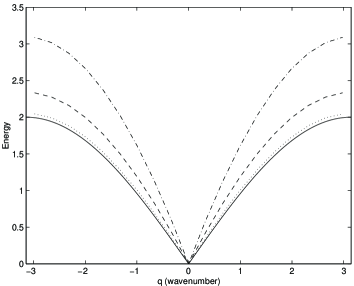
FIG. 2.: Phonon energies (for the Hamiltonian (3, in units of $\hbar$), plotted against wavenumber $q$ for various $\eta$. The solid line is the harmonic lattice curve and the curves for all “large” values of $\eta$ lie on top of it. The dotted line is for $\eta=2$, the dashed line $\eta=0.1$, the dotdash line $\eta=0.01$. The range of $q$ is [$-\pi$,$\pi$]. Energies are in units of $\sqrt{2\eta}$ (using the Hamiltonian (1); or with the Hamiltonian (3) energies are in units of $\hbar$). Here and in later graphs, units are chosen to get an $\eta$-independent curve in the large $\eta$ limit.

In the classical limit, of course, the phonons are what one would find from a harmonic approximation. For a mode with wavenumber $q$ the energy is

$$E-E_{0}=2\sqrt{2\eta}\sin\mbox{$\frac{1}{2}$}q$$ (65)

which yields the phase velocity (in units of lattice spacing)

$$v_{\mbox{p}}=2\sqrt{2\eta}\frac{\sin\mbox{$\frac{1}{2}$}q}{q}$$ (66)

and the group velocity

$$v_{\mbox{g}}=\sqrt{2\eta}\cos\mbox{$\frac{1}{2}$}q.$$ (67)

The relations are different in the two cases, but have some similar features, and at intermediate values of $\eta$ one obtains interpolations between these. Dividing the energies of excitation by $\sqrt{2\eta}$ one gets results independent of $\eta$ in the classical limit $\hbar\rightarrow 0$ or $\eta\rightarrow\infty$. The results are plotted in Figs. 2 and 3 (for a nineteen particle lattice). One observes that for $\eta>2$ the dispersion is more or less the classical harmonic-lattice dispersion, while it begins to deviate for $\eta<2$. This is further emphasized by Fig. 4 which shows how the long wavelength sound velocity varies with $\alpha=-\log\eta$.

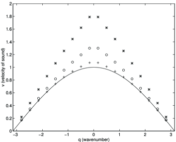
FIG. 3.: The velocity of sound, $dE/dq$, plotted against $q$ for various $\eta$ for a 19 particle lattice. The solid line is the curve for the harmonic lattice, valid for large $\eta$. The crosses represent $\eta=2$, the circles $\eta=0.1$, the asterisks $\eta=0.01$. Units are as in the previous graph for the phonon dispersion.

When we consider a soliton, we have to make clear what frame to view it in to obtain an appropriate momentum. In the classical case it is usually viewed in the frame where “most” of the particles are at rest and only a localized excitation is moving. We would like to choose a frame in the quantum case such that the dispersion agrees with the classical formula; in particular as the energy of the excitation increases it behaves more and more like a single hard sphere moving in a stationary background and the energy tends to $k^{2}$ (plus the ground state energy).

We identify a soliton with a state where $k_{N}$ is greatly excited compared to all the other $k$’s. We can achieve the $k^{2}$ dispersion if we work in a frame where the $k$’s excluding $k_{N}$ are (roughly speaking) centred around zero. In that case for large excitations $k_{N}\gg k_{n}$ ($n<N$), the total momentum is very nearly $k_{N}$, the total energy is nearly ${k_{N}}^{2}\approx k^{2}$, and the quadratic dispersion is achieved.

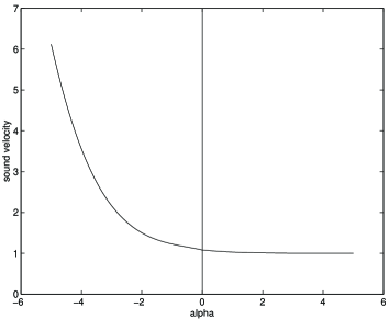
FIG. 4.: Variation of long-wavelength sound velocity, in the same units as in Figure 3, as a function of $\alpha$ ($=-\log\hbar$ = $(1/2)\log(\eta/2)$). Note that $\alpha=0$ seems to divide the harmonic and quantum anharmonic regimes, i.e. the region where the harmonic approximation is valid for small excitations and the region where the zero point motion is so large that the harmonic approximation is not valid even in the ground state.

However, exactly how to define the frame is not clear. There are various possibilities—one could choose the average of all $k_{n}$ except $k_{1}$ and $k_{N}$ to be zero (so that the $k$’s are not very much displaced from the ground state value); one could make the average of $k_{n}$ including $k_{1}$ but excepting $k_{N}$ zero; one could fix one of the $k$’s (say $k_{1}$, $k_{N/2}$ or $k_{N-1}$) to its ground state value; and so on. These possibilities are plotted in Fig. 5, for $\eta=1000$, and the dispersion for a classical cnoidal wave of wavelength $N$ plotted for comparison, calculated from the formula for $r_{n}=u_{n}-u_{n-1}$ given in [3] (cf. §IX). Of the possibilities listed the second (where the $k$’s excepting $k_{N}$ average to zero) seems the closest to the classical curve, but the agreement is imperfect and the “correct” frame would appear to be something close but slightly different. In plotting these curves we have used the Hamiltonian (3), whose limit as $\hbar\rightarrow 0$ is the classical problem in the correct units. Fig. 5 shows the dispersion curves for $\eta=1000$.

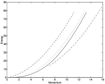
FIG. 5.: Dispersion curves for the classical and quantum cnoidal waves. The solid curve is the classical cnoidal wave or soliton, viewed in the appropriate frame. The dotted curve is the quantum cnoidal wave in a frame in which $\sum_{n=1}^{N-1}k_{n}=0$. This lies closest to the classical curve among the cases considered. The dashed curve corresponds to the frame in which only the “inner” $k$’s are centred at zero, i.e. $\sum_{n=2}^{N-1}k_{n}=0$ (as in the ground state of the system). The dotdash curve corresponds to $k_{N}-1$ being fixed at its ground state value—implausible perhaps but included here for variety. All curves are for $N=10$ and (in the quantum case) for $\eta=1000$. The Hamiltonian (3) is used; in other words energies from the Hamiltonian (1) are plotted in units of $\eta$.

Fig. 6 shows the particular dispersion curve obtained by averaging $k_{n<N}$ to zero, for various $\eta$. As in the case of the phonon curves, the soliton dispersions lie on top of each other for large $\eta$ but begin peeling apart for $\eta\approx 2$; as $\eta$ is reduced further they move further and further away. Thus we find again that $\eta=2$ or $\hbar=1$ is a boundary between classical and quantum regimes. For higher $\eta$ the dispersions are essentially the classical ones apart from the discreteness of the energy levels. For lower $\eta$ the results deviate significantly from the classical ones. All the curves above have been calculated for a ten particle lattice.

In the $\eta\rightarrow 0$ limit we have the $k_{n}$ given by (56); for the ground state state we take the $I_{n}$ to be centred at zero (i.e. they range from $-(N-1)/2$ to $(N-1)/2$ for odd $N$, or from $-N/2$ to $N/2$ for even $N$); and for the soliton we excite $I_{N}$ by an amount $m$. Then $\sum I_{n}=m$. Clearly if we want the $k_{n}$ (for $n<N$) to be centred at zero, we must add to (56) a quantity to cancel the $\sum I_{n}/N$ in the numerator, and instead subtract $\sum_{n=1}^{N-1}I_{n}/(N-1)$. In this new frame, we have

$$k_{n} = -\frac{\pi\left(I_{n}-\frac{\sum_{m=1}^{N-1}I_{m}}{N-1}\right)}{N(\gamma+\alpha)},$$ (68)

$$k = \sum k_{n}=-\frac{\pi(m+N/2)}{N(\gamma+\alpha)},$$ (69)

$$E-E_{0} = \sum{k_{n}}^{2}-E_{0}$$ (70)

$$= \frac{\pi^{2}}{N^{2}(\gamma+\alpha)^{2}}\left[m^{2}+Nm+\frac{N(N+1)}{4}\right].$$ (71)

The energy formula is not very different from (61). The details of this formula should not be taken very seriously since we are not clear about what the appropriate frame is in which to view the soliton. But the essential idea, that the energy is quadratic in the momentum at large energies, will remain. In this frame the energy is in fact (apart from a constant piece) purely quadratic in the momentum—there is no linear term. This can be reconciled to our picture of the low-$\eta$ limit as a hard sphere gas, so that at any time the entire energy apart from the zero-point contribution comes from the kinetic energy of one particle, the other particles being at rest.

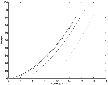
FIG. 6.: The soliton dispersions, plotted in a frame in which $\sum_{n=1}^{N-1}k_{n}=0$. For $\eta>2$ all the curves lie on top of each other; they are shown by the solid line. The dashed line is for $\eta=2$ when they just start peeling apart. The dashdot line and the dotted line are for $\eta=0.1$ and $\eta=0.01$ respectively. The energies are in units of $\eta$, i.e. the Hamiltonian (3), in terms of $\hbar$, is used.

Finally, if we wish to compare our system to the free Fermi gas which it resembles in one limit, we could look at the “particle-hole excitation spectrum” commonly plotted for such systems. To do this we start from the ground state, with contiguous $I_{n}$; pick up one of these, say $I_{m}$, move it to $I^{\prime}_{m}$ (where $I^{\prime}_{m}>I_{N}$ since all other states are occupied), and define the momentum of this “particle-hole excitation” as $Q=2\pi(I^{\prime}_{m}-I_{m})/N$. (This is basically the total phonon momentum of such an excitation.) Then one gets a one-parameter range of energies for every $Q$, as shown in Fig. 7. The harmonic and $\eta\rightarrow 0$ limits look similar, qualitatively; the phonon or hole branch (the lower edge for $Q<2\pi$) is a sine curve in the former case and a parabola in the latter, and the particle branch (the upper edge and the lower edge for $Q>2\pi$) is a straight line in the harmonic limit and a curve (which indicates nonlinearity) otherwise. The upper edge of the particle hole continuum has been identified with a “soliton” by Sutherland, and corresponds to promoting $k_{N}$ from the ground state configuration to one with a larger value, and is thus essentially identical to our picture explained above. A study of the quantum numbers of the solitons and the phonons leads to a suggestive “phonon decomposition” of the soliton: we can view the soliton creation operator $A_{q}$ schematically in terms of a phonon creation operator $a^{\dagger}_{q}$ as

$$A^{\dagger}_{\frac{2\pi}{N}m}\;\;\sim\;\;[a^{\dagger}_{\frac{2\pi}{N}}]^{m},$$ (72)

i.e. a particular kind of highly symmetric multi phonon state.

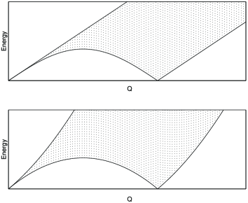
FIG. 7.: Particle-hole excitations. In between the bounding upper and lower curves lies a continuum of allowed energy values corresponding to each $Q$ where $Q$ is as defined in §VII for a single particle-hole pair. The upper graph corresponds to the harmonic limit, the lower graph to the $\eta\rightarrow 0$ limit. (The energy scales are different in the two graphs.)

VIII Correlation Functions, Finite-size Effects and Conformal Theory

We now turn to the issue of correlation functions of the Toda lattice, making contact with the the theory of conformal invariance in this class of systems. Conformal invariance has given considerable insight into correlation functions of quantum many body models having critical behaviour, as typified by a vanishing of excitation energies or power law correlations, and useful reviews of this fast growing field are to be found in [16] and in [17].

Let us first note that the quantum Toda lattice in its ground state is not quite a lattice: the Bragg peaks are melted due to zero point motion. In the harmonic limit this is simple to see, since we can write the displacement in terms of the phonon creation operators and the phonon dispersion $\omega_{q}=2\;v\;|\sin(q/2)|$ as

$$u_{n}=\frac{1}{\sqrt{N}}\sum_{q}\;\exp(iqn)\;\;\frac{1}{i\sqrt{\omega_{q}}}\;\;(a^{\dagger}_{q}-a_{-q})$$ (73)

whereby $\left<u^{2}_{n}\right>=(1/N)\sum(1/\omega_{q})\;\sim(1/\pi v)\log(N)$. The phonon velocity $v=\sqrt{2\eta}$ in the harmonic limit of the Toda problem. The structure function at the first reciprocal lattice vector $G=(2\pi/N)$ is

$$\left<\rho_{G}\;\;\rho_{G}\right> = \sum_{m,n}\left<e^{i2\pi u_{n}}\;\;e^{-i2\pi u_{m}}\right>$$ (74)

$$\left<e^{i2\pi u_{n}}\;\;e^{-i2\pi u_{m}}\right> = e^{-2\pi^{2}\langle(u_{n}-u_{m})^{2}\rangle}=e^{-4\pi/v\log(|m-n|)}$$ (75)

$$= \frac{1}{|m-n|^{4/\pi v}}$$ (76)

where we have used the Gaussian cumulant theorem $\left<\exp(a)\right>=\exp(1/2\left<a^{2}\right>)$ and the logarithmic integral $(1/N)\sum(1-\cos(qr))/\omega_{q}\sim(1/\pi v)\log(r/r_{0})$. We thus see that the Toda lattice may be expected to have powerlaw correlations for all $\eta$, since it has low energy excitations for all $\eta$, namely the phonons.

A characteristic of conformally invariant theories is the ‘central charge’ $c$. One way of checking for conformal invariance is to compute corrections to the ground state energy for a finite sized system, which is expected to have a behaviour

$$E(L)=Le_{\infty}-\frac{c\pi v}{6L}+O(1/L^{2})$$ (77)

where $v$ is the velocity of the low lying excitations, such that a tower of excited states exists with energy $v2\pi/L\times\mbox{integer}$. A glance at (52) shows that in that limit of large $\eta$ we have $c=1$, as indeed does the initial $1/\sinh^{2}$ model. The case of $c=1$ usually leads to exponents varying continuously with coupling constants, and hence (76) is consistent with this possibility. In the present model, we must, however, first establish that the asymptotic Bethe ansatz gives the correct energy to O($1/N$) or O($1/L$). This is not guaranteed a priori by any theoretical argument and must be checked for self consistency. (Incidentally, in the Toda lattice we are at a fixed density so we will not distinguish between $L$ and $N$.) The internal check performed is to compute the velocity at a fixed $\eta$ and to compute the energy for various $N$ and to check against Eq. (77).

First we note that in the extreme anharmonic limit equation (57) for the ground state in the low $\eta$ limit does indeed give the same sound velocity as (63) or (64), so in the low $\eta$ limit $c=1$ exactly, as it is in the harmonic limit.

We performed the calculation for $\eta=2,10,100$ (Table I). As in figures 2 and 3, we use the Hamiltonian (3) and units of $\hbar$ (equivalently, the Hamiltonian (1) with units of $\sqrt{2\eta}$); in these units the sound velocity for the harmonic lattice is 1 exactly. From these results, we get

$vc=$	$1.0764\pm 0.0006$	($\eta=2$)
	$1.035\pm 0.003$	($\eta=10$)
	$1.01\pm 0.03$	($\eta=100$)

On interpolating the 19-particle results of Fig. 3 for q=0, we get the estimates $v=1.08,1.04,1.01$ for $\eta=2,10,100$ respectively, with uncertainties in the second decimal place. Thus we get for the central charge

$c=$	$1.00\pm 0.01$	($\eta=2,10$)
	$1.00\pm 0.03$	($\eta=100$).

The uncertainty in the cases $\eta=2$, $10$ arises mainly from the inaccuracy in our determination of $v$. The results seem to indicate that $c$ is equal to 1 at all values, and moreover it is reproduced correctly by the Bethe ansatz even at $\eta=100$, which is well into the “classical” limit. It thus appears that the error in energy per particle goes, at worst, as the inverse cube of the number of particles. The error bars could be reduced by increasing the system size further.

In the anharmonic limit, in fact, the series stops there ($E/N$ has only a constant piece and a $1/N^{2}$ piece) while in the harmonic limit all odd powers, $1/N^{3}$, $1/N^{5}$ and so on are missing. One might conjecture that this is the case at all values of $\eta$. For $\eta=2$ we took the ground state energies per particle for various $N$, subtracted $e_{\infty}$ and the $1/N^{2}$ piece, and fitted the results to power series in $1/N$ starting at $N^{-3}$. The result was a coefficient of $0.021\pm 0.006$ for the $N^{-3}$ term, and $-1.1\pm 0.2$ for the $N^{-4}$ term. Thus the coefficient of the $1/N^{3}$ term does seem to be very nearly zero. For $\eta=10$ and $100$ the numbers we obtained didn’t allow us to make such fits—the error bars turned out to be much larger than the values themselves. We conjecture that the coefficient of the $1/N^{3}$ term vanishes at all $\eta$, but for high $\eta$ the Bethe ansatz may not be accurate to this order in $N$ and may be unable to reproduce this result. We are unable to make a statement about higher odd powers.

TABLE I.: Ground state energy per particle as a function of system size

N		$E/N$
	$\eta=2$	$\eta=10$	$\eta=100$
29	1.675512397777	2.890224040772
33	1.675665073759	2.890370838890
41	1.675847391894	2.890546128059
49	1.675947956073	2.890642813964
57	1.676009234239	2.890701728785	7.713369630480
65	1.676049312911	2.890740261674	7.713407380691
81			7.713452036110
97			7.713476466168
113			7.713491273955
129			7.713500922044

Accepting that the Toda lattice is a $c=1$ theory, we can establish the power law of the density correlator as in (76), without too much detailed calculation, on using the Galilean invariance of the model. The theory of conformal invariance (see e.g. [17]) says that if we have an excitation that boosts the total momentum by $k_{tot}$ then the change in energy is

$$\delta E = 2\pi vx/N$$ (78)

$$x = (\frac{k_{tot}}{2\pi})^{2}\mu$$ (79)

$$\alpha = 2\mu$$ (80)

where $\alpha$ is the exponent determining the decay of a primary operator. However, Galilean invariance implies that

$$\delta E=\frac{k_{tot}^{2}}{N};$$ (81)

hence we find

$$\alpha=\frac{4\pi}{v}.$$ (82)

Comparing with the harmonic limit result (76), we see that the primary operator may be identified with the density fluctuation $\rho_{G}$ and hence the result (76) is true at all $\eta$ provided we substitute the appropriate value of $v(\eta)$. A similar result is well known to be true for the $1/r^{2}$ models for the density correlation function, but unlike in that case, there is a difficulty in defining a “bosonic” correlator, since we are always working at a fixed density, and hence the compressibility is zero.

IX Comparison with the classical Kac - Van Moerbeke formulation

To summarize the above, we now have a picture of how the $k$’s in the Bethe ansatz (or the $\rho$’s in Gutzwiller’s treatment) behave, in the ground state and in the excited states. In the ground state the $I$’s and therefore the $k$’s are all closely spaced. In the excited states the separations between them widen. If there is a gap of $m$ integers between $I_{N-n}$ and $I_{N-n+1}$ the gap between $k_{N-n}$ and $k_{N-n+1}$ widens and one has $m$ phonons in the $n$th normal mode. If the gap between the $k$’s becomes very large the excitation becomes solitonic. In particular, for $n=1$ one has a one-soliton state; for $n=2$, a two soliton state (with equal amplitudes); and so on.

We now compare this description with the description of the system in the classical variables of Kac and van Moerbeke [5, 3]. Briefly they use the variables $\mu_{1},\mu_{2},\ldots,\mu_{N-1}$ which are the eigenvalues of a truncated Lax matrix obtained by striking off the first row and column (i.e. removing the first particle from the problem). These $\mu$’s are the momenta of the particles in the remaining open chain if the system is dilute. Kac and van Moerbeke show that these $\mu$’s are confined to the $N-1$ closed intervals where the characteristic polynomial of the Lax matrix, $\left|\lambda I-L\right|$ is equal to or greater than 2 in magnitude. The polynomial goes to $\pm\infty$ for large $\lambda$, while it oscillates in the middle; for the ground state it touches the lines $\lambda=\pm 2$ in $N-1$ places so that the closed intervals referred to above are single points and all the $\mu$’s are stationary. For an excited state the polynomial crosses the lines $\lambda=\pm 2$ so the closed intervals get a finite width and the $\mu$’s oscillate inside these intervals as the system evolves.

The analogues of the classical $\mu$’s are Gutzwiller’s $\rho$’s, or approximately Sutherland’s $k$’s. Whereas there are $N-1$ $\mu$’s each confined to a different interval in the classical picture, in Gutzwiller’s picture each of the $N-1$ analogous variables has a spectrum of $N$ values $\rho_{n}$. On calculating the classical $\mu$’s in the ground state, as is done in [3], we find that their values lie almost exactly in between the quantum $\rho$ (ie $k$) values. There is an analogy between the $\mu$’s and the “gaps” in the $k$-spectrum. In the ground state the gaps are minimum, the $\mu$’s fit into these gaps, and the $\mu$’s are stationary. In an excited state some or all of these gaps between the $k$’s widen, and the corresponding $\mu$’s are no longer stationary but oscillate in intervals of finite width. In particular a pure cnoidal wave corresponds to exactly one $\mu$ acquiring a width in which to oscillate, or exactly one gap among the $I_{n}$ (hence the $k_{n}$) widening.

A single cnoidal wave has the formula [3]

$$e^{-r_{n}}=1+(2K\nu)^{2}\left(\mbox{dn}^{2}\left[2(n/\lambda\pm\nu t)K\right]-E/K\right),$$ (83)

where $r_{n}=u_{n}-u_{n-1}$, $K$ and $E$ are the complete elliptic integrals of the first and the second kind, $\lambda$ is the wavelength ($=N$ for the first “normal mode” or one soliton, $N/2$ for the second normal mode, etc) and $\nu$ is given by

$$2K\nu=\left[\frac{1}{\mbox{sn}^{2}(2K/\lambda)}-1+\frac{E}{K}\right]^{-1/2}$$ (84)

For low modulus $k$ of the elliptic functions, this is like a sinusoidal wave, but as the modulus increases it becomes sharply peaked locally and flat elsewhere (Fig. 1). As remarked in §VII, the dispersion calculated from this expression is close to the dispersion, in an appropriate reference frame, of the quantum cnoidal wave.

X Conclusions

In conclusion, we have shown that the usefulness of the asymptotic Bethe ansatz in the quantum Toda problem is not confined to finding thermodynamic properties. The method gives results for energy per particle accurate to O($1/N^{2}$), which is sufficient to calculate finite size effects and even correlation functions using conformal theory. The O($1/N^{3}$) term seems to vanish in the exact solution, though the Bethe ansatz solution probably doesn’t reproduce this result.

We have demonstrated that in fact the Bethe ansatz equations are a simplification of Gutzwiller’s method and can be derived from them. The parameter governing the error can be taken to be the difference in $\rho_{n}$ and $\epsilon_{n}$ in §IV. According to Matsuyama [14] this difference falls exponentially with $N$, so that the error goes as $e^{-N/f(\eta)}$, where $f(\eta$) is some dimensionless number. We also show that the error vanishes as $\eta$ becomes small, so that $f(\eta)\rightarrow 0$ as $\eta\rightarrow 0$.

Thus, we can treat finite sized systems, account for low-lying states (phonons) and higher excitations (solitons), and find their dispersions and velocities. Comparison with conformal theory gives the “central charge” $c=1$, which means that the coefficient of the $1/N^{2}$ term in the $E/N$ expansion is essentially the sound velocity.

We find that the properties of excitations are very similar to the classical properties for $\eta>2$ ($\hbar<1$), apart from the underlying discreteness of the energy levels. The quantization is then analogous to the quantization of a harmonic lattice. The soliton, which is an effect of large occupation of one mode, is no different from the classical object described by Toda; even its energy is effectively not quantized since the occupation number is so large.

For small $\eta$ (large $\hbar$) things are different: the phonons no longer derive from a harmonic approximation, and the soliton dispersions no longer match the classical ones, though qualitatively the dispersion curves retain some similar features, both for solitons (high-amplitude cnoidal waves) and for phonons. For both excitations the dispersions depend on $\eta$, and moreover the energy of a mode deviates rapidly from linearity with increasing occupation number $n$, so that $n$ need not be macroscopic (at least for finite lattice size $N$) for the mode to become soliton-like—the soliton’s energy is indeed quantized. Thus if the large $\eta$ soliton is essentially the soliton of Toda’s classical lattice, the corresponding small $\eta$ object deserves to be called the quantum soliton.

Hénon’s integrals, classical and quantum

In this appendix we discuss the integrability of the Toda lattice classically and quantum mechanically; while much of the discussion is not new it seems difficult to find it in one place elsewhere. Following Pasquier and Gaudin [9], who give a proof of quantum integrability, we show that their conserved quantities are the same as Hénon’s integrals—whose conservation is necessary for Gutzwiller’s treatment to go through.

The equations of motion for the classical lattice can be written in the Lax form

$$\frac{dL}{dt}=LM-ML,$$ (85)

where

$$L=\left(\begin{array}[]{ccccc}b_{1}&a_{1}&&&a_{N}\\ a_{1}&b_{2}&a_{2}\\ &a_{2}&b_{3}\\ &&&\ddots&a_{N-1}\\ a_{N}&&&a_{N-1}&b_{N}\end{array}\right),$$ (91)

$$M=\left(\begin{array}[]{ccccc}0&a_{1}&&&-a_{N}\\ -a_{1}&0&a_{2}\\ &-a_{2}&0\\ &&&\ddots&a_{N-1}\\ a_{N}&&&-a_{N-1}&0\end{array}\right)$$ (97)

and

$$a_{j}=e^{-(q_{j_{1}}-q_{j})/2},~{}~{}~{}b_{j}=p_{j}.$$ (98)

From this one can show that the eigenvalues of the Lax matrix $L$, or equivalently the coefficients $I_{n}$ of the characteristic polynomial of the Lax matrix are conserved quantities [3]. These are Hénon’s integrals, and are given by

$$I_{m}=\sum_{{i_{1},i_{2},\ldots,i_{k},}\atop{j_{1},j_{2},\ldots,j_{l}}}p_{i_{1}}p_{i_{2}}\ldots p_{i_{k}}\left(-X_{j_{1}}\right)\left(-X_{j_{2}}\right)\ldots\left(-X_{j_{l}}\right)$$ (99)

where

$$X_{j}=e^{-(q_{j+1}-q_{j})},$$ (100)

there are no repeated indices in the $p$’s or the $q$’s in a given term ($i_{1}$, $i_{2}$, …, $j_{1}$, $j_{1}+1$, $j_{2}$, $j_{2}+1$, …are all different), the total number of such indices in each term is $m$ (i.e. $k+2l=m$) and the sum is over all distinct terms satisfying these conditions (i.e. terms not differing merely in the order of factors).

In quantum mechanics, the coefficients of the Lax matrix are the same, and have no ordering problems, but now the equations of motion (85) are no longer valid (each term in the matrix product has to be ordered) and the proof that the coefficients are conserved fails. Gutzwiller [7] assumes that they are conserved nonetheless (he only takes the cases $N=3,4$ where it can be verified easily). Their conservation can be shown as a consequence of the work of Pasquier and Gaudin [9], who prove that the coefficients of $u$ in the trace of the “monodromy matrix” $T_{N}$ are in involution, where

$$T_{N}(u) = L_{1}L_{2}\ldots L_{N},$$ (101)

$$L_{n}(u) = \left(\begin{array}[]{cc}u-p_{n}&\;e^{q_{n}}\\[5.0pt] -e^{-q_{n}}&\;0\end{array}\right).$$ (104)

The definitions hold in both the classical and the quantum cases. Classically their conservation follows from the classical equations of motion

$$\frac{dL_{n}}{dt} = M_{n-1}L_{n}-L_{n}M_{n},$$ (105)

$$\mbox{where}~{}~{}M_{n} = \left(\begin{array}[]{cc}u&\;e^{q_{n}}\\[5.0pt] -e^{-q_{n+1}}&\;0\end{array}\right).$$ (108)

Quantum mechanically these satisfy the Yang-Baxter equations: we may rewrite $L_{n}\rightarrow L_{n,g}(u)=(u-p_{n})(1+\sigma_{g}^{z})/2-\exp(-q_{n})\;\sigma_{g}^{-}+\exp(q_{n})\;\sigma_{g}^{+}$ and show that the monodromy matrix $T_{N}(u)\rightarrow T_{g}(u)$ satisfies the Yang-Baxter condition $T_{g}(u)T_{g^{\prime}}(v)R_{g,g^{\prime}}(u-v)=R_{g,g^{\prime}}(u-v)T_{g^{\prime}}(u)T_{g}(v)$ with $R_{g,g^{\prime}}=a(u-v)+b(u-v)\vec{\sigma_{g}}.\vec{\sigma_{g^{\prime}}}$. Taking a trace over the auxiliary spaces $\sigma_{g},\sigma_{g^{\prime}}$ the integrability is established. We now show that these coefficients are in fact Hénon’s integrals. Consider a polynomial in $u$, $F_{N}(u)$, defined by

$$F_{N}(u)=\sum^{k+2l=N} (u-p_{i_{1}})(u-p_{i_{2}})\ldots(u-p_{i_{k}})$$ (110)

$$\ldots(-X_{j_{1}})(-X_{j_{2}})\ldots(-X_{j_{l}})$$

where the indices satisfy the same restrictions as in the definition of Hénon’s integrals. It is easily seen that

$$F_{N}(u)=\sum_{n=0}^{N}(-1)^{n}I_{n}u^{N-n}.$$ (111)

We can show by induction that this polynomial is the trace of $T_{N}(u)$. Defining

$$F^{\prime}_{N}(u) = F_{N}(u)$$ All the terms in (113)

$$\mbox{ which do not include a factor $e^{q_{N}}$},$$

$$F^{\prime\prime}_{N}(u) = F_{N}(u)-F^{\prime}_{N}(u)$$ (114)

$$= F_{N}(u)$$ All the terms in (116)

$$\mbox{ which include a factor $e^{q_{N}}$},$$

we claim that

$$T_{N}=\left(\begin{array}[]{cc}F^{\prime}_{N}(u)&\;e^{q_{N}}F^{\prime}_{N-1}(u)\\[10.00002pt] e^{-q_{N+1}}F^{\prime\prime}_{N+1}(u)&\;F^{\prime\prime}_{N}(u)\end{array}\right).$$ (117)

The claim is easily verified for $N=1,2,$ etc. Suppose it is true for $N$; then

$$T_{N+1}=T_{N}L_{N+1}=$$ (118)

$$~{}~{}\left(\begin{array}[]{cc}(u-p_{n+1})F^{\prime}_{N}(u)&e^{q_{N+1}}F^{\prime}_{N}(u)\\ -e^{q_{N}-q_{N+1}}F^{\prime}_{N-1}(u)&\\[15.00002pt] (u-p_{N+1})e^{-q_{N+1}}F^{\prime\prime}_{N+1}(u)&F^{\prime\prime}_{N+1}(u)\\ -e^{-q_{N+1}}F^{\prime\prime}_{N}(u)&\end{array}\right)$$ (123)

which one can check is the same as

$$T_{N+1}=\left(\begin{array}[]{cc}F^{\prime}_{N+1}(u)&e^{q_{N+1}}F^{\prime}_{N}(u)\\[10.00002pt] e^{-q_{N+2}}F^{\prime\prime}_{N+2}(u)&F^{\prime\prime}_{N+1}(u)\end{array}\right).$$ (124)

Thus our claim is true for all $N$, and in particular the trace of $T_{N}$ is $F_{N}(u)$.

REFERENCES

- [1] email: rsidd@physics.iisc.ernet.in
- [2] email: bss@physics.iisc.ernet.in
- [3] M. Toda, Theory of Nonlinear Lattices, second edition, Springer Series in Solid State Sciences 20 (Berlin:Springer 1988)
- [4] M. Toda, J. Phys. Soc. Japan 23, 501 (1967)
- [5] M. Kac and P. van Moerbeke, Proc. Nat. Acad. Sci. USA 72, 1627 (1975); 72, 2879 (1975)
- [6] E. Date and S. Tanaka, Prog. Theor. Phys. 55, 457 (1976); Prog. Theor. Phys. Suppl. 59, 107 (1976)
- [7] M. Gutzwiller, Ann. Phys. 133, 304 (1981)
- [8] E. K. Sklyanin, in Nonlinear Equations in Classical and Quantum Field Theory (ed. N. Sanchez), Lecture Notes in Physics 226, Springer-Verlag, Berlin (1985)
- [9] V. Pasquier, M. Gaudin, J. Phys. A 25, 5243 (1992)
- [10] B. Sutherland, Rocky Mountain J. Math. 8, 413 (1978)
- [11] F. G. Mertens, Z. Phys. B 55, 353 (1984); M. Hader and F. G. Mertens, J. Phys. A, 19, 1913 (1986)
- [12] M. Fowler and H. Frahm, Phys. Rev. B 39, 16, 11800 (1989)
- [13] B. Sutherland, in Exactly Solvable Problems in Condensed Matter and Relativistic Field Theory (ed. B. S. Shastry, S. S. Jha and V. Singh), Lecture Notes in Physics 242, Springer-Verlag, Berlin (1985)
- [14] A. Matsuyama, J. Phys. A 29, 1089 (1996)
- [15] A. Matsuyama, Ann. Phys. 220, 300 (1992)
- [16] P. Christe and M. Henkel, Introduction to Conformal Invariance and its Applications to Critical Phenomena, Lecture Notes in Physics m 16, Springer-Verlag, Berlin (1993).
- [17] N. Kawakami, Prog. Theor. Phys. 91, 189 (1994).