[

Quantum Versus Mean Field Behavior of Normal Modes of a Bose-Einstein Condensate in a Magnetic Trap

Abstract

Quantum evolution of a collective mode of a Bose-Einstein condensate containing a finite number $N$ of particles shows the phenomena of collapses and revivals. The characteristic collapse time depends on the scattering length, the initial amplitude of the mode and $N$. The corresponding time values have been derived analytically under certain approximation and numerically for the parabolic atomic trap. The revival of the mode at time of several seconds, as a direct evidence of the effect, can occur, if the normal component is significantly suppressed. We also discuss alternative means to verify the proposed mechanism.

PACS numbers: 03.75.Fi, 05.30.Jp, 32.80.Pj, 67.90.+z

]

The progress [1, 2, 3, 4] in trapping the low density alkaline gases and cooling them below the temperature $T_{BEC}$ of the Bose-Einstein condensation has initiated a search for features of the atomic coherent collective behavior specific for the trapped condensate. The theoretical predictions [5, 6, 7] made for the normal frequencies of the condensate in the traps have been successfully confirmed in the experiments [8, 9] employing the resonant modulations of the trapping potential.

It is worth noting that the calculations of the normal frequencies [5, 6, 7] are based on the Gross-Pitaevskii (GP) equation strictly valid in the limit of a number of particles $N\to\infty$, with the average density $\rho$ being fixed [10]. The GP equation describes the condensate in the mean field (MF) approximation. In this sense the condensate wave function $\Phi({\bf x},t)$ obeying the time dependent GP equation is viewed as a classical field [10]. In the atomic traps [1, 2, 3, 4] neither $N$ can be obviously considered as infinite nor $\rho$ is fixed ($\rho\sim N$ for $N<200-500$ and $\rho\sim N^{2/5}$ for $N>10^{4}$ [11]). Therefore, it is important to understand how the actual quantum evolution of the collective mode deviates, if any, from that predicted by the mean field approach for finite $N$.

In this paper we will show that, while the normal frequencies and short time evolution are determined correctly by the GP equation whenever $N$ is only a few times larger than 1, the quantum behavior of the normal modes can deviate from the mean field one at times much longer than the time scale set by the normal frequencies. The quantum behavior is characterized by dephasing, that is by the phenomena of the collapses and the revivals of the normal mode amplitude at zero temperature. Below we will derive the corresponding quantum solution in the approximation neglecting the exchange effects. The numerical solution taking into account the full many body Hamiltonian for $N=300$ in the approximation allowing $N$ atoms to occupy two single particle levels only is presented also. It turns out that both approaches yield close values for the collapse and the revival times, respectively, with the collapse time being of the same order of magnitude as the relaxation time reported experimentally [8, 9].

The quantum collapses and revivals were first analyzed in Ref.[12] for a single atom in a resonant cavity. Very recently such phenomena have been observed experimentally [13]. As was suggested in Refs.[14, 15], the phase of the condensate containing finite numbers of particles in their ground state should also undergo the same phenomena. In this case, however, the one-particle density matrix remains insensitive to such fluctuations. Consequently, special arrangements of at least two condensates are required in order to detect this effect [14, 16].

In contrast, for the condensate collective mode the situation is less restrictive. The collapses and revivals of the collective mode of the condensate with fixed $N$ can be detected by the one-particle density matrix at zero temperature. A physical reason for this effect is the following: For fixed finite $N$ a collective mode is represented by a multiple mixture of the eigenstates rather than by a single eigenstate of the $N$-body Hamiltonian. In general, the inter particle interaction makes the eigenenergies dependent nonlinearly on the quantum numbers of the Fock space. Under such circumstances the quantum beats develop resulting in collapses and revivals [17]. For $N\to\infty$, this mixture approaches the coherent state and can become a true eigenstate of the Hamiltonian. Accordingly, in such a limit the beats should vanish. It is worth noting that in the atomic traps the existence of this limit is nontrivial because of the dependence of $\rho$ on $N$.

Within the Hartree approach excitations of a Bose-Einstein condensate can be described by the GP equation [10, 5, 6, 7] $i\dot{\Phi}=\delta E^{(\Phi)}/\delta\Phi^{*}$ for the classical field $\Phi({\bf x},t)$ which represents the Hartree many body wave function $|\Phi\rangle$ for $N$ bosons. Here $E^{(\Phi)}=\langle\Phi|H|\Phi\rangle$ is the GP energy functional obtained from the second quantized Hamiltonian

$$H=\int d{\bf x}[\Psi^{\dagger}(H_{1}-\mu)\Psi+{u_{o}\over 2}\Psi^{\dagger}\Psi^{\dagger}\Psi\Psi]$$ (1)

by replacing the Bose operator $\Psi$, obeying the usual Bose commutation rule, by the classical field $\Phi$ [10]. As usual, in Eq.(1) $H_{1}$ is the single particle Hamiltonian; $u_{0}$ denotes the interaction constant (we express $u_{0}=4\pi a/M$ by means of the positive scattering length $a$ and the atomic mass $M$ in units where $\hbar=1$); $\mu$ is the chemical potential. In fact, the replacement of the operator $\Psi$ by $\Phi$ is equivalent to projecting of the full many body wave function $|\Psi\rangle$ to the Hartree (MF) ansatz [18]

$$|\Phi\rangle={(\sum_{k}C^{*}_{k}(t)a^{\dagger}_{k})^{N}|0\rangle\over\sqrt{N!}},\,\sum_{k}C^{*}_{k}(t)C_{k}(t)=1,$$ (2)

with $C_{k}(t)$ being $c$-numbers and $|0\rangle$ standing for the vacuum state. In (2) $a^{\dagger}_{k},a_{k}$ are creation and annihilation operators, respectively, for a particle at the single particle state $\psi_{k}({\bf x})$. For the most general representations of the classical field $\Phi({\bf x},t)=\sum_{k}C_{k}(t)\psi_{k}({\bf x})$ and the Heisenberg operator $\Psi({\bf x},t)=\sum_{k}a_{k}(t)\psi_{k}({\bf x})$, the replacement procedure and calculating the mean $\langle\Phi|H|\Phi\rangle$ for the state (2) yield the same GP functional $E^{(\Phi)}$ from the Hamiltonian (1) when $N$ is only a few times larger than 1.

In what follows we will compare predictions for the time evolution of the normal modes provided by the mean field approach with the full quantum mechanical calculations which do not rely on the projection to the states (2). A good qualitative description of the quantum evolution is provided by the following two-level model: $N$ bosons can occupy two one particle states, one given by the function $\psi_{0}({\bf x})$ minimizing the Hartree energy in the ground state and the other given by the function $\psi_{1}({\bf x})$ which is orthogonal to $\psi_{0}({\bf x})$. Both functions are taken orthonormal $\int d{\bf x}\psi^{*}_{i}\psi_{j}=\delta_{ij}$. Keeping $i,j=0,1$ only restricts the space of states available for each particle. In this manner, we neglect the processes of interaction of the collective mode under consideration, which corresponds to transitions between states $\psi_{0}({\bf x})$ and $\psi_{1}({\bf x})$, with the rest of other modes. Note that the interaction with other modes, ascribed to transitions to states $\psi_{k}$ with $k>1$, is sensitive to the square of the mode amplitude, while the rate of the dephasing, as it will be shown, depends linearly on the amplitude. Therefore, for the small amplitude the dephasing effect will dominate.

The choice of $\psi_{0}({\bf x})$ is dictated by the requirement that the Hartree variational energy of the ground state is minimal for $C_{0}=1$ (and $C_{k}=0$ for $k>0$) in (2). Taking into account Eqs.(1),(2) and minimizing $E^{(\Phi)}$ with respect to $\Phi=\psi_{0}$, one obtains the GP equation

$$(H_{1}-\mu)\psi_{0}+u_{0}N|\psi_{0}|^{2}\psi_{0}=0.$$ (3)

The choice of $\psi_{1}({\bf x})$, however, depends on the characteristic of the collective mode being studied as well as the magnitude of its frequency [19]. In what follows we will employ the Schrödinger representation relying on the time-independent operator $\Psi$. Substituting $\Psi=a_{0}\psi_{0}({\bf x})+a_{1}\psi_{1}({\bf x})$ in Eq.(1), one obtains the second quantized Hamiltonian (1) rewritten as

$$\begin{array}[]{l}H=(\varepsilon_{00}-\mu)a^{\dagger}_{0}a_{0}+(\varepsilon_{11}-\mu)a^{\dagger}_{1}a_{1}+[(\varepsilon_{10}+\\ \\ v(t))a^{\dagger}_{1}a_{0}+h.c.]+{1\over 2}\sum_{i,j,k,l}u_{ijkl}a^{\dagger}_{i}a^{\dagger}_{j}a_{k}a_{l},\end{array}$$ (4)

where $u_{ijkl}=u_{0}\int d{\bf x}\psi^{*}_{i}\psi^{*}_{j}\psi_{k}\psi_{l}$ ($i,j,k,l=0,1$); $\varepsilon_{ij}=\int d{\bf x}\psi^{*}_{i}H_{1}\psi_{j}$. We have also introduced the term $\sim v(t)$ which models the effect of the modulation of the trapping potential employed in Refs. [8, 9] to excite the condensate normal modes. In what follows we assume that $\psi_{i}$ are chosen in a manner which yields $u_{ijkl}$ real. This, in turn, implies the condition $u_{ijkl}=u_{klij}$.

If the total number of particles $N$ is fixed, the Hamiltonian (4) becomes a $N+1$ by $N+1$ Hermitian matrix $H_{n,m}=\langle N-n,n|H|m,N-m\rangle$ in the Fock space $|n,N-n\rangle$ where $n=0,1...N$ denotes the number of atoms at the level $1$, with $N-n$ atoms remaining on the level $0$. Correspondingly, the Schrödinger equation for the many body wave function in the Fock representation $|\Psi\rangle=\sum^{N}_{n=0}B_{n}(t)|n,N-n\rangle,\,\sum^{N}_{n=0}|B_{n}|^{2}=1$ is

$$i\dot{B}_{n}=\sum^{N}_{m=0}H_{n,m}B_{m},$$ (5)

where explicitly the nonzero elements ($H_{n,m}^{*}=H_{m,n}$) are $H_{n,n}=\varepsilon n+g_{1}n^{2}/2$, $H_{n,n-1}=\sqrt{n(N-n+1)}[v(t)+(u_{1110}-u_{1000})(n-1)]$, and $H_{n,n-2}=u_{1100}\sqrt{n(n-1)(N-n+1)(N-n+2)}/2$. Here the notations $g_{1}=u_{0000}+u_{1111}-4u_{1010}$, $\varepsilon=\varepsilon_{11}-\varepsilon_{00}+(u_{0000}-u_{1111})/2+(2u_{1010}-u_{0000})N$ are introduced, and the overall constant in $H_{n,n}$ is omitted to set $H_{0,0}=0$. Note that the term $g_{1}n^{2}/2$ in $H_{n,n}$ is due to the interparticle interaction. This describes the effect of renormalizing of the ideal gas spectrum $\varepsilon n$ in the lowest order with respect to the scattering length $a$. We have also made use of the relation $\varepsilon_{10}+Nu_{1000}=0$ obtained by means of multiplying Eq.(3) by $\psi_{1}^{*}$ and integrating over $\bf x$, given the condition $\int d{\bf x}\psi^{*}_{1}\psi_{0}=0$. The condensate in this model is associated with the ground eigenstate of the Hamiltonian matrix in Eq.(5) for $v=0$. The one particle density matrix $\rho({\bf x},{\bf x^{\prime}},t)=\sum_{i,j}\rho_{ij}(t)\psi^{*}_{i}({\bf x})\psi_{j}({\bf x^{\prime}})$, with $\rho_{ij}(t)=\langle\Psi|a^{\dagger}_{i}a_{j}|\Psi\rangle$ ($\rho_{ij}(t)=\rho_{ji}^{*}(t)$), is given explicitly by

$$\begin{array}[]{l}\rho_{00}(t)=N-\rho_{11}(t),\,\rho_{11}(t)=\sum^{N}_{n=0}n|B_{n}(t)|^{2},\\ \\ \rho_{10}(t)=\sum^{N}_{n=0}\sqrt{(n+1)(N-n)}B_{n+1}(t)^{*}B_{n}(t).\end{array}$$ (6)

Note that the corresponding MF expression for the density matrix is $\rho^{(\Phi)}_{ij}(t)=\langle\Phi|a^{\dagger}_{i}a_{j}|\Phi\rangle=NC^{*}_{i}(t)C_{j}(t)$, where the Hartree ansatz (2) has been employed and $C_{i}(t)$ must be found from the GP equation $i\dot{C}_{i}=\delta E^{(\Phi)}/\delta C^{*}_{i}$ in the restricted basis $\psi_{0},\,\psi_{1}$

$$i\dot{C}_{i}=\sum_{j}(\varepsilon_{ij}+v_{ij}-\mu\delta_{ij})C_{j}+N\sum_{jkl}u_{ijkl}C^{*}_{j}C_{k}C_{l}.$$ (7)

Here $i,j,k,l=0,1$; also we have introduced the notations $v_{10}=v_{01}^{*}=v(t)$. This system describes the evolution of the Hartree state (2) [18] which is expected to be very close to the actual state for the case $N\to\infty$ and $\rho$ fixed [10]. For finite and large $N$ one can expect that the classical and the quantum solutions do not differ much at short times. Therefore, it is natural to assume that the driving term $v(t)$ in Eq.(7) prepares the state (2) (at $t=0$) with some $C_{k}(0)$ and then is removed so that the quantum evolution at $t=0$ starts from the state (2), with $v(t)=0$ for $t>0$. This provides the initial condition $|\Psi(t=0)\rangle=|\Phi(t=0)\rangle$. Comparing (2) with the full Fock state $|\Psi\rangle$, one finds

$$B_{n}(0)=\sqrt{\frac{N!}{n!(N-n)!}}\left(C_{0}^{N-n}(0)C_{1}^{n}(0)\right)^{*}.$$ (8)

We consider first an approximation when $\rho_{ij}(t)$ can be found analytically. Specifically, we ignore the off-diagonal terms of the Hamiltonian (5) which correspond to the exchange of atoms between the states 0, 1 in the representation (4). Below it will be seen that this approximation provides qualitatively correct results when these exchange terms are smaller than the term $\varepsilon n$ in $H_{n,n}$ (5). In future work we will show how this approximation can be extended for the case of larger values of the off-diagonal terms. Correspondingly, one has $B_{n}(t)=B_{n}(0){\rm exp}(-iH_{n,n}t)$. This results in Eq.(6) rewritten as $\rho_{00}=N|C_{0}(0)|^{2}=$const, $\rho_{11}=N|C_{1}(0)|^{2}=$const and

$$\begin{array}[]{ll}\rho_{10}(t)&=N\rho_{1}\exp(-i(\varepsilon+g_{1}/2)t)\\ &\cdot\left(1+|C_{1}(0)|^{2}(\exp(-ig_{1}t)-1)\right)^{N-1},\end{array}$$ (9)

with $\rho_{1}=C^{*}_{1}(0)C_{0}(0)$. Note that a closed form solution similar to Eq.(9) can be obtained for a system with arbitrary numbers of levels in the same approximation neglecting the exchange effects. We will not discuss this case here.

For $N>>1$ the short time behavior of Eq.(9) is gaussian, i.e. $\rho_{10}(t)=N\rho_{1}{\rm exp}((-i\epsilon_{01}t-(t/\tau_{c})^{2})$, where we have introduced the effective Rabi frequency and the inverse of the collapse time

$$\epsilon_{01}=\varepsilon_{11}-\varepsilon_{00}+|C_{1}(0)|^{2}Ng_{1},\quad{1\over\tau_{c}}={|\rho_{1}|\over\sqrt{2}}\sqrt{N}|g_{1}|,$$ (10)

respectively, and $o(1/N)$ terms have been neglected. Note that $\epsilon_{01}$ and $\tau_{c}$ are sensitive to the initial conditions given by $\rho_{1}$. As a matter of fact, the dependence of $\epsilon_{01}$ on the square of the initial amplitude ($|C_{1}(0)|^{2}\approx\rho_{1}^{2}$ for small $|C_{1}(0)|$) agrees with the observations of the parabolic dependence of the mode frequency on the response amplitude [8, 9]. Furthermore, $\tau_{c}$ in Eq.(10) is a nonanalytical function of $\rho_{1}$ as well as the interaction constant $g_{1}\sim u_{0}$. This implies that the effect of the dephasing can not be derived by any sort of perturbation expansion starting from the noninteracting picture. Note also that the classical Eq.(7) in the same approximation gives $\rho^{(\Phi)}_{00}=\rho_{00},\,\rho^{(\Phi)}_{11}=\rho_{11}$ and $\rho^{(\Phi)}_{10}(t>0)=N\rho_{1}{\rm exp}(-i\epsilon_{01}t)$. Of course, this behavior is purely harmonic and demonstrates no signs of dephasing. At short times $t<<\tau_{c}$ the MF solution $\rho^{(\Phi)}_{10}(t)$ basically coincides with the quantum mechanical expression (9).

The solution (9) is suggestive of another peculiar feature – the revivals [12, 14] of the Rabi oscillations with the period $\tau_{r}=2\pi/g_{1}>>\tau_{c}$. Below we will show that these main features of the analytical approximation which neglects the exchange terms remain qualitatively correct for the exact numerical solutions of the quantum as well as classical Eqs.(5), (7), respectively.

We have diagonalized the Hamiltonian (5) numerically and then calculated the density matrix (6) for the initial condition (8). For $N<200$ it is possible to do this directly. For larger $N$ the required calculation time grows significantly with $N$. Utilizing the fact that the initial condition (8) peaks around some value of $n$ allowed us to reduce the size of the matrix (5). As a matter of fact, the distribution (8) is the square root of the binomial distribution whose width is $|C_{1}|\sqrt{1-|C_{0}|^{2}}\sqrt{N}$. This implies that for large $N$ and small $C_{1}$ the effective size of the Hamiltonian matrix grows as $\approx|C_{1}|\sqrt{N}$ instead of as $N$. Accordingly, we reduced the size of the matrix (5) around the peak values of the distribution (8) and ran the program for several successively increasing sizes until the final solution did not change. The result is shown in Fig.1 for two different initial amplitudes. For comparison, we have also plotted the envelope of the classical solution of Eq.(7) found numerically as well. The Hartree ground state function $\psi_{0}$ and the function $\psi_{1}$ are represented by the variational ansatz $\psi_{000}({\bf x})=(M/\pi)^{3/4}\omega_{z}^{1/4}\omega_{\perp}^{1/2}{\rm exp}(-M\omega_{\perp}(x^{2}+y^{2})/2-M\omega_{z}z^{2}/2)$ [11] and the state $\psi_{110}({\bf x})=(M\omega_{\perp}(x^{2}+y^{2})-1)\psi_{000}({\bf x})$, respectively. Here $\omega_{z},\,\omega_{\perp}$ stand for the variational frequencies [11] along and perpendicular to the axial axis $z$, respectively. These states were taken for given $N$. Accordingly, one finds for $g_{1}$ in Eqs.(5),(9), (10) $g_{1}=-a\sqrt{M\omega_{z}}\omega_{\perp}/\sqrt{2\pi}$. The bare energy of the single particle transition is $\varepsilon_{11}-\varepsilon_{00}=\omega_{\perp}+\omega_{0}^{2}/\omega_{\perp}$. The solutions for $\omega_{z},\,\omega_{\perp}$ were taken from Ref.[11], with the frequency $\omega_{\perp}$ at $N=0$ being $\omega_{0}=2\pi\cdot 132$Hz [8]. When $N<300$ such a choice corresponds to the lowest breathing mode, which for large $N$ should transform into that found in Ref.[5]. For $N>500$, the use of the pair of states $\psi_{000},\,\psi_{110}$ for calculating the matrix elements in (4) becomes a poor approximation for the actual breathing mode [5]. Therefore in this paper we will limit our analysis to the case $N=300$.

We calculated the quantum mean square radius $R^{2}(t)=(Nr^{2}_{00})^{-1}\sum_{i,j}r^{2}_{ij}\rho_{ij}(t)$ in the $xy$-plane of the condensate in units of $r^{2}_{00}=1/M\omega_{\perp}$, where explicitly $r^{2}_{00}=\int d{\bf x}\psi^{*}_{000}(x^{2}+y^{2})\psi_{000}$, $r^{2}_{11}=\int d{\bf x}\psi^{*}_{110}(x^{2}+y^{2})\psi_{110}=3r^{2}_{00}$ and $r^{2}_{10}=\int d{\bf x}\psi^{*}_{110}(x^{2}+y^{2})\psi_{000}=r^{2}_{00}$, as a physical quantity responding to the Rabi oscillations. The MF approach gives $R^{2}(t)=1+2(|C_{1}|^{2}+{\rm Re}(C^{*}_{1}C_{0}))$. Obviously, in the Hartree ground state ($C_{1}=0$) this quantity equals 1. Furthermore, exact calculations of $R^{2}$ for the true many body ground state of the Hamiltonian (5) for $N<500$ give a value which is very close to 1 as well. For the initial condition (8), one finds that $R^{2}(0)-1=2\rho_{1}+2|C_{1}(0)|^{2}$ for both the Hartree state and the actual state governed by the Schrödinger equation (5). We will analyze the case of small disturbances of the ground state. This corresponds to $|C_{1}|<1/3$ which allows one to take $R^{2}(0)-1\approx 2\rho_{1}$ with a very good precision. Therefore the quantity $2\rho_{1}$ in Eqs.(9),(10) plays the role of the initial amplitude of $R^{2}(t)$ for the small amplitudes.

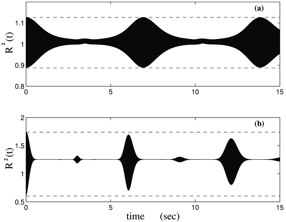
FIG. 1.: Collapses and revivals of oscillations of the mean square radius $R^{2}(t)$ of the condensate for $N=300$: a) the initial amplitude $2\rho_{1}=0.1$; b) the initial amplitude $2\rho_{1}=0.6$. Because of large time scale chosen, the rapid oscillations are seen as a black background. The dashed lines correspond to the envelope of the classical solutions

Note that the amplitude of the classical solution (see the dashed line in Fig.1) stays constant and equal to $2\rho_{1}$. In contrast, the collapses and the revivals of the amplitude of the oscillations of $R^{2}(t)$ determined quantum mechanically are clearly seen in qualitative accord with the analytical solution (9). We have approximated the initial collapse stage of the numerical solution by a gaussian fit to the envelope and found the characteristic collapse time $\tau_{c}$ as a function of the initial amplitude $2\rho_{1}$. The result for $1/\tau_{c}$ is represented in Fig.2. As can be seen, this graph is very close to the straight line predicted by Eq.(10). Its slope is $7.0s^{-1}$ while the analytical formula (10) gives $10s^{-1}$. These values yield the shortest dephasing time (corresponding to $\rho_{1}=1/2$ in Eqs.(9),(10)) as $\approx 0.1s$ which is comparable to the relaxation times ($\approx 150$ ms [8] and $\approx 250$ ms [9]) reported experimentally.

A direct confirmation of the proposed mechanism would be the experimental observation of the revivals. In this regard we note that the expected values of $\tau_{r}$ are of the order of seconds as given by the analytical estimates and the numerical solution (see Fig.1). This is comparable with the lifetime of the condensate in the traps [1, 2, 3, 4]. Furthermore, the normal component which introduces irreversible dissipation would inhibit the revivals unless its concentration is strongly suppressed. We will discuss this point in greater detail in future work. An estimate of the degree of the required suppression can be obtained from the following considerations. The rate $1/\tau_{n}$ of the thermal dissipation should be proportional to the relative amount $p$ of the normal component in the trap. In other words $1/\tau_{n}=p/\tau_{0}$, where $\tau_{0}$ is the relaxation time above $T_{BEC}$ when all particles constitute the normal component ($p=1$). This time is about $\tau_{0}\approx 20$ms [8, 9]. Consequently, in order to observe the revival of the oscillations at times $t>\tau_{r}$, the temperature should be reduced so that the condition $\tau_{n}>>\tau_{r}$ or $p<<\tau_{0}/\tau_{r}\sim 10^{-3}$ holds.

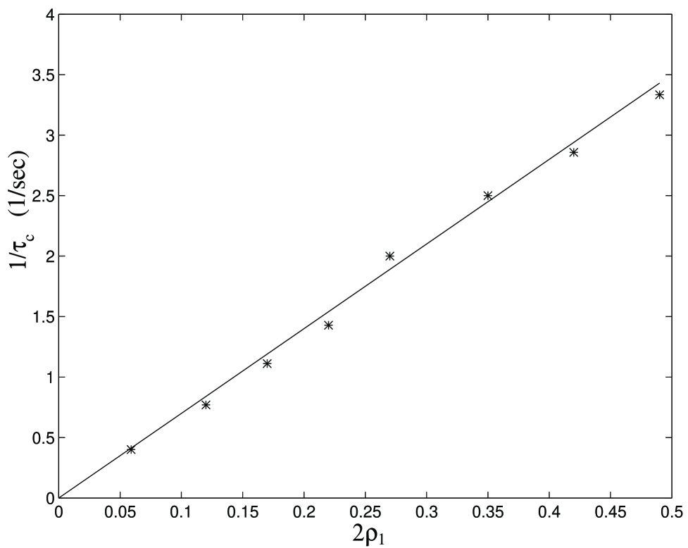
FIG. 2.: The rate of the first collapse as a function of the initial amplitude $2\rho_{1}$ for $N=300$. The line is a guide for eyes.

An indirect indication would be the observation of the relaxation of the oscillations described by the gaussian dependence, with the relaxation rate proportional to the initial response amplitude (for the small amplitudes) as predicted by Eq.(10) and Fig.2. Furthermore, Eq.(10) predicts a specific dependence on $N$. Let us focus on this fact in detail. The coefficient $g_{1}$ in Eq.(10) is given by the effective volume $V$ occupied by the condensate as $g_{1}\sim a/V\sim a\rho/N$. For small $N$ the density $\rho\sim N$ yielding $1/\tau_{c}\sim\sqrt{N}$ in Eq.(10). For $N>200-500$ the volume $V$ expands as a function of $N$ due to the inter particle interaction [11]. Accordingly, the dependence of $1/\tau_{c}$ should deviate from $\sim\sqrt{N}$. If $\rho$ were independent on $N$, one would have obtained $1/\tau_{c}\sim\rho/\sqrt{N}\to 0$ which implies no dephasing for large $N$. In the approximation we employed contributions of the higher order terms in $\rho$ to $g_{1}$ were neglected. Therefore, even though $\rho$ grows with $N$ ($\rho\sim N^{2/5}$ [11] for large $N$), the dephasing rate, as given by Eq.(10), is expected to vanish as a slow function of $N$ ($1/\tau_{c}\sim N^{-1/10}$) for large $N$. The higher order terms in $\rho$ contributing to the dephasing rate could change this conclusion. In future work we will analyze the limit of large $N$ by means of finding a better choice for the single particle state $\psi_{1}$ for large $N$ using the Bogolubov approach.

In conclusion, we have proposed a mechanism of interaction induced dephasing of the collective excitations in the atomic traps. The calculated collapse time is comparable to the observed relaxation times for the collective modes. Two main features – gaussian relaxation with the time constant depending linearly on the initial amplitude of the oscillations and depending on the total number of atoms – if observed experimentally, could verify this mechanism. If the temperature could be reduced much below $T_{BEC}$, the revivals of the collective oscillations could be seen on times of several seconds.

We are grateful to Yuri Kagan for very useful discussions. This research was supported by grants from The City University of New York PSC-CUNY Research Award Program.

REFERENCES

- [1] M.H. Anderson, J.R. Ensher, M.R. Matthews, C.E. Wieman, and E.A. Cornell, Science 269, 198 (1995).
- [2] C.C. Bradley, C.A. Sackett, J.J. Tollett, and R.G. Hulet, Phys. Rev. Lett.75, 1687 (1995).
- [3] K.B. Davis, M.-O. Mewes, M.R. Andrews, N.J. van Druten, D.S. Durfee, D.M. Kurn, and W. Ketterle, Phys. Rev. Lett. 75, 3969 (1995).
- [4] M.-O. Mewes, M.R. Andrews, N.J. van Druten, D.M. Kurn, D.S. Durfee, and W. Ketterle, Phys. Rev. Lett. 77, 416 (1996).
- [5] S. Stringari, Phys. Rev. Lett. 77, 2360 (1996).
- [6] M. Edwards, P.A. Ruprecht, K. Burnett, R.J. Dodd and C.W. Clark, Phys. Rev. Lett. 77, 1671 (1996).
- [7] Yu.Kagan, E. L. Surkov, and G. V. Shlyapnikov, Phys. Rev. A 54, R1753(1996).
- [8] D.S. Jin, J.R. Ensher, M.R. Matthews, C. E. Wieman, and E.A. Cornell, Phys. Rev. Lett. 77, 420 (1996).
- [9] M.-O. Mewes, M.R. Andrews, N.J. van Druten, D.M. Kurn, D.S. Durfee, C.G. Townsend, and W. Ketterle, Phys. Rev. Lett. 77, 988 (1996).
- [10] E.M. Lifshitz and L.P. Pitaevskii, Statistical Physics, Part 2 (Pergamon Press, Oxford, 1980).
- [11] G. Baym and C.J. Pethick, Phys. Rev. Lett. 76, 6 (1996).
- [12] N.B. Narozhny, J.J. Sanchez-Mondragon, and J.H. Eberly, Phys.Rev. A 23, 236 (1981).
- [13] M. Brune, F. Schmidt-Kaler, A. Maali, J. Dreyer, E. Hagley, J.M. Raimond, and S. Haroche, Phys. Rev. Lett. 76, 1800 (1996); D.M. Meekhof, C. Monroe, B.E. King, W.M. Itano, and D.J. Wineland, Phys. Rev. Lett. 76, 1796 (1996).
- [14] E. M. Wright, D. F. Walls, J. C. Garrison, Phys. Rev. Lett. 77, 2158(1996).
- [15] M. Lewenstein and L. You, Phys. Rev. Lett 77, 3489 (1996).
- [16] J. Ruostekoski and D. F. Walls, unpublished (cond-mat/9611074 preprint)
- [17] C.Leichtle, I. Sh. Averbukh, and W.P. Schleich, Phys.Rev.Lett. 77, 3999 (1996).
- [18] J. Blaizot and G. Ripka,Quantum Theory of Finite System. The MIT Press. Cambridge. 1986.
- [19] Furthermore, a frequency of the mode should not be restricted by the symmetry requirements which rely essentially on the infinite number of the one particle levels in the trapping potential as is the case for the center of mass motion and for the breathing modes in 2D [20]
- [20] L.P. Pitaevskii, and A. Rosch, unpublished ( preprint cond-mat/9608135 v2).