Nonequilibrium transport and population inversion in double quantum dot systems

Abstract

We present a microscopic theory for both equilibrium and nonequilibrium transport properties of coupled double quantum dots (DQD). A general formula for current tunneling through the DQD is derived by the nonequilibrium Green’s function method. Using a Hartree-Fock approach, effects of multi-level coupling and nonequilibrium electron distributions in resonant tunneling are considered. We find that the peak in the resonant tunneling current through two symmetric dots will split only when the inter-dot coupling is stronger than dot-lead coupling. We predict that population inversion can be achieved in one dot in the nonequilibrium regime.

Coupled quantum dot systems have received much attention recently [1, 2, 3, 4, 5, 6, 7, 8, 9]. Resonant tunneling through zero dimensional (0D) states of coupled quantum dots has been studied experimentally by several groups in both equilibrium ($|\mu_{L}-\mu_{R}|\ll k_{B}T$) and nonequilibrium ($|\mu_{L}-\mu_{R}|\gg k_{B}T$) regimes [1, 2, 3] (where $\mu_{L}$ and $\mu_{R}$ are chemical potentials of leads externally attached to the quantum dots from left and right, respectively). The Coulomb blockade theory (CBT) was used to study the equilibrium properties of electronic tunneling in a double quantum dot (DQD) system [4], and more recently[8, 9], has been extended to explain the tunneling current peak splitting observed in the experiment of Waugh et al[3].

Most previous theoretical studies on DQD systems [4, 5, 6, 8, 9] concentrated on the equilibrium properties. Interesting properties in the nonequilibrium regimes [2], where each dot can have different thermal nonequilibrium states driven by the two leads, have received much less attention. In this paper, we use a microscopic tunneling model to study the electronic transport through DQD systems based on the nonequilibrium Green’s function (NGF) method. Using the NGF method, the resonant tunneling current can then be derived exactly in both equilibrium and nonequilibrium regimes for tunneling through an interacting quantum dot [10] and non-interacting multi-quantum dots [11]. Here we give a general expression for the current for tunneling through interacting multi-level double quantum dot systems. The general current we derived can be used to obtain the well-known current equations in the equilibrium regime. In the nonequilibrium regime, it is usually difficult to satisfy detailed current balance between different dots and leads in various approximations [12], except in the case that the contribution to the imaginary self-energy is only from the lead-dot coupling. In this case, the current equation is much simplified and can be written in a compact form.

In this paper, we study resonant tunnelings through double quantum dots, each of them having more than 50 electrons. In these systems, only the quasi-particle states are relevant to the resonant tunneling. The spectrum of quasi-particle states near the Fermi surface will not change significantly with changing the electron number from $N$ to $N+1$ except for a slight energy level shift mainly due to the “charging effect”. This has been confirmed for quantum dot systems with $N>30$ by microscopic calculations [20]. In general, various scattering contributions to the imaginary self-energy (scattering-in scattering-out processes) can be discussed phenomenologically using our current equation below, which is useful for interpretation of experiments. We will use the general current equation derived here to discuss experimental results performed in the nonequilibrium regime [2]; some of our explanations are different from previous ones[2]. In particular, we will see that the study of nonequilibrium electron distributions in the quantum dots are crucial to understand nonequilibrium experiments [2]. If the couplings of lead-dot and dot-dot are $\Gamma$ and $|t|$, respectively, we predict that in symmetric equilibrium experiments [3] a peak of the resonant tunneling current will split only when $|t|>\Gamma/2$ with a splitting magnitude $2(|t|^{2}-\Gamma^{2}/4)^{1/2}$.

Particularly, we predict that a population inversion can be achieved in one of the two quantum dots when the tunneling between the two dots is in resonance. This population inversion should be easily realized under conditions such as the low temperature experiments of Ref.[2, 3]. At high temperatures, the population inversion critically depends on electron-phonon (e-p) or electron-electron (e-e) scattering induced relaxation times. This population inversion is similar to that in quantum cascade lasers (QCL) [15] except that the former co-exists with resonant tunneling and the tunneling is not photon-assisted. Thus population inversion can be achieved in the double quantum wells under similar conditions as for QCL.

The structure of this paper is as follows: in section I we discuss the model and derive the general current equations; in section II we discuss various approximations and the simplified current equations; in section III we discuss the non-equilibrium distribution of electrons in a double quantum dot system and the possibility of population inversion; in section IV, we discuss two recent experiments; and we conclude in section V.

I Model and Current Equations

We model the coupled DQD system with two attached leads by the Hamiltonian [13] $H=H_{0}+H_{t}+H_{I}$, with

$$H_{0} = \psi_{L}^{\dagger}{\bf E}^{L}\psi_{L}+\psi_{R}^{\dagger}{\bf E}^{R}\psi_{R}+\sum_{i=1,2}\psi_{i}^{\dagger}{\bf E}^{(i)}\psi_{i}$$ (1)

$$H_{t} = \psi_{L}^{\dagger}{\bf V_{L,1}}\psi_{1}+\psi_{R}^{\dagger}{\bf V_{R,2}}\psi_{2}+\psi_{1}^{\dagger}{\bf t_{12}}\psi_{2}+h.c.,$$ (2)

where the subscripts ($L$, $R$) represent the left- and right-lead, and ${i}$ sums over the two dots. In Hartree-Fock (HF) representation, $\psi^{\dagger}_{\alpha\in\{L,R\}}=(a^{\dagger}_{k_{1}\alpha},a^{\dagger}_{k_{2}\alpha},\cdots,a^{\dagger}_{k_{N_{\alpha}}\alpha})$, $\psi^{\dagger}_{i\in\{1,2\}}=(c^{\dagger}_{i,1},c^{\dagger}_{i,2},\cdots,c^{\dagger}_{i,n_{i}})$. Here {$k_{1},\cdots k_{N_{\alpha}}$} and $\{1,2,\cdots n_{i}\}$ are labels of states in the lead and dot, $N_{\alpha}$ and $n_{i}$ are the numbers of total states in the lead-$\alpha$ and dot-$i$, respectively. The ${\bf E}^{i}$’s are diagonal matrices whose elements are calculated in the HFA. $H_{t}$ is a tunneling Hamiltonian. ${\bf V}_{\alpha,i}\equiv[V^{\alpha,i}_{k_{m},l}]$ is the ($N_{\alpha}\times n_{i}$) hopping integral matrix; the matrix element $V^{\alpha,i}_{k_{m},l}$ is the hopping integral from state $k_{m}$ in lead-$\alpha$ to state-$l$ in dot-$i$. ${\bf t}_{12}\equiv[t^{1,2}_{l,m}]$ is a ($n_{1}\times n_{2}$) matrix, and the matrix element $t^{1,2}_{l,m}$ is the hopping integral from state-$l$ in dot-$1$ to state-$m$ in dot-$2$. $H_{I}$ describes residual interactions such as electron-phonon (e-p) scattering, disorder scattering, and e-e correlations.

Since the system under investigation is in non-thermal equilibrium in the nonlinear region (with finite bias voltage), The natural technique to use is that of non-equilibrium Green functions [16, 17, 18] (NGF). The NGF in the DQD in matrix form is defined by:

$${\bf G}_{i,j}(\tau,\tau^{\prime})=-i\left\langle{\cal T}_{C}\left\{\psi_{i}(\tau)\psi^{\dagger}_{j}(\tau^{\prime})\right\}\right\rangle,$$ (3)

where ${\cal T}_{C}$ is the chronological time-ordering operator on the contour $C$ of the closed time path, and $\tau\equiv(\beta,t)$ with $\beta=\pm$ in the plus (minus) branch of the contour $C$. We choose the bases as HF states, so the evolution of $\psi_{i}$ is governed by $H_{t}$ and $H_{I}$. Similarly, we define the GF for the two leads ${\bf G}_{L}$ and ${\bf G}_{R}$, and the “off-diagonal” NGF ${\bf G}_{L,1}$ and ${\bf G}_{R,2}$, etc. The four combinations of the time branches $(\pm,\pm)$ give four linearly dependent component NGFs. Here we have used the notation that ${\bf G}_{\gamma,\delta}$ without superscript index means a ($2\times 2$) matrix of ${\bf G}_{\gamma,\delta}^{\pm\pm}$ with superscripts. After a rotation in the ($2\times 2$) space, we can obtain three independent components of the NGF, i.e., ${\bf G}^{r,a,+-}_{ij}$ (retarded, advanced and statistical component carrying information of nonequilibrium distributions). Another frequently used (Keldysh) statistical component of NGF instead of ${\bf G}^{+-}$ is ${\bf G}^{K}=2{\bf G}^{+-}+{\bf G}^{r}-{\bf G}^{a}$. Each of the three components is itself a ($n_{i}\times n_{j}$) matrix, where $n_{i}$ is the number of total states in dot-$i$ or lead-$i$. (Note that we have used the notation $n_{i}$ for the leads instead of $N_{\alpha}$, this is only for the convenience of description here). The matrix elements of these $n_{i}\times n_{j}$ NGF matrices are just the scalar NGF, e.g. $[G_{1,2}^{r}]_{l,m}(t,t^{\prime})=-i\Theta(t,t^{\prime})\langle\{c^{\phantom{\dagger}}_{l,1}(t),c^{\dagger}_{m,2}(t^{\prime})\}\rangle$.

Since the leads are open systems, we can treat them as two equilibrium Fermi seas of non-interacting quasi-particles with different chemical potentials. The degrees-of-freedom of the leads can be integrated out and the self-energies (in matrix form) of the two quantum dots due to the tunneling between the leads and dots become [11]: ${\bf\Sigma}^{0}_{1}(\omega)={\sigma}_{x}{\bf V_{L}}^{\dagger}{\bf G}_{L}{\bf V_{L}}{\sigma}_{x}$; ${\bf\Sigma}^{0}_{2}(\omega)={\sigma}_{x}{\bf V_{R}}^{\dagger}{\bf G}_{R}{\bf V_{R}}{\sigma}_{x}$, where $\sigma_{x}$ is the Pauli matrix operating only in the ($2\times 2$) Keldysh space [17]. Defining $i{\bf\Gamma}_{j}=({\bf\Sigma}^{0}_{j})^{r}-({\bf\Sigma}^{0}_{j})^{a}$, it is easy to see that: $({\bf\Sigma}^{0}_{1})^{+-}(\omega)=if_{L}(\omega){\bf\Gamma}_{1}(\omega)$ and $({\bf\Sigma}^{0}_{2})^{+-}(\omega)=if_{R}(\omega){\bf\Gamma}_{2}(\omega)$, with $f_{L}(\omega)$ and $f_{R}(\omega)$ the Fermi-Dirac distribution functions of the left and right leads, respectively. Physically, the diagonal matrix element $[\Gamma_{i}]_{l,l}$ of ${\bf\Gamma}_{i}$ is the level broadening of state-$l$ in dot-$i$ due to the tunneling to all the states in the neighboring lead.

The current equations can be derived formally using the Dyson equations. In our system, the Dyson equations (in Keldysh space) [17] can be written as:

$${\bf g}_{i}^{-1}{\bf G}_{ij} = {\bf\delta}_{ij}+{\bf\Sigma}_{ij}{\bf G}_{ij}+{\sigma}_{x}{\bf t}_{12}{\bf G}_{\bar{\imath}j},$$ (4)

where ${\bf g}_{i,j}\equiv{\bf g}_{i}\delta_{i,j}$ is the bare GF for $H_{0}$, $\bar{\imath}\in\{\bar{1}\equiv 2,\bar{2}\equiv 1\}$. To take into account the self-energy parts from the e-e correlations and e-p scattering $H_{I}$, $\mathchoice{{\hbox{\boldmath$\displaystyle\sigma$}}}{{\hbox{\boldmath$\textstyle\sigma$}}}{{\hbox{\boldmath$\scriptstyle\sigma$}}}{{\hbox{\boldmath$\scriptscriptstyle\sigma$}}}_{ij}$, we obtain the self-energies ${\bf\Sigma}_{ij}={\bf\Sigma}_{i}^{0}+\mathchoice{{\hbox{\boldmath$\displaystyle\sigma$}}}{{\hbox{\boldmath$\textstyle\sigma$}}}{{\hbox{\boldmath$\scriptstyle\sigma$}}}{{\hbox{\boldmath$\scriptscriptstyle\sigma$}}}_{ij}$. If there is no coupling between $\psi_{1}$ and $\psi_{2}$ other than tunneling, then $\mathchoice{{\hbox{\boldmath$\displaystyle\sigma$}}}{{\hbox{\boldmath$\textstyle\sigma$}}}{{\hbox{\boldmath$\scriptstyle\sigma$}}}{{\hbox{\boldmath$\scriptscriptstyle\sigma$}}}_{12}=\mathchoice{{\hbox{\boldmath$\displaystyle\sigma$}}}{{\hbox{\boldmath$\textstyle\sigma$}}}{{\hbox{\boldmath$\scriptstyle\sigma$}}}{{\hbox{\boldmath$\scriptscriptstyle\sigma$}}}_{11}$ and $\mathchoice{{\hbox{\boldmath$\displaystyle\sigma$}}}{{\hbox{\boldmath$\textstyle\sigma$}}}{{\hbox{\boldmath$\scriptstyle\sigma$}}}{{\hbox{\boldmath$\scriptscriptstyle\sigma$}}}_{21}=\mathchoice{{\hbox{\boldmath$\displaystyle\sigma$}}}{{\hbox{\boldmath$\textstyle\sigma$}}}{{\hbox{\boldmath$\scriptstyle\sigma$}}}{{\hbox{\boldmath$\scriptscriptstyle\sigma$}}}_{22}$.

The Dyson equations (4) can be solved easily: ${\bf G}_{ii}^{r,a}=[({\bf g}_{i}^{r,a})^{-1}-{\bf\tilde{\Sigma}}^{r,a}_{i}]^{-1}$, ${\bf G}_{ii}^{+-}={\bf G}_{ii}^{r}{\bf\tilde{\Sigma}}^{+-}_{i}{\bf G}_{ii}^{a}$, where we have used the total self-energy ${\bf\tilde{\Sigma}}_{i}={\bf\Sigma}_{ii}+{\bf\delta\Sigma}_{i}$ with

$${\bf\delta\Sigma}_{i} = {\sigma}_{x}{\bf t}_{12}\left[{\bf g}_{i}^{-1}-{\bf\Sigma}_{i\bar{\imath}}\right]^{-1}{\bf t}_{12}^{\dagger}{\sigma}_{x}\equiv{\sigma}_{x}{\bf t}_{12}{\bf\tilde{g}}_{i}{\bf t}_{12}^{\dagger}{\sigma}_{x}.$$ (5)

Here we have used five different self-energies. Their physical meaning is following: as described above, ${\bf\Sigma}^{0}_{i}$ is the self-energy due to tunneling to the neighboring lead; $\mathchoice{{\hbox{\boldmath$\displaystyle\sigma$}}}{{\hbox{\boldmath$\textstyle\sigma$}}}{{\hbox{\boldmath$\scriptstyle\sigma$}}}{{\hbox{\boldmath$\scriptscriptstyle\sigma$}}}_{ij}$ is the self-energy due to interactions $H_{I}$ without tunneling between quantum dots; ${\bf\delta\Sigma}_{i}$ is the self-energy due to tunneling to another dot (Note this self-energy is calculated using the renormalized GF ${\bf\tilde{g}}_{i}$); finally, ${\bf\tilde{\Sigma}}_{i}$ is the total self-energy.

From the Dyson equations, the current can easily be calculated at different dots:

$$J^{(\alpha,j)} = (-1)^{j+1}{ie\over h}\int d\omega Tr\{\left[({\bf\Sigma}^{0}_{j})^{r}-({\bf\Sigma}^{0}_{j})^{a}\right]{\bf G}_{jj}^{+-}$$ (7)

$$- ({\bf\Sigma}^{0}_{j})^{+-}\left[{\bf G}_{jj}^{r}-{\bf G}_{jj}^{a}\right]\}$$ (8)

$$J^{(j)} = (-1)^{j}{ie\over h}\int d\omega Tr\{\left[({\bf\delta\Sigma}_{j})^{r}-({\bf\delta\Sigma}_{j})^{a}\right]{\bf G}_{jj}^{+-}$$ (9)

$$- ({\bf\delta\Sigma}_{j})^{+-}\left[{\bf G}_{jj}^{r}-{\bf G}_{jj}^{a}\right]\},$$ (10)

where the superscripts $(\alpha,j)\in\{(L,1),(R,2)\}$ denotes the current tunneling from the lead to the dot-$i$, and $(j)$ is the inter-dot current calculated at dot-$j$.

II Simplified Current Equations: Approximations

In general, the introduction of $\mathchoice{{\hbox{\boldmath$\displaystyle\sigma$}}}{{\hbox{\boldmath$\textstyle\sigma$}}}{{\hbox{\boldmath$\scriptstyle\sigma$}}}{{\hbox{\boldmath$\scriptscriptstyle\sigma$}}}_{ij}$ makes the current in Eq.(I) non-conserved [12]. To obtain a current obeying detailed balance, current-conserving approximations for $\textstyle\sigma$ are required. However, since we adopt HFA here, when $H_{I}$ is neglected then the current in Eq.(I) is automatically conserved [11]. The current is now written in a simpler form:

$$J = {e\over h}\int d\omega(f^{FD}_{L}-f^{FD}_{R})T_{r}\left[{\bf G}_{22}^{a}{\bf\Gamma}_{1}{\bf G}_{22}^{r}{\bf t}_{12}{\bf\tilde{g}}^{r}_{1}{\bf\Gamma}_{2}{\bf\tilde{g}}^{a}_{1}{\bf t}_{12}^{\dagger}\right],$$ (11)

where $f^{FD}_{L,R}$ is the Fermi-Dirac distribution function and ${\bf\tilde{g}}_{i}$ is defined in Eq.(5). Recall that ${\bf t}_{12}{\bf\tilde{g}}^{r}_{1}{\bf\Gamma}_{2}{\bf\tilde{g}}^{a}_{1}{\bf t}_{12}^{\dagger}$ is just the imaginary part of self-energy ${\bf\delta\Sigma}_{i}$ due to tunneling between quantum dots. The current equation (11) is very similar to that for a single dot system, i.e. replace ${\bf\Gamma}_{\alpha}$ due to tunneling to the lead by ${\bf\Gamma}_{ij}=(\delta{\bf\Sigma}_{j})^{r}-(\delta{\bf\Sigma}_{j})^{a}$ due to tunneling from dot-$i$ to another dot-$j$.

The electron-electron (e-e) and electron-phonon (e-p) interactions have two kinds of effects: renormalizing ${\bf E}^{(i)}$ due to $\Re\mathchoice{{\hbox{\boldmath$\displaystyle\sigma$}}}{{\hbox{\boldmath$\textstyle\sigma$}}}{{\hbox{\boldmath$\scriptstyle\sigma$}}}{{\hbox{\boldmath$\scriptscriptstyle\sigma$}}}^{r,a}$ and changing the distribution of electrons due to $\mathchoice{{\hbox{\boldmath$\displaystyle\sigma$}}}{{\hbox{\boldmath$\textstyle\sigma$}}}{{\hbox{\boldmath$\scriptstyle\sigma$}}}{{\hbox{\boldmath$\scriptscriptstyle\sigma$}}}^{K}$ (and $\Im\mathchoice{{\hbox{\boldmath$\displaystyle\sigma$}}}{{\hbox{\boldmath$\textstyle\sigma$}}}{{\hbox{\boldmath$\scriptstyle\sigma$}}}{{\hbox{\boldmath$\scriptscriptstyle\sigma$}}}^{r,a}$). In the former effect, we simply renormalize [19] ${\bf E}^{(i)}$, so the current equation is the same as Eq.(11). After we include the higher order (than HFA) energy shift, Eq.(11) contains rich correlation effects. One example is for the two-impurity model in the Hartree approximation studied by Niu et al [7]. One might attempt to calculate the interacting NGFs using higher order (than Hartree approximation) truncation of the EOM and then calculate tunneling currents using Eq.(11). This is questionable for double dot systems except when the truncated EOM is in the form of a Dyson equation. Otherwise, one needs to re-derive the current equation using the truncated EOM. For large quantum dots with more than $40$ electrons, only the quasiparticle states near the Fermi surface are relevant to the resonant tunneling. The spectral functions of these quasiparticle states do not change significantly with adding/subtracting a couple of electrons in the dots except for a slight energy level shift due to the “charging effects”. This has been confirmed by microscopic calculations by Wang, Zhang, and Bishop [20], who also found that the many-electron energy levels are approximately equally spaced for quantum dots with more than 30 electrons. Thus for quantum dots with a large occupation numbers, the energy shift due to e-e interactions can be treated phenomenologically (see Sec.IV) and the level spacing can be extracted from experiments. The scattering-in/out effect due to $\mathchoice{{\hbox{\boldmath$\displaystyle\sigma$}}}{{\hbox{\boldmath$\textstyle\sigma$}}}{{\hbox{\boldmath$\scriptstyle\sigma$}}}{{\hbox{\boldmath$\scriptscriptstyle\sigma$}}}^{K}$ is difficult to treat correctly in various approaches due to the detailed current balance problem mentioned above. However, qualitative effects can still be obtained after simplifying Eq.(I) appropriate to different conditions, in a similar fashion to our discussions of nonequilibrium distributions below.

Up to now, our equations are general for multi-level dots. To study a specific system, we need to know the matrix elements $[{\bf t}_{12}]_{l_{i}l_{j}}$ (hopping) and $\left[{\bf\Gamma}_{i}\right]_{l_{i}l_{j}}$. Let us first examine the relevance of various matrix elements. The elements $\left[{\bf\Gamma}_{i}\right]_{l_{i}l_{j}}$ for $l_{i}\neq l_{j}$ are due to tunneling from different levels $l_{i}$ and $l_{j}$ to the same state in the lead. These are usually not small compared to the diagonal ones, and they describe the mixing of levels in the dots due to tunneling to the leads. If we assume the energy of the states in the tunneling window (i.e. $\mu_{1}<E_{i}<\mu_{2}$) is much smaller than the barrier height between leads and dots, then $\left[{\bf\Gamma}_{i}\right]_{l_{i}l_{j}}=\Gamma_{i}$. The matrix elements $[{\bf t}_{12}]_{l_{i}l_{j}}$ describe wavefunction overlaps of different levels between two quantum dots. The value of these matrix elements are different but roughly of the same magnitude if their energies are comparable. Similarly, if we assume the energy of the states in the tunneling window (i.e. $\mu_{1}<E_{i}<\mu_{2}$) is much smaller than the barrier height between two dots, then we can use the following assumption $[{\bf t}_{12}]_{l_{i}l_{j}}=t$ (thick-shell model [9]). Using the assumption $\left[{\bf\Gamma}_{i}\right]_{l_{i}l_{j}}=\Gamma_{i}$,

$$\left[{\bf\tilde{g}}^{r,a}_{\alpha}\right]_{ij}=\cases{{1\over w_{i}^{r,a}}\left(1+{1\over w_{i}^{r,a}}{(\Sigma^{0}_{\alpha})^{r,a}\over 1-(\Sigma^{0}_{\alpha})^{r,a}\sum_{k}{1\over w_{k}^{r,a}}}\right)&$i=j$;\cr\cr{(\Sigma^{0}_{\alpha})^{r,a}\over w_{i}^{r,a}w_{j}^{r,a}\left(1-(\Sigma^{0}_{\alpha})^{r,a}\sum_{k}{1\over w_{k}^{r,a}}\right)}&$i\neq j$.\cr}$$ (12)

where $w_{i}^{r,a}=[({\bf g}_{\alpha}^{r,a})^{-1}]_{ii}$.

In the experiments [2, 3], $\Gamma_{i}$, $|t|\ll\Delta E$ (spacing between energy levels in the dots). Using Eq.(12), it is easy to show that near the resonance $\omega\sim\epsilon_{l_{0}}$: for $l_{i}=l_{0}$, $\left[{\bf\tilde{g}}^{r}_{1}\right]_{l_{i}l_{i}}\sim 1/\Gamma_{1}$; for $l_{i}\neq l_{0}$; $\left[{\bf\tilde{g}}^{r}_{1}\right]_{l_{i}l_{i}}\sim 1/[(l_{i}-l_{0})\Delta E]$; for $l_{i}\neq l_{j}\neq l_{0}$, $\left[{\bf\tilde{g}}^{r}_{1}\right]_{l_{i}l_{j}}\sim(\omega-\epsilon_{l_{0}})/[(l_{i}-l_{0})(l_{j}-l_{0})(\Delta E)^{2}]$; for $l_{i}=l_{0}$, $l_{j}\neq l_{0}$, $\left[{\bf\tilde{g}}^{r}_{1}\right]_{l_{i}l_{j}}\sim 1/[(l_{j}-l_{0})\Delta E]$. The properties of the $[{\bf G}_{ij}^{r}]_{l_{i}l_{j}}$ are similar. Thus, at $\Gamma_{i},|t|\ll\Delta E$, only the tunnelings between levels close to each other are important.

For the resonant peak structure, we can simplify Eq.(11) near resonance, $\mu_{L}>\epsilon^{(1)}_{l_{1}}\sim\epsilon^{(2)}_{l_{2}}>\mu_{R}$, by taking into account only the resonance level contribution:

$$J \simeq \int d\omega(f_{L}-f_{R}){\Gamma_{2}\Gamma_{12}\over(\omega-{\epsilon}^{(2)}_{l_{2}}-\delta\epsilon^{(2)})^{2}+(\Gamma_{2}/2+\Gamma_{12}/2)^{2}}$$ (13)

$$\simeq {e\over h}\int d\omega{f_{L}-f_{R}\over(\omega-\epsilon^{(1)}_{l_{1}})^{2}+(\Gamma_{1}/2)^{2}}{\Gamma_{2}\Gamma_{1}|t|^{2}\over(\omega-{\epsilon}^{(2)}_{l_{2}}-{|t|^{2}(\omega-{\epsilon}^{(1)}_{l_{1}})\over(\omega-{\epsilon}^{(1)}_{l_{1}})^{2}+(\Gamma_{1}/2)^{2}})^{2}+({\Gamma_{2}\over 2}+{\Gamma_{1}\over 2}{|t|^{2}\over(\omega-{\epsilon}^{(1)}_{l_{1}})^{2}+(\Gamma_{1}/2)^{2}})^{2}},$$ (14)

where we have used definitions $i{\bf\Gamma}_{12}=(\delta{\bf\Sigma}_{2})^{r}-(\delta{\bf\Sigma}_{2})^{a}$ and $\delta\epsilon^{(2)}=\Re(\delta{\bf\Sigma}_{2})^{r}$. Near resonance, $\mu_{L}>\epsilon^{(1)}_{l_{1}}\sim\epsilon^{(2)}_{l_{2}}>\mu_{R}$, $\Gamma_{12}=\Gamma_{1}{|t|^{2}\over(\omega-\epsilon^{(1)}_{l_{1}})^{2}+(\Gamma_{1}/2)^{2}}$; $\delta\epsilon^{(2)}={|t|^{2}(\omega-{\epsilon}^{(1)}_{l_{1}})\over(\omega-{\epsilon}^{(1)}_{l_{1}})^{2}+(\Gamma_{1}/2)^{2}}$.

III Nonequilibrium Distributions in the Dots and Population Inversion

Before discussing the resonant current, let us first consider the nonequilibrium distributions of electrons in the two dots. The distribution at each level $l_{i}$ of dot $i$ is given by

$$F^{i}_{l_{i}}(\epsilon) = [G^{+-}_{ii}]_{l_{i}l_{i}}(\epsilon)/([G^{r}_{ii}]_{l_{i}l_{i}}-[G^{a}_{ii}]_{l_{i}l_{i}})$$ (15)

$$\frac{HFA}{i=2,l_{i}=l_{2}} \rightarrow{f^{FD}_{R}+f^{FD}_{L}\lambda(\epsilon^{(2)}_{l_{2}})\Gamma_{1}/\Gamma_{2}\over 1+\lambda(\epsilon^{(2)}_{l_{2}})\Gamma_{1}/\Gamma_{2}}$$ (16)

$$\frac{HFA}{i=1,l_{i}=l_{1}} \rightarrow{f^{FD}_{L}+f^{FD}_{R}\lambda(\epsilon^{(1)}_{l_{1}})\Gamma_{2}/\Gamma_{1}\over 1+\lambda(\epsilon^{(1)}_{l_{1}})\Gamma_{2}/\Gamma_{1}}$$ (17)

with $\lambda(\epsilon^{(i)}_{l_{i}})\Gamma_{\bar{\imath}}=\Gamma_{\bar{\imath}}|t|^{2}\sum_{klm}\left[{\bf\tilde{g}}^{r}_{\bar{\imath}}\right]_{kl}\left[{\bf\tilde{g}}^{a}_{\bar{\imath}}\right]_{lm}$ the energy level broadening due to tunneling between dots. When the level $\epsilon^{(2)}_{l_{2}}<\mu_{R}$ ($\mu_{R}<\mu_{L}$ according to our convention), $f^{FD}_{L}(\epsilon^{(2)}_{l_{2}})=f^{FD}_{R}(\epsilon^{(2)}_{l_{2}})=1$, $F^{2}_{l_{2}}(\epsilon^{(2)}_{l_{2}})=1$, this level in the dot is occupied; when the level $\epsilon^{(2)}_{l_{2}}>\mu_{L}$, $f^{FD}_{L}(\epsilon^{(2)}_{l_{2}})=f^{FD}_{R}(\epsilon^{(2)}_{l_{2}})=0$, $F^{2}_{l_{2}}(\epsilon^{(2)}_{l_{2}})=0$, this level is empty. ¿From Eq.(11), the energy levels in these two cases do not contribute to the resonant tunneling. A more interesting case is for levels lying between $\mu_{R}$ and $\mu_{L}$, where $f^{FD}_{L}=1$ and $f^{FD}_{R}=0$, electrons are in nonequilibrium states, and $F^{2}_{l_{2}}\sim{\lambda_{2}\Gamma_{1}\over\Gamma_{2}+\lambda_{2}\Gamma_{1}}$ strongly depends on the energy spectrum in the first dot. Using the properties of $\left[{\bf\tilde{g}}^{r}_{1}\right]_{l_{i}l_{j}}$, when a level-$i_{u}$ of dot-2 is in resonance with a level in dot-1, $\lambda_{2}\sim|t|^{2}/(4\Gamma_{1}^{2})$, the occupation number of level-$i_{u}$ is $F^{2}_{i_{u}}\sim{|t|^{2}\over 4\Gamma_{1}\Gamma_{2}+|t|^{2}}$; when a level-$i_{d}$ of dot-2 is not in resonance with levels in dot-1, $\lambda_{2}\sim(|t|/\Delta E)^{2}\ll 1$, the occupation number of level-$i_{d}$ is given by $F^{2}_{i_{d}}\sim|t/\Delta E|^{2}\Gamma_{1}/\Gamma_{2}\ll\Gamma_{1}/\Gamma_{2}$.

There is a population inversion in the dot-2 ($|t|\sim\Gamma$) when $\epsilon^{(2)}_{i_{u}}>\epsilon^{(2)}_{i_{d}}$: the population inversion in dot-2 can be achieved due to the resonance of a higher level-$i_{u}$ (relative to an active level-$i_{d}$) in dot-2 with a level in dot-1. The nonequilibrium electron distribution in dot-1 is similar. When the level $\epsilon^{(1)}_{l_{1}}<\mu_{R}$, $F^{1}_{l_{1}}(\epsilon^{(1)}_{l_{2}})=1$, this level in the dot is occupied; when the level $\epsilon^{(1)}_{l_{1}}>\mu_{L}$, $F^{1}_{l_{1}}(\epsilon^{(1)}_{l_{1}})=0$, this level is empty. When $\mu_{R}<\epsilon^{(1)}_{l_{1}}<\mu_{L}$, $F^{1}_{l_{1}}\sim{\Gamma_{1}\over\Gamma_{1}+\lambda_{1}\Gamma_{2}}$. When this level is not in resonance with a level in dot-2, $\lambda_{1}\sim(|t|/\Delta E)^{2}\ll 1$, $F^{1}_{l_{1}}\sim 1$; otherwise, $\lambda_{1}\sim|t|^{2}/(4\Gamma_{2}^{2})$, $F^{1}_{l_{1}}\sim 1/(1+|t|^{2}/(4\Gamma_{1}\Gamma_{2}))$. Thus, with $|t|\ll\Gamma_{i}$, $F^{1}_{l_{1}}\sim 1$ when $\mu_{R}<\epsilon^{(1)}_{l_{1}}<\mu_{L}$.

This population inversion is similar to that in quantum cascade lasers for superlattices [15] and other proposals for double quantum wells [25]. However, the population inversions proposed previously for quantum wells are achieved without elastic resonant tunneling. For example, in the double quantum well systems [25], the upper level is attached to the lead with high chemical potential $\mu_{h}$ and with $E_{u}<\mu_{h}$, so the upper level is occupied; the lower level (either in the same well or in another well) is attached to the lead with lower chemical potential $\mu_{l}$ with $E_{l}>\mu_{l}$, thus it is empty. Since transverse momentum is conserved and can be neglected the quantized energy levels in the wells are mismatched, there is no elastic resonant tunneling, and the system is in quasi equilibrium with two chemical potentials $\mu_{h}$ and $\mu_{l}$. The electrons can only tunnel via emitting photons. In the population inversion we proposed above, the energy levels are not in quasi equilibrium with the leads. The population inversion is achieved through resonant tunneling. Comparing to the proposal in Ref.[25] for double quantum wells, we believe that our proposal is easier to realize practically.

In the above analysis, we have neglected the inelastic scattering effects due to e-e and e-p couplings. In real systems, the e-e and e-p scatterings have important effects on the nonequilibrium distribution of electrons in the dots. At high temperatures, the nonequilibrium distribution will be thermalized due to inelastic relaxation. Here we concentrate on low temperatures, when the dominant contribution to $\textstyle\sigma$ comes from higher order e-e correlations which will affect the NGF’s. Taking this fact into account, the $F$-function with a finite $\textstyle\sigma$ becomes:

$$F^{2}_{i}(\epsilon^{(2)}_{l_{2}})={\sigma_{22}^{+-}+\lambda(\epsilon^{(2)}_{l_{2}})\Gamma_{1}\over\Gamma_{2}+\gamma_{2}+\lambda(\epsilon^{(2)}_{l_{2}})\Gamma_{1}},$$ (18)

where $i\mathchoice{{\hbox{\boldmath$\displaystyle\gamma$}}}{{\hbox{\boldmath$\textstyle\gamma$}}}{{\hbox{\boldmath$\scriptstyle\gamma$}}}{{\hbox{\boldmath$\scriptscriptstyle\gamma$}}}_{j}=\mathchoice{{\hbox{\boldmath$\displaystyle\sigma$}}}{{\hbox{\boldmath$\textstyle\sigma$}}}{{\hbox{\boldmath$\scriptstyle\sigma$}}}{{\hbox{\boldmath$\scriptscriptstyle\sigma$}}}_{j}^{r}-\mathchoice{{\hbox{\boldmath$\displaystyle\sigma$}}}{{\hbox{\boldmath$\textstyle\sigma$}}}{{\hbox{\boldmath$\scriptstyle\sigma$}}}{{\hbox{\boldmath$\scriptscriptstyle\sigma$}}}_{j}^{a}$ with the assumption $[\mathchoice{{\hbox{\boldmath$\displaystyle\gamma$}}}{{\hbox{\boldmath$\textstyle\gamma$}}}{{\hbox{\boldmath$\scriptstyle\gamma$}}}{{\hbox{\boldmath$\scriptscriptstyle\gamma$}}}_{j}]_{l_{j}l^{\prime}_{j}}=\gamma_{2}$. Physically, $\gamma_{2}$ is just the average level broadening due to e-e scattering. $\sigma_{22}^{+-}$ is responsible for changing of the distribution functions. Note that $\sigma_{22}^{+-}\lesssim\gamma_{2}$. Here $\lambda(\epsilon^{(2)}_{l_{2}})$ has been changed due to the introduction of $\sigma$. So at resonance of level-$i_{u}$, $F^{2}_{i_{u}}\sim{{|t|^{2}\Gamma_{1}+4(\sigma_{22})_{i_{u},i_{u}}^{+-}(\Gamma_{1}+\gamma_{1})^{2}\over 4(\Gamma_{2}+\gamma_{2})(\Gamma_{1}+\gamma_{1})^{2}+|t|^{2}\Gamma_{1}}}$, while $F^{2}_{i_{d}}\sim(\sigma_{22})_{i_{d},i_{d}}^{+-}/(\Gamma_{2}+\gamma_{2})$. If $(\sigma_{22})_{i_{u},i_{u}}^{+-}\sim(\sigma_{22})_{i_{d},i_{d}}^{+-}$, it is easy to show that $F^{2}_{i_{u}}>F^{2}_{i_{d}}$. In the extreme case that $(\sigma_{22})_{i_{d},i_{d}}^{+-}\sim\gamma_{2}$ and $(\sigma_{22})_{i_{u},i_{u}}^{+-}\sim 0$, the population inversion survives when $|t|^{2}>{4\gamma_{2}(\Gamma_{2}+\gamma_{2})\over\Gamma_{1}\Gamma_{2}}(\Gamma_{1}+\gamma_{1})^{2}$. For the e-e scattering in the typical experiments $\gamma_{i}\lesssim\Gamma_{i}$ [20], so the population inversion can be achieved at $|t|\gg\Gamma$. Consequently, the e-e correlations reduce the magnitude of the resonant current but do not qualitatively change the resonance peak structure.

IV Nonequilibrium Currents and Peak Splittings

A Nonequilibrium Currents

In this section, we discuss the recent nonequilibrium experiments of Ref.[2] using the general equations derived above. In these experiments, $\Gamma_{i}$, $|t|\ll\Delta E$, so we can neglect the contributions of energy levels far from resonance (i.e. for experiment [2], we only need take into account 4 relevant levels). We use Eq.(11) to calculate the currents, which neglects the high order scattering-in(out) processes. This is a reasonable approximation for low temperature experiments of quantum dots with electron numbers on the order of 90 [20], as we discussed above.

The oscillations of the nonlinear resonant tunneling current vs. gate voltage in experiment [2] can be readily explained if we take into account the charging effect [13, 22] for the renormalized HF energy levels $\epsilon^{(1)}_{l_{1}}$ and $\epsilon^{(2)}_{l_{2}}$ [see Fig.1]. In Fig.2 we plot the conductance of the current tunneling through the DQD vs. the gate voltage $V_{g1}$ on dot-1 using a constant bias voltage of $280\mu V$. (Only one group of the peaks is shown). The current is calculated using Eq.(11) for $|t|=0.2\mu eV$; $\Gamma_{1}=\Gamma_{2}=4.0\mu eV$, 10.0$\mu eV$; the level spacing in dot-1 and dot-2 as $\Delta E^{(1)}=150\mu eV$ and $\Delta E^{(2)}=230\mu eV$, respectively.

Our assignment of the peaks in Fig.(2) is the same as that in Ref.[2]. We assume in Fig.(2) that the spectrum in dot-2 is fixed while varying $V_{g1}$. Using the energy level spacings given in Ref.[2], the spacing between the first and second peaks is $\sim 80\mu eV$, and the spacing between the second and third peaks is $\sim 150\mu eV$. However, in the experimental I-V curves, the first spacing is larger than the second one. One possible reason is that the level spacing is not regular, which is suggested in Ref.[2]. Note that the gate voltage scale for these spacings are $\sim 900\mu V$ and $2500\mu V$ respectively. In Ref.[2] they are converted to energy scales as $70\mu eV$ and $200\mu eV$. Then the level spacing between level-2 and level-3 in dot-1 is barely half of the average level spacing. Another possibility is that this discrepancy can be due to the charging effect. As discussed in Sec.III, without resonance between the two dots, the “active” levels in dot-1 are filled and the “active” levels in dot-2 are empty; with resonance, the resonance level in dot-2 has population $\sim|t|^{2}/(4\Gamma_{1}\Gamma_{2})$ while the resonance level in dot-1 has population $\sim 1-|t|^{2}/(4\Gamma_{1}\Gamma_{2})$ ($|t|\ll\Gamma_{i}$). So the levels in dot-1 are shifted down by $\delta\epsilon_{1}\propto|t|^{2}/(\Gamma_{1}\Gamma_{2})$ and the levels in dot-2 are shifted up by $\delta\epsilon_{2}\propto|t|^{2}/(\Gamma_{1}\Gamma_{2})$. The net effect is that the current peak positions are pushed upward by $\delta V\propto|t|^{2}/(\Gamma_{1}\Gamma_{2})$. Recall that the peak height for the resonant current is $I\propto|t|^{2}/(\Gamma_{1}\Gamma_{2})$. In the experimental I-V curve, the magnitude of the first peak is much smaller than that of the second and third peaks, so the second and third peaks are shifted up much more than the first peak (due to large charging effects). Thus the first peak spacing can be larger than the second one even if we assume the active energy levels are close to their average values.

Another consequences of this charging effect is that the Lorentzian line shape of the current will be changed. For the experiments in [2], the peak should be distorted slightly to the right side due to charging effects alone (e.g. the high gate voltage side has a longer tail). However, couplings to the other levels will induce asymmetric shoulders as observed in the experiments. Note that there is no 4-$\alpha$ peak [see Fig.1]. The absence of this 4-$\alpha$ peak was argued in [2] to be due to rapid relaxation of level-4 to level-3. As we discussed in Sec.III that if the energy of level-4 is below $\mu_{L}$, then level-3 is already filled without coupling between level-4 and level-3, so even at high temperature, there should be no substantial relaxation from level-4 to level-3. Since the experiments are conducted at very low temperature (34mK), the argument that when level-4 is lower than $\mu_{L}$ there is large relaxation from level-4 to level-3 is questionable. From our Fig.1, we can see that, since all the levels below $\mu_{L}$ in dot-1 are filled, they is a large charging energy between 4-$\alpha$ peak and this group of peaks, so the 4-$\alpha$ peak is “missing”. The authors in [2] found that the amplitude of the resonance peak will stay constant with increasing bias voltage, which was argued to support the large relaxation of level-4 to level-3. However, as we discussed in Sec.III, the population of the lowest active level stays constant with increasing bias voltage $V$ even without inelastic relaxations, the amplitude of the resonance will stay constant with increasing of bias voltage, so this phenomenon cannot tell if there is large relaxation. Thus, all the observations in Ref.[2] can be well explained by our calculations without the assumption of large inelastic relaxation at low temperature $\sim 34mK$.

From our calculations the half widths of these peaks are not $\sim\Gamma/2$, due to coupling between multi-levels in each dot, and the increase of $\Gamma$ will eventually destroy the resonance as shown in Fig.(2).

B Peak Splittings

In a symmetrical geometry, $\Gamma_{1}=\Gamma_{2}=\Gamma$ and $\epsilon^{(1)}_{l_{1}}=\epsilon^{(2)}_{l_{2}}=\epsilon$, the resonant tunneling current Eq.(14) can be simplified as following:

$$J\simeq{e\over h}\int d\omega(f_{L}-f_{R}){\Gamma^{2}|t|^{2}\over[(\omega-\epsilon)^{2}-(|t|^{2}-\Gamma^{2}/4)]^{2}+\Gamma^{2}|t|^{2}}.$$ (19)

It is readily seen that there will be a splitting in the resonance peak $2(|t|^{2}-\Gamma^{2}/4)^{1/2}$ when $|t|>\Gamma/2$. The $|t|$-dependence of the resonant peak splitting is shown in Fig.(3). The physical meaning of this splitting is clear in the strong interdot coupling limit $|t|\gg\Gamma$:

$$J\simeq{e\over h}\int d\omega(f_{L}-f_{R})\left[{\Gamma^{2}/4\over(\omega-\epsilon-|t|)^{2}+\Gamma^{2}/4}+{\Gamma^{2}/4\over(\omega-\epsilon+|t|)^{2}+\Gamma^{2}/4}\right],$$ (20)

which is just resonant tunneling through a two level single dot system. This is not surprising, since in the strong interdot coupling limit, the two dots can be treated as a single system (for these two resonant levels–this is not true for other non-resonant levels), two degenerate levels will be split by $2|t|$ due to interdot coupling. However, if the dot-lead coupling strength is stronger, then each dot is coupled to its own reservoir, and then weakly coupled to each other. If the two reservoirs are out of equilibrium, then these two dots cannot be treated as a single system. From Eq.(19), there will be no peak splitting in this regime [23]. Notice that, for $|t|\gtrsim\Gamma/2$, the peak splitting predicted here is different from that expected from a naive argument based on degeneracy lifting [3]. When $|t|\gg\Gamma$, the splitting $\sim 2|t|$, and our result becomes equivalent to that in CBT.

V Summary

In summary, we have developed a microscopic theory for the equilibrium and nonequilibrium transport through a double quantum dot (DQD). The analytical expressions for resonant tunneling current peaks were derived in both linear and nonlinear conductance regimes. We showed that the nonequilibrium electron distribution has important effects on the resonant tunneling through DQD systems in the nonlinear regime, and it is necessary to be take into account these nonequilibrium distributions to interpret nonlinear tunneling experiments. We also find that multi-level coupling affects the width of resonant tunneling current peaks. Using the exact results for a non-interacting system, we obtained a tunneling peak splitting for a symmetrical double dot $2\sqrt{|t|^{2}-(\Gamma/2)^{2}}$ when $|t|\geq\Gamma/2$. Most interestingly, we predict that the population of electrons in the active levels of one dot can be inverted in the nonequilibrium regime by changing the gate voltage to make the upper level in the 2nd dot match with an active level in the 1st dot. This mechanism of population inversion could be used in a double quantum well resonant tunneling diode. The population inversion proposed here is different from that of QCLs [15], which is based on photon-assisted tunneling in a superlattice [24] or a double quantum well [25].

Acknowledgements: We thank S. Trugman for helpful discussions. Work at Los Alamos is performed under the auspices of the U.S. DOE.

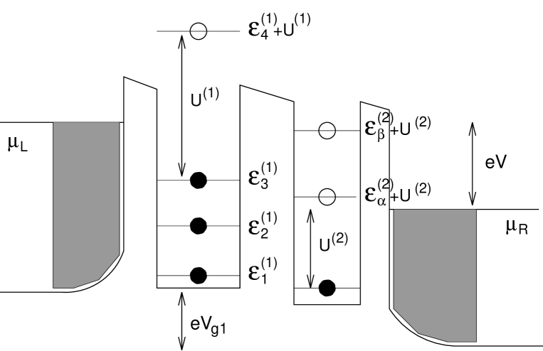
FIG. 1.: Schematic energy potential landscape of the double quantum dots and leads. $\epsilon^{(i)}_{l_{i}}$’s ($i=1,2$) are the energy spectra in dot-1 and dot-2, respectively. The solid and empty dots represent populated and unpopulated states. $U^{(i)}$, a charging energy, produces populated states separated from the empty states. $V_{g1}$ is a gate voltage applied to dot-1. $V$ is a bias voltage.

Fig.1 of PRB, Zang et al

FIG. 2.: Current through the DQD vs. gate voltage $V_{g1}$ using a bias voltage $V=280\mu V$. $|t|=0.2\mu eV$; $\Delta E^{(1)}=150\mu eV$; $\Delta E^{(2)}=230\mu eV$

Fig.2 of PRB, Zang et al

FIG. 3.: Tunneling current peak splitting vs. coupling $|t|$ and varying gate voltage $V_{g}$ for a symmetrical double-dot: $\Gamma_{1}=\Gamma_{2}\equiv\Gamma$ and $\epsilon^{(1)}_{1}=\epsilon^{(2)}_{2}$.

Fig.3 of PRB, Zang et al

REFERENCES

- [1] M. Kemerinck and L.W. Molenkamp, Appl. Phys. Lett. 65, 8 (1994).
- [2] N.C. van der Vaart et al, Phys. Rev. Lett. 74, 4702 (1995).
- [3] F. R. Waugh et al, Phys. Rev. Lett. 75, 705 (1995).
- [4] I.M. Ruzin et al, Phys. Rev. B 45, 13469 (1992).
- [5] G. Klimeck, G. Chen, and S. Datta, Phys. Rev. B 50, 2316 (1994); G. Chen et al, ibid, 50, 8035 (1994).
- [6] C.A. Stafford and S. Das Sarma, Phys. Rev. Lett. 72, 3590 (1994).
- [7] C. Niu, L. Liu, and T. Lin, Phys. Rev. B 51, 5130 (1995).
- [8] K. A. Matveev, L. I. Glazman, and H. U. Baranger, preprint.
- [9] J. M. Golden and B. I. Halperin, preprint.
- [10] Y. Meir and N. S. Wingreen, Phys. Rev. Lett. 68, 2512 (1992).
- [11] J. Zang and J. L. Birman, Phys. Rev. B 47, 10654 (1993); J. Zang, Ph.D. thesis, CUNY (1994).
- [12] S. Hershfield, J. H. Davies, and J. W. Wilkins, Phys. Rev. Lett. 67, 3720 (1991); S. Hershfield, J. H. Davies, and J. W. Wilkins, Phys. Rev. B 46, 7046 (1992).
- [13] Y. Meir, N. S. Wingreen, and P. A. Lee, Phys. Rev. Lett. 66, 3048 (1991).
- [14] A. Groshev, T. Ivanov, and V. Valtchinov, ibid., 66, 1082 (1991).
- [15] J. Faist et al, Science 264, 553 (1994).
- [16] P. Martin and J. Schwinger, Phys. Rev. 115, 1342 (1959); L.P. Kadanoff and G. Baym, Quantum Statistical Mechanics (Benjamin, NY, 1962); P.M. Bakshi and K.T. Mahanthappa, J. Math. Phys. 4, 12 (1963).
- [17] L.V. Keldysh, Sov. Phys. JETP 20, 1018 (1965).
- [18] J. Rammer and H. Smith, Rev. Mod. Phys. 58, 323 (1986); K. C. Chou, Z. B. Su, B. L. Hao, and L. Yu, Phys. Rep. 118, 1 (1985).
- [19] In cases is not diagonal in the space, one need to re-define the basis states, then current equation is still given by Eq.(11).
- [20] L. Wang, J. K. Zhang, and A. R. Bishop, Phys. Rev. Lett. 73, 585 (1994); ibid., 74, 4710 (1995).
- [21] When , the population in the resonance level of dot-1 will be reduced near resonance, while that in dot-2 will increase.
- [22] For a review, see M. A. Kastner, Rev. Mod. Phys. 64, 849 (1992).
- [23] In Fig.2 of Ref.[3], the authors also observed peak splitting for small inter-dot conductance. It is difficult to judge whether or not. From Fig.3 of Ref.[3], the smallest , which gives peak splitting ( according to our calculation). Considering , should be smaller than to observe resonance. A reasonable interpretation is that for the smallest peak splitting in [3] the inter-dot tunneling is .
- [24] R. F. Kazarinov and R.A. Suris, Sov. Phys. Semicond. 5, 707 (1991).
- [25] A. Kastalsky, V.J. Goldman, J. Abeles, Appl. Phys. Lett. 59, 2636 (1991).