The three species monomer-monomer model:
A mean-field analysis and Monte Carlo study

Abstract

We study the phase diagram and critical behavior of a one dimensional three species monomer-monomer catalytic surface reaction model. Static Monte Carlo simulations are used to roughly map out the phase diagram consisting of a reactive steady state bordered by three equivalent unreactive phases where the surface is saturated with one monomer species. The transitions from the reactive phase are all continuous, while the transitions between poisoned phases are first-order. Of particular interest are the bicritical points where the reactive phase simultaneously meets two poisoned phases. A mean-field cluster analysis fails to predict all of the qualitative features of the phase diagram unless correlations up to triplets of adjacent sites are included. Scaling properties of the continuous transitions and the bicritical points are studied using dynamic Monte Carlo simulations. The transition from the reactive to a saturated phase shows directed percolation critical behavior, while the universal behavior at the bicritical point is in the even branching annihilating random walk class. The crossover from bicritical to critical behavior is also studied.

I Introduction

Nonequilibrium models with many degrees of freedom whose dynamics violate detailed balance arise in studies of biological populations, chemical reactions such as heterogeneous catalysis, fluid turbulence, and elsewhere. The macroscopic behavior of these models can be much richer than that of systems in thermal equilibrium, showing organized macroscopic spatial and temporal structures like pulses or waves, and even spatiotemporal chaos. Even the steady state behavior can be far more complicated, involving for example scale invariance at generic parameter values, and critical behavior distinct from any equilibrium models. However, like their equilibrium cousins, systems at continuous transitions between nonequilibrium steady states show universal behavior that is insensitive to microscopic details and depends only on properties such as symmetries and conservation laws.

One place where such nonequilibrium models appear is in the study of chemical reactions occurring on catalytic surfaces, which show a variety of interesting behavior including nonequilibrium phase transitions, temporal oscillations, spiral waves, and chemical chaos[1]. In order to help understand these complicated processes, a number of simple models have recently been proposed that attempt to capture the essential physics[2].

Ziff, Gulari, and Barshad (ZGB) proposed a monomer-dimer reaction model to explain some features of CO oxidation on a noble metal surface [3]. In their model, monomers representing CO molecules and dimers representing O₂ molecules adsorb on a lattice. Immediately upon adsorption, the O₂ dimers dissociate into two O monomers. CO monomers and O monomers occupying nearest neighbor sites then react to form a CO₂ molecule that immediately desorbs, leaving two vacant lattice sites. In the limit of infinitely fast reactions (the adsorption controlled limit), where the only parameter of the model is the relative adsorption rate of CO molecules $y_{CO}$, they found in two dimensions that there are three phases: An O₂, or dimer poisoned state for $y_{CO}<y_{1}$, a CO, or monomer poisoned phase for $y_{CO}>y_{2}$, and a reactive phase for $y_{1}<y_{CO}<y_{2}$. At $y_{1}$ the fraction of each species changes continuously, indicating that the dimer poisoning transition is continuous. At $y_{2}$ the monomer poisoning transition is first order, with the densities of the different species changing discontinuously. In one dimension, the ZGB monomer-dimer reaction model has no reactive phase, only monomer-poisoned and dimer-poisoned phases separated by a first-order transition[4].

An even simpler catalytic reaction model can be constructed by replacing the dimer species in the ZGB model with a second monomer species. This monomer-monomer model has a long history[5], and in fact certain analytic results for this model have been obtained in the reaction-controlled limit of the model[6]. In this model two different monomer species, call them A and B, adsorb on a lattice where nearest neighbor AB pairs react and an AB molecule desorbs. However, the phase diagram for this model does not contain a reactive steady state in any number of dimensions, neither in the adsorption controlled nor in the reaction controlled limit. The phase diagram consists only of A and B poisoned states, and a first-order transition between them.

The dimer poisoning transition in the ZGB model is one of the most common types of continuous phase transitions in nonequilibrium models. It is a transition to a single absorbing, noiseless, steady state, the term absorbing indicating the state cannot be left once it is reached. Other examples include directed percolation (DP)[7, 8], the contact process[9], auto-catalytic reaction models[10], and branching annihilating random walks with odd numbers of offspring[11, 12]. Both renormalization group calculations[7, 13] and Monte Carlo simulations[8, 9, 10, 11, 12, 14] show that these models form a single universality class for a purely nonequilibrium model with no internal symmetry in the order parameter.

Recently, a number of models with continuous adsorbing transitions in a universality class distinct from directed percolation have been studied. These models include probabilistic cellular automata models studied by Grassberger et al.[15], certain kinetic Ising models [16], the interacting monomer-dimer model[17, 18], and branching annihilating random walks with an even number of offspring (BAWe)[11, 19]. All of these models except for the BAWe have two equivalent absorbing states indicating the importance of symmetry of the adsorbing state to the universality class. However, the universal behavior of this new class is apparently controlled by a dynamical conservation law. If the important dynamical variables in this class are defects represented by the walkers in the BAWe model and the walls between different saturated domains in the other models, the models have a “defect parity” conservation law[15] where the number of defects is conserved modulo 2. Recent field theoretic work confirms this viewpoint[20].

In a recent Letter[21], we introduced a monomer-monomer reaction model with three different monomer species. This model could represent either a system with three different chemical species or an auto-catalytic reaction system in which one chemical species can adsorb on three different types of surface sites. Using static and dynamic Monte Carlo simulations, we determined the phase diagram and studied the phase transitions in the one dimensional version of the model, and showed that it has continuous adsorbing transitions to both one and two equivalent noiseless states. It is therefore is a good model to study the role of symmetry in adsorbing phase transitions.

In this paper we expand those results, providing more details of our simulation methods and of the results, again restricting our consideration the the one-dimensional version of the model. We also include a mean-field cluster analysis of the model including up to triplets of adjacent sites. The paper is organized as follows. In the next section we define the model and show the phase diagram of the model, as determined by simulations. The following section presents the mean-field analysis. Section IV contains the details and results a detailed Monte Carlo study of the dynamic scaling behavior at the various phase transitions, and of the crossover behavior between the different types of scaling behavior. In the last section we summarize our results.

II The model

Our three species monomer-monomer model is defined by two fundamental dynamic processes: (a) monomer adsorption at sites of a substrate, and (b) the annihilation reaction of two dissimilar monomers adsorbed on nearest-neighbor sites of the substrate. Here we consider the model only in the adsorption controlled limit where process (b) occurs instantaneously. Calling the monomer species $A$, $B$ and $C$, the parameters in the model are then the relative adsorption rates of the different monomer species $p_{A}$, $p_{B}$, and $p_{C}$, such that $p_{A}+p_{B}+p_{C}=1$. Using static Monte Carlo simulations to get the rough picture, and refining it with dynamical Monte Carlo studies described below, we find the ternary phase diagram for the model is shown in Fig. 1. In this figure, the horizontal axis corresponds to the relative adsorption rate of $A$ and $B$ monomers $p_{AB}=p_{A}/(p_{A}+p_{B})$. The absorbing phases, where one monomer species saturates the chain, occupy the corners of the phase diagram. In the center of the phase diagram is a a reactive steady state. There are continuous phase transitions from the reactive phase to the saturated phases, but the monomer densities undergo discontinuous, first-order, transitions from one saturated state to another. The points where the reactive phase and two saturated phases meet are bicritical points[22] where two lines of continuous transitions meet a line of first-order transitions.

III Mean-field theory

To analyze the kinetics of the three species monomer-monomer model, it is useful to perform a mean-field analysis. While such analysis neglects long-range correlations and thus cannot be expected to properly predict critical properties, it should properly predict the qualitative structure of the phase diagram, including the existence of continuous transitions and multi-critical points. The mean-field analysis also provides a starting point for studying the importance of such fluctuations, which, of course, become particularly important near continuous phase transitions. The mean-field approach we use[23] studies the time evolution of clusters of sites, the approximation coming in truncating the probabilities of observing clusters of larger size into probabilities for smaller size clusters. The simplest form is the site approximation where probabilities of observing certain nearest neighbor pairs is replaced by the produce of the average site densities. Better approximations can be obtained systematically by replacing the actual configuration of larger clusters, i.e. pairs, then triplets, and so on, with the average density of those clusters. The analysis presented below includes clusters consisting of up to triplets of adjacent sites.

A Site approximation

At a particular time, a lattice with $N$ sites will have $N_{V}$ vacancies, the remaining sites being filled with $N_{A}$, $N_{B}$, and $N_{C}$ numbers of $A$, $B$, and $C$ monomers respectively. The density of $A$ monomers is $x_{A}\equiv(N_{A}/N)$, with corresponding definitions for $B$, $C$ and vacant ($V$) sites. We have the obvious constraint

$$x_{V}+x_{A}+x_{B}+x_{C}\equiv 1.$$ (1)

In the site approximation all correlations are neglected, so that $x_{V}^{2}$ is the probability that a given pair of lattice sites are occupied by two vacancies. The rate equations for the $A$ monomer density is

$${dx_{A}\over dt}=p_{A}x_{V}(1-x_{B}-x_{C})^{2}-(p_{B}+p_{C})x_{V}\left[1-(1-x_{A})^{2}\right]$$ (2)

with similar equations for $x_{B}$ and $x_{C}$. The first term on the right hand side of Eq. (2) is the rate of $A$ monomer adsorption multiplied by the probability that an adsorbing $A$ monomer will find a vacant site that has no $B$ or $C$ monomers adsorbed on adjacent sites. The second term is the rate at which $B$ or $C$ monomers find a vacant site with at least one adjacent adsorbed $A$ monomer to react with.

Equations (2) have steady state solutions corresponding to each of the three poisoned states, as well as one corresponding to the reactive steady state. To find the site approximation phase diagram, we analyzed the stability of those solutions as a function of the rates $\{p_{\alpha}\}$ by examining the eigenvalues of the Jacobian matrix for linearized rate equations.

For example, the Jacobian matrix for the $A$ poisoned state has two zero eigenvalues and one eigenvalue of $p_{B}+p_{C}-p_{A}=(1-2p_{A})$. This third eigenvalue shows that the $A$ poisoned state is stable only for $p_{A}>1/2$. Corresponding results hold for the other poisoned states, leading to the site approximation phase diagram shown in Fig. 2.

As the phase boundaries are approached from the reactive phase, the monomer densities vanish continuously, indicating a continuous transition to an absorbing state. The points on the edge of the phase diagram where two different poisoned phases meet the reactive phase are bicritical points.

B Pair approximation

We improve the site approximation by properly accounting for the correlation of nearest neighbor pairs and approximating the correlations of triples and larger clusters. We define $N_{ij}$ as the number of bonds connecting nearest neighbor sites occupied by $i$ and $j$ monomers ($A$, $B$, $C$, or $V$), where the monomer $i$ occupies the site to the left of monomer $j$, and we have $N_{ij}=N_{ji}$. Since we are studying one dimension, the number of bonds equals the number of sites $N$, so the bond densities are defined by

$$x_{ij}\equiv{N_{ij}+N_{ji}\over N},\qquad\qquad i\neq j$$

and

$$x_{ii}\equiv{N_{ii}\over N}$$

There are seven different allowed types of bonds: V-V, A-A, B-B, C-C, A-V, B-V, and C-V. Other types of bonds, A-B, A-C, and B-C, are forbidden in the adsorption controlled limit we are considering. The densities satisfy the constraint

$$x_{VV}+x_{AA}+x_{BB}+x_{CC}+x_{AV}+x_{BV}+x_{CV}=1,$$ (3)

so only six of the $x_{ij}$ are independent. The $A$ monomer density is given by $x_{A}=x_{AA}+{1\over 2}x_{AV}$, with similar expressions for the $B$ and $C$ densities.

To determine the equations of motion of the pair densities it is useful to distinguish between the different types of events that change the configuration. For example, if an $A$ monomer attempts to occupy a site, it can (1) stick, (2) react with a $B$ or (3) react with a $C$, which we indicate respectively with the shorthand : (1) $A\downarrow$, (2) $A\downarrow\;AB\uparrow$, and (3) $A\downarrow\;AC\uparrow$. The rate equations can be written as

$${dx_{ij}\over dt}=\sum_{\alpha}\Delta x_{ij}^{(\alpha)}$$

where $\alpha$ refers to the event type, and $\Delta x_{ij}^{(\alpha)}$ is the change in $ij$ bond density arising from an event of type $\alpha$.

To find the different bond density changes note that the probability $P(i|j)$ for a site to be occupied by a monomer (or vacancy) of type $i$, given that one of its nearest neighbors is of type $j$, is

$$P(i|j)={N_{ij}\over N_{i}}={x_{ij}\over 2x_{j}}$$

for $i\neq j$, and

$$P(i|i)={x_{ii}\over x_{i}}$$

The various $\Delta x_{ij}^{(\alpha)}$ are given in Table 1, where

$$z_{iV}=P(i|V)+P(V|V)={x_{VV}+{1\over 2}x_{iV}\over x_{V}}$$

is the probability that the site to the left of a vacant site is occupied by either an $i$ type monomer or a $V$. The density changes due to the other event types are found by permutation.

Thus, the rate equations are

$${dx_{AA}\over dt} = p_{A}\;x_{AV}\;z_{AV}-{x_{AA}x_{AV}\over 2x_{A}}\left[p_{B}(1+z_{BV})+p_{C}(1+z_{CV})\right]$$ (4)

$${dx_{AV}\over dt} = p_{A}\;z_{AV}(2x_{VV}-x_{AV})-{x_{AV}^{2}\over 2x_{A}}\left[p_{B}(1+z_{BV})+p_{C}(1+z_{CV})\right]$$ (5)

The other equations can be found by permutation, except for $x_{VV}$ which can be found using Eq. (3).

Multiple steady state solutions to the set of six coupled bond density rate Eqs. (5) correspond to the reactive state (which can be found numerically), as well the three poisoned states. In principle, to find the phase diagram a stability analysis of those steady state solutions could be performed. However, we instead simply solved the six equations numerically as a function of the parameters $p_{AB}$ and $p_{C}$, and looked for the transitions to the poisoned states. The results are shown in Fig. 3. The densities of the different monomer species still change continuously as the phase boundaries are approached, indicating that the transitions are continuous. While the phase boundaries are now curved as they are in the actual phase diagram, the bicritical points are still on the edge of the phase diagram unlike the actual phase diagram.

C Triplet approximation

The mean-field theory can be refined even further by considering larger clusters. However, this systematic process rapidly increases in difficulty. But since even the pair approximation failed to predict that the bicritical points occur on the interior of the phase diagram, we pushed the cluster expansion one step further and analyzed the model in the triplet approximation. In this approximation, clusters of three adjacent sites are considered, thereby including the effects of correlations up to that level. The details of the calculation are presented in the Appendix, but here we summarize the results. In one dimension, there are 19 different allowed triplets. However, 4 different constraints reduce the number of independent triplets to 15. Numerically solving the rate equations for the densities of those 15 different triplets simultaneously, we find solutions corresponding to the reactive steady state, as well as the poisoned states. The phase diagram, calculated as for pair approximation, is shown in Fig. 4. Finally at this level of approximation all of the qualitative features of the actual phase diagram are predicted. In particular, the bicritical points appear on the interior of the phase diagram and there are first order lines between the poisoned phases. However, note that the size of the poisoned phases is still underestimated by the mean-field cluster analysis, even in the triplet approximation. For example, the bicritical point on the $p_{AB}=0.5$ line occurs at about $p_{C}=0.02$ in the triplet approximation, whereas in actuality it occurs at about $p_{C}=0.12$. This indicates that fluctuations, which are still not fully accounted for in mean-field theory, stabilize the poisoned phases.

IV Simulations

To further investigate the three species monomer-monomer model we also used time-dependent Monte Carlo simulations. Particularly useful for studying critical properties, the method is a form of “epidemic” analysis[12, 19, 24] in which the average time evolution of a particular configuration that is very close to an adsorbing state (defect dynamics), or very close to a minimal width interface between two different adsorbing states (interface dynamics), is measured by simulating a large number of independent realizations. Using this technique we determined the universality classes of the critical and bicritical points, and studied the critical dynamics of interfaces between the two symmetric saturated states at the bicritical points, and the crossover from bicritical to critical behavior, including measuring the crossover exponent $\phi$, as well as the subcritical behavior at the first-order lines.

Because monomers can adsorb only at vacant sites, and the total number of vacancies on the lattice is usually very small, instead of randomly picking a site to attempt to adsorb on, it is much more efficient to use a variable time algorithm in which the adsorption site is randomly picked from a list of vacant sites. The species of monomer chosen for adsorption is then randomly picked according to the relative adsorption rates $\{p_{\alpha}\}$, and the time length of a step is $1/n_{V}(t)$ where $n_{V}(t)$ is the total number of vacancies at that time. Thus, on average there is one attempted adsorption per lattice site per unit time. We always start with a lattice big enough that the active region will never reach the boundaries; it is effectively an infinite lattice.

During the simulations we measured the survival probability $P(t)$, defined as the probability that the system had not poisoned by time $t$, the average number of vacancies per run $\langle{n}_{V}(t)\rangle$, and the average mean-square size of the active region per surviving run $\langle{R^{2}}(t)\rangle$. At a continuous phase transition as $t\rightarrow\infty$ these dynamical quantities obey power law behavior

$$P(t)\sim t^{-\delta},\qquad\langle{n}_{V}(t)\rangle\sim t^{\eta},\qquad\langle{R^{2}}(t)\rangle\sim t^{z}.$$ (6)

Plots of the logarithms of these quantities versus the logarithm of the time, such those shown in Fig. 5 yield a straight line at the phase transition, and show curvature away from the transition.

Precise estimates of the location of the critical point and of the exponents can be made by examining the local slopes of the curves on a log-log plot. The effective exponent $\delta(t)$ is defined as

$$-\delta(t)=\{\ln\left[P(t)/P(t/b)\right]/\ln b\}\,,$$ (7)

with similar expressions for $\eta(t)$ and $z(t)$. At the critical point, a graph of the local slope versus $t^{-1}$ should extrapolate to the critical exponent, with a correction that is expected[25] to be linear in $t^{-1}$. Away from the critical point, the local slope curve should show strong curvature away from the critical point value as $t^{-1}\to 0$.

A Critical dynamics

Figure 5 shows the data for the three dynamic quantities near the phase transition to the $C$ saturated phase at $p_{AB}=0.5$ plotted against time on a log-log scale. This data was calculated from $10^{5}$ independent runs of up to $10^{4}$ time steps at each parameter value. As expected, right at the critical point the line is straight, indicating power law scaling, and away from the critical point the lines show curvature.

The exponents and the location of the critical point are easily and precisely determined by taking the local slopes of this data, which are shown in Fig. 6. We find a critical $C$ monomer adsorption rate of $\tilde{p}_{C}=0.39575(10)$, and that the critical exponents are $\delta=0.16(1)$, $\eta=0.31(1)$, and $z=1.255(15)$. These values are consistent with our expectation that this transition should be in the DP universality class, for which the exponents are $\delta=0.1596(4)$, $\eta=0.3137(10)$, and $z=1.2660(14)$[26]. We found similar exponents for the adsorbing transition at a number of other points along the lines separating the reactive phase and the saturated states (see the discussion of the crossover from bicritical to critical behavior below), indicating the transition between the reactive phase and any single saturated phase is always in the DP universality class.

B Bicritical defect dynamics

The same kind of analysis at the bicritical point at $p_{AB}=0.5$, using an initial condition of a vacancy in an A-saturated phase, yields a bicritical point at $p_{C}=p_{C}^{*}=0.122(1)$. The exponents at the bicritical point are very different, which we expect given the presence of two-symmetry equivalent saturated phases. From $5\times 10^{5}$ runs of up to $10^{5}$ time steps we found the local slope data shown in Fig. 7, yielding values of $\delta=0.29(1)$, $\eta=0.00(1)$, and $z=1.150(15)$. These values indicate that the bicritical behavior falls in the BAWe universality class, for which $\delta=0.285(2)$, $\eta=0.000(1)$, and $z=1.141(2)$[19].

For $p_{C}<p^{*}_{C}$ along the A-B coexistence line, a similar analysis shows a crossover from the bicritical behavior to sub-critical behavior corresponding to the well known problem of the $T=0$ one-dimensional kinetic Ising model for which dynamic exponents $\delta=0.5$, $\eta=-0.5$, and $z=1$ are known exactly[27]. The two species version of our model, which occurs for $p_{C}=0$ on the edge of the phase diagram, can be mapped onto this kinetic Ising Model. However, as can be seen in Fig. 8, for $0<p_{C}<p^{*}_{C}$ at short times the dynamic critical behavior tends to act more like the bicritical behavior before changing to kinetic Ising model behavior at long times. The time which this crossover occurs increases as $p_{C}$ approaches $p^{*}_{C}$, but for all $p_{C}<p^{*}_{C}$ the long time dynamical critical behavior corresponds to the kinetic Ising model.

C Bicritical interface dynamics

To further analyze the importance of competition in the growth of two equivalent saturated phases at the bicritical point we also studied the dynamics of an interface between those two phases. Starting with a single vacancy between the two domains, we used two different methods to analyze the behavior of the interface. Since there must always be at least one vacancy between two different saturated phases, in the first method we ignore the survival probability $P(t)$ and take $\delta\equiv 0$. We then measure the number of vacancies in the interface $\langle n(t)\rangle\propto t^{\eta}$ and average size of the interface $\langle R^{2}(t)\rangle\propto t^{z}$. From $5\times 10^{4}$ independent runs at the bicritical point, each lasting $10^{5}$ time steps, we found the other exponents to be $\eta=0.285(10)$ and $z=1.14(2)$. This type of interface dynamics has been used to study the properties of critical interfaces in other models in the BAWe class, where similar results for $\eta$ and $z$ were obtained[18, 19].

In the second type of interface dynamics simulations, which has not been studied before, the simulation is stopped if the interface between the domains has “collapsed” back to one vacant site. We introduce a probability of avoiding a collapse $P(t)\propto t^{-\delta^{\prime}}$ and corresponding vacancy concentrations $\langle n(t)\rangle\propto t^{\eta^{\prime}}$ and $\langle R^{2}(t)\rangle\propto t^{z^{\prime}}$. Figure 9 shows results from $10^{7}$ independent runs each lasting up to $10^{5}$ time steps. We find values of $\delta^{\prime}=0.73(2)$, $\eta^{\prime}=-0.43(2)$ and $z^{\prime}=1.15(2)$.

Note the value of the dynamic exponent $z$ or $z^{\prime}$, which measures the size of the active region during surviving runs, is the same in both types of interface dynamics simulations as that measured for the defect dynamics. Furthermore, although the exponents $\delta$ and $\eta$ are different in the three cases, their sum $\delta+\eta$ (or $\delta^{\prime}+\eta^{\prime}$), which governs the time evolution of the number of vacancies in just the surviving runs, are the same within statistical error. This indicates a universal nature of the critical spreading of the active region for models with two symmetric adsorbing states which is independent of whether defect or interface dynamics is being considered. A similar result holds for some one-dimensional systems with infinitely many adsorbing states[28].

Assuming this conjecture is true, it should be noted that simulations using the first type of interface dynamics, where $\delta\equiv 0$, yield no information beyond that obtainable from simulations employing defect dynamics. However, simulations using the second type of interface dynamics measure an independent dynamic exponent $\delta^{\prime}$ which we expect to be a universal number. Recent measurements on similar models support this conjecture [29].

D Crossover from bicritical to critical behavior

Finally, we measured the crossover exponent from bicritical to critical behavior. Near the bicritical point where the A and B poisoned phases meet, the boundary of the reactive region is expected to behave as $(p_{AB}-0.5)\propto(p_{C}-p^{*}_{C})^{\phi}$, where $\phi$ is the crossover exponent[22]. We used the dynamical simulation method to accurately determine the location of the DP phase boundary between the reactive phase and the $A$ saturated phase near the bicritical point. From the log-log plot of $p_{AB}-0.5$ versus $p_{C}-p^{*}_{C}$ shown in Fig. 10, we find $\phi=2.1\pm 0.1$. Our determination of $\phi$ is not as accurate as the other exponents due to complications arising from crossover effects. Similar to the crossover from bicritical to sub-critical behavior described above, near the bicritical point at short times the dynamical behavior is controlled by the bicritical point before changing to the directed percolation critical behavior at long times. The time with which the crossover occurs increases as the bicritical point is approached, making studies very close to the bicritical point too time-consuming.

V Summary

We have studied a simple three species monomer-monomer reaction model to investigate the role of symmetry in adsorbing phase transitions. We have shown that, unlike the two species monomer-monomer model or the monomer-dimer ZGB model, this model has a reactive steady state in one dimension. There are also poisoned states for which the lattice is covered by one of the monomer species. The continuous phase transitions between the reactive phase and the poisoned states meet at bicritical points. Along the first-order coexistance line between two absorbing phases the model reduces to the two species monomer-monomer model.

We also constructed a mean-field theory of the model. An unusual feature of the mean-field analysis is that the bicritical points lie on the edge of the phase diagram if the correlations of triplets of adjacent sites are not exactly treated. Only when correlations up to triplets of adjacent sites are included does the bicritical point appear inside the phase diagram, indicating the importance of reproducing the correlations induced by large domains of a single saturated phase.

The dynamic critical behavior at the transition between the reactive phase and a poisoned phase is in the DP universality class. At the bicritical points, where there are two equivalent poisoned states, the dynamic critical behavior is in the BAWe class. Thus, the universality class of the transition changes from DP to BAWe when the symmetry of the adsorbing state is increased from one to two equivalent noiseless states. Furthermore, we have shown that having a two-fold symmetry in the adsorbing states introduces additional features in the dynamics over a model with a unique adsorbing state. In particular, the critical dynamics of the interfaces between two different adsorbing states shows a sensitivity to how the dynamics is defined, and the survival probability of fluctuations in the size of the interface from its smallest value is described by a new universal exponent $\delta^{\prime}$. However, the critical spreading of the reactive region, be it a defect in a single phase or a domain wall between phases, appears to be insensitive to the choice of initial conditions. This appears to result from the fact that large reactive regions are insensitive to whether the reactive regions are bounded by the same or different saturated phases. We do not expect this result to be true in higher dimensions where the entropy of domain walls can play a role and nonuniversal critical spreading has been observed in other models[30].

This work was supported by the National Science Foundation under Grant No. DMR–9408634.

Rate equations in the triplet approximation

The triplet approximation replaces the actual lattice configuration with the average configuration of each cluster consisting of a three adjacent sites. Define the average number of the different number of triplets as

$$x_{ijk}\equiv{N_{ijk}\over N}$$

where $N$ is the total number of triplets, which in one dimension is equal to the the number of sites, and $N_{ijk}$ is the number of triplets consisting of $i$, $j$, and $k$ type monomers ($A$, $B$, or $C$) or vacancies ($V$). The densities of asymmetric triplets, i.e. $ijk$ type triplets with $i\neq k$, are by symmetry assumed to be equal, and are added together.

In the adsorption controlled limit, triplets with adjacent dissimilar monomers, e.g. A-B-B, A-C-V, …, are forbidden, leaving 19 allowed types of triplets. However, the triplet densities must satisfy 4 separate constraints, which reduce the number of independent triplet densities to 15. The first of these constraints, similar to the constraints on the site and bond densities given by Eq. (1) and Eq. (3) respectively, merely conserves the total triplet density

$$\sum_{ijk}x_{ijk}=1.$$

The other three constraints have no analogues in the site or pair approximations. Because each particular lattice site contributes to three different triplets, and the middle and end positions of the triplets are not symmetric, the total density of $A$ type monomers occurring in say the left position of the triplets must be equal to the the total density of $A$ type monomers occurring in the middle position of the triplets

$$x_{AVV}+2x_{AVA}+x_{AVB}+x_{AVC}=x_{AAV}+2x_{VAV},$$

and similarly for $B$ and $C$ type monomers.

The equations of motion of the triplet densities can be written as

$${dx_{ijk}\over dt}=\sum_{\alpha}\Delta x_{ijk}^{(\alpha)}$$

where $\alpha$ refers to the event type, and $\Delta x_{ijk}^{(\alpha)}$ are the triplet density changes with an event of type $\alpha$. The different types of events were enumerated above in the discussion of the pair approximation. The triplet density changes due to $A\downarrow$ and $A\downarrow\;AB\uparrow$ events are listed in Tables II and III, respectively, where

$$y_{AB}\equiv x_{BVV}+x_{BVB}+x_{AVB}+{1\over 2}x_{BVC}$$

and $P_{ijk/Xjk}$ is the conditional probability for an $i$ type monomer or vacancy to occur next to a $jk$ pair. For example,

$$P_{VVV/XVV}={x_{VVV}\over x_{VVV}+{1\over 2}x_{AVV}+{1\over 2}x_{BVV}+{1\over 2}x_{CVV}}$$

and

$$P_{VAV/XAV}={x_{VAV}\over x_{VAV}+{1\over 2}x_{AAV}}.$$

Then taking $x_{VVV}$, $x_{AVV}$, $x_{BVV}$, and $x_{CVV}$ to be the dependent triplet densities, the equations of motion of the independent triplet densities are

$${dx_{AAA}\over dt} = p_{A}\left[x_{AVA}+\left(2x_{AVA}+x_{AVV}\right)\;P_{AAV/XAV}\right]$$ (9)

$$-\left(p_{B}\;y_{BA}\;+p_{C}\;y_{CA}\right)\;P_{AAV/XAV}\;P_{AAA/XAA}$$

$${dx_{AAV}\over dt} = p_{A}\left[x_{AVV}+\left(2x_{AVA}+x_{AVV}\right)\;\left(P_{VAV/XAV}-P_{AAV/XAV}\right)\right]$$ (11)

$$+\left(p_{B}\;y_{BA}\;+p_{C}\;y_{CA}\right)\;P_{AAV/XAV}\;\left(-1+P_{AAA/XAA}-P_{AAV/XAA}\right)$$

$${dx_{VAV}\over dt} = p_{A}\left[x_{VVV}-\left(2x_{AVA}+x_{AVV}\right)\;P_{VAV/XAV}\right]$$ (13)

$$-\left(p_{B}\;y_{BA}+p_{C}\;y_{CA}\right)\;\left(P_{VAV/XAV}-P_{AAV/XAV}\;P_{AAV/XAA}\right)$$

$${dx_{AVA}\over dt} = p_{A}\left[-x_{AVA}+\left(2x_{VVV}+x_{AVV}\right)\;P_{AVV/XVV}\right]$$ (16)

$$-\left(p_{B}+p_{C}\right)\;x_{AVA}$$

$$-\left(p_{B}\;y_{BA}+p_{C}\;y_{CA}\right)\;P_{VAV/XAV}\;P_{AVA/AVX}$$

$${dx_{AVB}\over dt} = p_{A}\;\left(2x_{VVV}+x_{AVV}\right)\;P_{BVV/XVV}$$ (22)

$$+p_{B}\;\left(2x_{VVV}+x_{BVV}\right)\;P_{AVV/XVV}$$

$$-p_{A}\;x_{AVB}-p_{A}\;y_{AB}\;P_{VBV/XBV}\;P_{AVB/BVX}$$

$$-p_{B}\;x_{AVB}-p_{B}\;y_{BA}\;P_{VAV/XAV}\;P_{AVB/AVX}$$

$$-p_{C}\;x_{AVB}$$

$$-p_{C}\;y_{CA}\;P_{VAV/XAV}\;P_{AVB/AVX}-p_{C}\;y_{CB}\;P_{VBV/XBV}\;P_{AVB/BVX}$$

and similarly for the remaining densities.

event type	$A\downarrow$	$A\downarrow\;AB\uparrow$
$\Delta x_{VV}$	$-2\;p_{A}\;z_{AV}\;x_{VV}$	${1\over 2}p_{A}\;x_{BV}\;(1+z_{AV})\left[1+{x_{BV}\over 2x_{B}}\right]$
$\Delta x_{AA}$	$p_{A}\;z_{AV}\;x_{AV}$	$0$
$\Delta x_{BB}$	$0$	$-{1\over 2}p_{A}\;x_{BV}(1+z_{AV}){x_{BB}\over x_{B}}$
$\Delta x_{CC}$	$0$	$0$
$\Delta x_{AV}$	$p_{A}\;z_{AV}(2x_{VV}-x_{AV})$	$0$
$\Delta x_{BV}$	$0$	$-{1\over 2}p_{A}\;x_{BV}(1+z_{AV}){x_{BV}\over x_{B}}$
$\Delta x_{CV}$	$0$	$0$

TABLE I.: Bond density changes for different events in the pair approximation.

event type	$A\downarrow$
$\Delta x_{VVV}$	$-p_{A}\left[x_{VVV}+(2x_{VVV}+x_{AVV})P_{VVV/XVV}\right]$
$\Delta x_{AAA}$	$p_{A}\left[x_{AVA}+(2x_{AVA}+x_{AVV})P_{AAV/XAV}\right]$
$\Delta x_{AAV}$	$p_{A}\left[x_{AVV}+(2x_{AVA}+x_{AVV})(P_{VAV/XAV}-P_{AAV/XAV})\right]$
$\Delta x_{VAV}$	$p_{A}\left[x_{VVV}-(2x_{AVA}+x_{AVV})P_{VAV/XAV}\right]$
$\Delta x_{AVA}$	$p_{A}\left[-x_{AVA}+(2x_{VVV}+x_{AVV})P_{AVV/XVV}\right]$
$\Delta x_{AVV}$	$p_{A}\;\left[-x_{AVV}+(2x_{VVV}+x_{AVV})(P_{VVV/XVV}-P_{AVV/XVV})\right]$
$\Delta x_{BVV}$	$-p_{A}(2x_{VVV}+x_{AVV})P_{BVV/XVV}$
$\Delta x_{CVV}$	$-p_{A}(2x_{VVV}+x_{AVV})P_{CVV/XVV}$
$\Delta x_{AVB}$	$p_{A}(2x_{VVV}+x_{AVV})P_{BVV/XVV}$
$\Delta x_{AVC}$	$p_{A}(2x_{VVV}+x_{AVV})P_{CVV/XVV}$

TABLE II.: Triplet density changes due to an $A$ monomer adsorbing, and remaining on the lattice, in the triplet approximation.

event type	$A\downarrow\;AB\uparrow$
$\Delta x_{VVV}$	$p_{A}\;x_{BVV}+p_{A}\;y_{AB}\;P_{VBV/XBV}(1+P_{BVV/BVX})$
$\Delta x_{BBB}$	$-p_{A}\;y_{AB}\;P_{BBV/XBV}\;P_{BBB/XBB}$
$\Delta x_{BBV}$	$p_{A}\;y_{AB}\;P_{BBV/XBV}\;\left(-1+P_{BBB/XBB}-P_{BBV/XBB}\right)$
$\Delta x_{VBV}$	$-p_{A}\;y_{AB}\;\left(P_{VBV/XBV}-P_{BBV/XBV}\;P_{BBV/XBB}\right)$
$\Delta x_{BVB}$	$-p_{A}\;x_{BVB}-p_{A}\;y_{AB}\;P_{VBV/XBV}\;P_{BVB/BVX}$
$\Delta x_{AVV}$	$p_{A}\;x_{AVB}+p_{A}\;y_{AB}\;P_{VBV/XBV}\;P_{AVB/BVX}$
$\Delta x_{BVV}$	$p_{A}\left[x_{BVB}-x_{BVV}\right]+p_{A}\;y_{AB}\;P_{BBV/XBV}$
	$+p_{A}\;y_{AB}\;P_{VBV/XBV}\;\left(P_{BVB/BVX}-P_{BVV/BVX}\right)$
$\Delta x_{CVV}$	$p_{A}\;{1\over 2}x_{BVC}+p_{A}\;y_{AB}\;P_{VBV/XBV}\;P_{BVC/BVX}$
$\Delta x_{AVB}$	$-p_{A}\;x_{AVB}-p_{A}\;y_{AB}\;P_{VBV/XBV}\;P_{AVB/BVX}$
$\Delta x_{BVC}$	$-p_{A}\;{1\over 2}x_{BVC}-p_{A}\;y_{AB}\;P_{VBV/XBV}\;P_{BVC/BVX}$

TABLE III.: Nonvanishing triplet density changes due to an $A$ monomer adsorbing, and reacting with a $B$ monomer to form a $AB$ molecule, in the triplet approximation.

FIG. 1.: Phase diagram showing three saturated phases (indicated by the letters), and a reactive phase (the unlabeled center region). Solid lines indicate continuous transitions. Dashed lines indicate first-order transitions. Bicritical points (filled circles) occur where two critical lines meet a first-order line.

FIG. 2.: Phase diagram in the site approximation. Transitions between the reactive phase (unlabeled) and the three saturated phases (indicated by the letters) are continuous. Note that unlike the actual phase diagram shown in Fig. 1 the continuous transition lines are straight and the bicritical points where two continuous transition lines meet are on the edge of the phase diagram.

FIG. 3.: Phase diagram in the pair approximation. Transitions between the reactive phase (unlabeled) and the three saturated phases (indicated by the letters) are continuous. Note that unlike the actual phase diagram shown in Fig. 1 the bicritical points are still on the edge of the phase diagram.

FIG. 4.: Phase diagram in the triple approximation. Transitions between the reactive phase and the three saturated phases are continuous, while transitions between saturated phases are first-order. Inset shows a closeup of the phase diagram near the bicritical point at the end of the first-order line separating the A and B saturated phases. All of the qualitative features of the actual phase diagram are reproduced in this approximation.

FIG. 5.: Log-log plot showing the average number of vacancies, $n_{V}$ as a function of time near the transition from the reactive phase to the C saturated phase at $p_{AB}=0.5$. From top to bottom, the 3 curves correspond to $p_{C}=0.395$, 0.39575, and 0.3965. The middle curve corresponds to the critical point. Note that the critical line is straight while the other lines have curvature.

FIG. 6.: Effective exponents using Eq. (7) with $b=5$ for the defect dynamics near the critical point at $p_{AB}=0.5$ on the line where the C poisoned phase meets the reactive phase. From top to bottom, the 3 curves in each panel correspond to $p_{C}=0.3955$, 0.39575, and 0.3960, with the middle curve corresponding to the critical point.

FIG. 7.: Effective exponents using Eq. (7) with $b=5$ for the defect dynamics near the bicritical point where the A and B poisoned phases meet the reactive phase as defined in Eq. (7) with $b=5$. From bottom to top, the 3 curves in each panel correspond to $p_{C}=0.121$, 0.122, and 0.123, with the middle line corresponding to the bicritical point.

FIG. 8.: Average number of vacancies for $p_{AB}=0.5$, and $p_{C}\leq p^{*}_{C}$ showing crossover from bicritical behavior to sub-critical behavior. From bottom to top, the curves correspond to $p_{C}=0.0$, 0.04, 0.08, 0.10, 0.11, and 0.122. The top curve ($p_{C}=0.122$) corresponds to the bicritical point. All other curves tend toward a slope of $-0.5$ at large t.

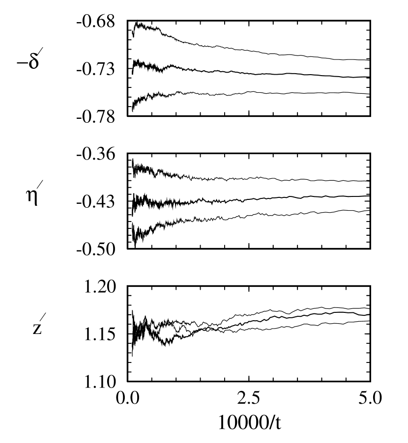
FIG. 9.: Effective exponents, as in Fig. 7, for the second type of interface dynamics near the bicritical point where the A and B poisoned phases meet the reactive phase.

FIG. 10.: Location of the critical line as a function of distance from the bicritical point. The data falls on a line with a slope corresponding to the crossover exponent $\phi=2.1\pm 0.1$.

REFERENCES

- [1] P. Grey and S. K. Scott, Chemical Oscillations and Instabilities (Clarendon, Oxford, 1990); G. Ertl, Adv. Catal. 37, 231 (1990); R. Imbihl and G. Ertl, Chem. Rev. 95, 697 (1995).
- [2] J. Marro and R. Dickman, Nonequilibrium phase transitions in lattice models (Cambridge Univ. Press, 1996).
- [3] R. M. Ziff, E. Gulari, and Y. Barshad, Phys. Rev. Lett. 56, 2553 (1986).
- [4] P. Meakin and D. Scalapino, J. Chem. Phys. 87, 731 (1987).
- [5] E. Wicke, P. Kumman, W. Keil, and J. Scheifler, Ber. Bunsenges. Phys. Chem. 4, 315 (1980); R. M. Ziff and K. A. Fitchthorn, Phys. Rev. B 34, 2038 (1986); K. A. Fitchthorn, E. Gulari, and R. M. Ziff, in: Catalysis 1987, ed. J. W. Ward, (Elsevier, 1987); D. ben-Avraham, D. B. Considine, P. Meakin, S. Redner, and H. Takayasu, J. Phys. A 23, 4297 (1990); D. B. Considine, H. Takayasu, and S. Redner, J. Phys. A 23, L1181 (1990); J. W. Evans and M. S. Miesch, Phys. Rev. Lett. 66, 833 (1991); E. Clément, P. Leroux-Hugon, and L. M. Sander, Phys. Rev. Lett. 67, 1661 (1991); J. W. Evans and T. R. Ray, Phys. Rev. E 47, 1018 (1993).
- [6] P. L. Krapivsky, Phys. Rev. A 44, 1067 (1992); J. Phys. A 25, 5831 (1992); D. S. Sholl and R. T. Skodje, Phys. Rev. E 53, 335 (1996).
- [7] H. K. Janssen, Z. Phys. B 42, 151 (1981).
- [8] P. Grassberger, Z. Phys. B 47, 365 (1982).
- [9] T. E. Harris, Ann. Prob. 2, 969 (1974).
- [10] T. Aukrust, D. A. Browne, and I. Webman, Phys. Rev. A 41, 5294 (1990).
- [11] H. Takayasu and A. Yu. Tretyakov, Phys. Rev. Lett. 68, 3060 (1992).
- [12] I. Jensen, Phys. Rev. E 47, 1 (1993); J. Phys. A 26, 3921 (1993).
- [13] J. L. Cardy and R. L. Sugar, J. Phys. A 13, L423 (1980).
- [14] G. Grinstein, Z.-W. Lai, and D. A. Browne, Phys. Rev. A 40, 4820 (1989); I. Jensen, H. C. Fogedby, and R. Dickman, ibid. 41, 3411 (1990).
- [15] P. Grassberger, F. Krause, and T. von der Twer, J. Phys. A 17, L105 (1984); P. Grassberger, J. Phys. A 22, L1103 (1989).
- [16] N. Menyhárd, J. Phys. A 27, 6139 (1994); N. Menyhárd and G. Ódor, J. Phys. A 28, 4505 (1995); N. Menyhárd and G. Ódor, preprint (1996).
- [17] M. H. Kim, and H. Park, Phys. Rev. Lett. 73, 2579 (1994); H. Park, and H. Park, Physica A 221, 97 (1995).
- [18] H. Park, M. H. Kim, and H. Park, Phys. Rev. E 52, 5664 (1995).
- [19] I. Jensen, Phys. Rev. E 50, 3623 (1994).
- [20] J. Cardy and U. Taüber, to appear in Phys. Rev. Lett. (1996).
- [21] K. E. Bassler and D. A. Browne, Phys. Rev. Lett. 77, 4094 (1996).
- [22] M. E. Fisher and D. R. Nelson, Phys. Rev. Lett. 32, 1350 (1974).
- [23] R. Dickman, Phys. Rev. A 34, 4626 (1986).
- [24] P. Grassberger, J. Phys. A 22, 3673 (1989); P. Grassberger and A. de la Torre, Ann. Phys. (New York) 122, 373 (1979).
- [25] Actually, this statement is known to be true only for directed percolation [8], but it seems to also be true[19] for the BAWe universality class.
- [26] I. Jensen and R. Dickman, J. Stat. Phys. 71, 89 (1993).
- [27] R. J. Glauber, J. Math. Phys. 4, 294 (1963); A. A. Lushnikov, Phys. Lett. 120A, 135 (1987); J. L. Spouge, Phys. Rev. Lett. 60 871 (1988); J. G. Amar and F. Family, Phys. Rev. A 41, 3258 (1990).
- [28] J. F. F. Mendes, R. Dickman, M. Henkel, and M. C. Marques, J. Phys. A 27, 3019 (1994).
- [29] K. E. Bassler, D. A. Browne, and G. Santostasi, to be published; K. S. Brown, K. E. Bassler, and D. A. Browne, to be published.
- [30] N. Vandewalle and M. Ausloos, Phys. Rev. E 52, 3447 (1995); R. Dickman, Phys. Rev. E 53, 2223 (1996).