Corrections to the universal behavior of the Coulomb-blockade peak splitting for quantum dots separated by a finite barrier

Abstract

Building upon earlier work on the relation between the dimensionless interdot channel conductance $g$ and the fractional Coulomb-blockade peak splitting $f$ for two electrostatically equivalent dots, we calculate the leading correction that results from an interdot tunneling barrier that is not a delta-function but, rather, has a finite height $V_{0}$ and a nonzero width $\xi$ and can be approximated as parabolic near its peak. We develop a new treatment of the problem for $g\ll 1$ that starts from the single-particle eigenstates for the full coupled-dot system. The finiteness of the barrier leads to a small upward shift of the $f$-versus-$g$ curve for $g\ll 1$. The shift is a consequence of the fact that the tunneling matrix elements vary exponentially with the energies of the states connected. Therefore, when $g$ is small, it can pay to tunnel to intermediate states with single-particle energies above the barrier height $V_{0}$. For a parabolic barrier, the energy scale for the variation in the tunneling matrix elements is $\hbar\omega$, where $\omega$, which is proportional to $\sqrt{V_{0}}/\xi$, is the harmonic oscillator frequency of the inverted parabolic well. The size of the correction to previous zero-width ($\xi=0$) calculations depends strongly on the ratio between $\hbar\omega$ and the energy cost $U$ associated with moving electrons between the dots. In the limit $g\rightarrow 0$, the finite-width $f$-versus-$g$ curve behaves like $(U/\hbar\omega)/|\ln g|$. The correction to the zero-width behavior does not affect agreement with recent experiments in which $2\pi U/\hbar\omega\simeq 1$ but may be important in future experiments.

I Introduction

The opening of tunneling channels between two quantum dots leads to a transition from a Coulomb blockade characteristic of isolated dots to one characteristic of a single large composite dot. [1] For a pair of electrostatically identical quantum dots, this transformation can be chronicled by tracking the splitting of the Coulomb blockade conductance peaks as a function of the conductance through the interdot tunneling channels. [2, 3, 4] If one assumes a single common value for the conductance in each tunneling channel (an assumption that is exactly fulfilled for a spin-symmetric system of only two channels, one for spin-up electrons and the other for spin-down electrons), one can divide the peak splitting by its saturation value and look for the relation between two dimensionless quantities: [5, 6] the fractional peak splitting $f$ and the dimensionless channel conductance $g$. [7]

For $g\ll 1$, previous theoretical work [5, 6, 8, 9] has treated the coupled-dot problem via a “transfer-Hamiltonian approach,” [10] in which states localized on one dot are connected to those localized on the other by hopping matrix elements. (Here localized signifies that a state is entirely restricted to one of the two dots.) The hopping matrix elements have been treated as constant, independent of the states connected, as they would be if the interdot barrier were a delta-function potential, having infinite height and zero width. For such a barrier, the leading small-$g$ behavior of the fractional peak splitting is given by

$$f_{\xi=0}^{(1)}=\frac{2\ln 2}{\pi^{2}}N_{\text{ch}}g,$$ (1)

where $N_{\text{ch}}$ is the number of separate tunneling modes (spin-up and spin-down channels are counted separately). The superscript of $f_{\xi=0}^{(1)}$ tells us that this is the leading term in the weak-coupling limit. The subscript further specifies that this term is calculated for a tunneling barrier of effectively zero width $(\xi=0)$ and therefore, by implication, of infinite height. For $g\gtrsim 0.2$, subleading terms, which are higher-order in $g$, contribute significantly to the zero-width peak splitting, and the first set of these, which consists of terms proportional to $g^{2}$, has been calculated in previous work. [6]

In this paper, we calculate a different correction to the $\xi=0$, first-order in $g$ result which arises from the fact that a realistic barrier possesses a finite height $V_{0}$ and a nonzero width $\xi$. For such a realistic barrier, the hopping matrix elements that move electrons between the dots are not independent of the states they connect, and, for small $g$, they depend exponentially on the energies of the states. As a result of this exponential dependence, in the weak-coupling ($g\ll 1$) limit, it can pay to tunnel to intermediate states with energies above the barrier, and the leading term in the fractional peak splitting then behaves as $(U/W)/|\ln g|$, where $U$ is the interdot charging energy, which measures the capacitive energy cost of moving electrons between the dots, and $W$ is the characteristic energy scale over which the hopping matrix elements change from their values at the Fermi energy $E_{\text{F}}$.

We examine specifically the case of a finite-width interdot barrier that can be treated as parabolic near its peak. We find that, for such a barrier, the energy scale $W$ is equal to $\hbar\omega/2\pi$, where $\omega$ is the harmonic oscillator

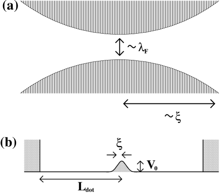
FIG. 1.: (a) Schematic diagram for a single orbital-mode connection between the two dots. Over a distance of order $\xi$, the connection narrows to a minimum width on the order of the Fermi wavelength $\lambda_{\text{F}}$. (b) “Box-like” double-dot system with a central barrier. Hard confining walls are located at a distance $L_{\text{dot}}$ from the barrier. The barrier is characterized by its height $V_{0}$ and half width $\xi$.

frequency of the inverted parabolic well. This frequency is proportional to the square root of the barrier curvature, which is proportional to $V_{0}/\xi^{2}$. It follows that the limit $\xi\rightarrow 0$ corresponds to the limit $U/W\rightarrow 0$. For $\xi\neq 0$, on the other hand, it is not always true that $U/W\ll 1$. In fact, in recent experiments by Waugh et al. [2], Crouch et al. [3], and Livermore et al. [4], it appears that $U/W$ is roughly $1$. Under such circumstances, we find that, for a given small value of the channel conductance ($g\ll 1$), the fractional peak splitting $f$ is larger than the zero-width splitting, $f_{\xi=0}$, by a small but noticeable amount, and, in the extreme limit of $g\rightarrow 0$, the ratio of the finite-width peak splitting to the previously calculated zero-width peak splitting becomes very large. For intermediate values of $g$, on the other hand, the primary effect is a small increase in $f$ accompanied by a reduction of the slope of the $f$-versus-$g$ curve.

To find the leading term in the finite-width fractional peak splitting we adopt a stationary-state approach, [10] in which the first step is to solve for the single-particle eigenstates of non-interacting electrons moving in the electrostatic potential of the coupled dots. The capacitive interactions between the electrons are then expressed in terms of these non-interacting double-dot eigenstates, and the off-diagonal elements of the interactions are treated perturbatively. The leading term in the finite-width fractional peak splitting, $f^{(1)}$, is determined by finding the value for $\rho=1$ of a more general quantity $\tilde{f}^{(1)}(\rho)$, where $\rho$ is a dimensionless parameter (defined by Eq. 2 below) which is a measure of the bias asymmetry between the dots. [5, 6] In the limit $U/W\rightarrow 0$, the zero-width result, $f_{\xi=0}^{(1)}$, is recovered. For finite $U/W$, an approximate analytic calculation demonstrates the limiting $1/|\ln g|$ behavior, which is confirmed by numerical results. For the particular choice $U/W=1$, which corresponds to recent experiments, [2, 3, 4] as well as for various other choices of the ratio $U/W$, the leading term in the fractional peak splitting is computed numerically as a function of $g$. It is confirmed that the condition $\xi\neq 0$ leads to an upward shift of the peak splitting for weakly coupled dots ($g\ll 1$). As $g$ becomes larger, the effect of allowing $\xi\neq 0$ becomes less dramatic, and, for $U/W\simeq 1$, previous predictions for the fractional peak splitting at intermediate values of $g$ are essentially unaltered.

The structure of this paper is as follows. Sec. II develops the stationary-state approach for calculating $\tilde{f}(\rho)$. Sec. III implements this approach for a parabolic interdot barrier, verifying the $1/|\ln g|$ behavior of the $g\rightarrow 0$ peak splitting that arises for $\xi\neq 0$ and putting the finite-width calculation in the context of earlier work. Sec. IV summarizes the results and comments on the possible effects of $\xi\neq 0$ when the dots are strongly coupled ($g\simeq 1$).

II The Stationary-State Approach

In order to solve for $\tilde{f}(\rho)$ via the stationary-state approach, we make the problem one-dimensional by considering a smooth, adiabatic interdot connection [see Fig. 1(a)] which, for simplicity, we presume to contain only one transverse orbital mode that lies near or below the Fermi energy $E_{\text{F}}$. [11] (The use of one orbital mode corresponds to the spin-symmetric $N_{\text{ch}}=2$ experiments of Waugh et al. [2], Crouch et al. [3], and Livermore et al. [4]) For such a single orbital-mode connection, the only parts of an electron wavefunction that can pass from dot to dot are those that overlap with the lowest transverse mode. Hence, in investigating the effect of the interdot connection, we can ignore all electrons but those in this lowest mode. We are left with a one-dimensional problem in which a representative electron with single-particle energy $E$ moves in an effective potential $V(x)=E_{\text{tr}}(x)+V_{\text{el}}(x)$, where $E_{\text{tr}}(x)$ is the spatially dependent energy of the lowest transverse mode and $V_{\text{el}}(x)$ is the spatially dependent electrostatic energy. The characteristic length scale for the spatial variation of the effective potential is the barrier width $\xi$.

After adding hard boundaries at a distance $L_{\text{dot}}$ from the barrier, we have a “box-like” double-dot system with a smoothly varying longitudinal potential [see Fig. 1(b)]. The Hamiltonian consists of two components. The first, $H_{0}$, is a diagonal term giving the energies of the non-interacting, single-particle eigenstates, which form a discrete spectrum with an average level spacing proportional to $\hbar v_{\text{F}}/L_{\text{dot}}$ near the Fermi surface, where $v_{\text{F}}$ is the Fermi velocity. The second, $H_{C}$, gives the capacitive energy cost of moving electrons from one side of the barrier to the other: [5, 6]

$$H_{C}=U(\hat{n}-\rho/2)^{2}\,.$$ (2)

Here, $\hat{n}$ counts the electrons transferred from dot 1 to dot 2 (assuming, for convenience, an even total number of electrons initially divided equally between the two dots). The dimensionless parameter $\rho$ is a measure of the capacitively weighted bias and favors occupation of dot 2 when $\rho>0$. (Note that $U$ equals the quantity $U_{2}$ of previous work. [5, 6])

We need to solve for the dimensionless channel conductance $g$ and the fractional peak splitting $f$. For the non-interacting electrons characterized by $H_{0}$, the dimensionless channel conductance $g$ is simply the transmission probability for a particle incident on the barrier at the Fermi energy $E_{\text{F}}$. [10] $f$ is not so easily determined because, in its evaluation, $H_{C}$ is relevant. Thus, we must develop a means of dealing with $\hat{n}$, which is not diagonal in the basis of non-interacting single-particle eigenstates that is the cornerstone of our approach.

Our strategy is to switch to a basis that is simply related to the eigenstate basis but which renders $\hat{n}$ nearly diagonal at energies that are low compared to the barrier. We use the fact that, for a bound system containing two equal potential minima, the eigenstates come in well-defined, discrete pairs. [12] The states in these pairs have similar energies but opposite parities, the even-parity state having a lower energy than the odd-parity state. Thus, the non-interacting part of the Hamiltonian can be written in the form

$$H_{0}=\sum_{\sigma,j}E_{S}(j)c^{\dagger}_{Sj\sigma}\,c_{Sj\sigma}+\sum_{\sigma,j}E_{A}(j)c^{\dagger}_{Aj\sigma}\,c_{Aj\sigma}\,,$$ (3)

where $S$ and $A$ are the even and odd parity indices, $j$ is the pair index, and $\sigma$ is the spin index (which might be more generally regarded as a channel index).

At lower and lower energies relative to the barrier, the splitting within the pairs, $|E_{A}(j)-E_{S}(j)|$, approaches zero, but the spacing between pairs, $|E_{S}(j+1)-E_{A}(j)|$, remains approximately equal to $\delta$, where $\delta=\pi\hbar v_{\text{F}}/L_{\text{dot}}$ (assuming we do not stray too far from the Fermi surface). It follows that, at low energies, one can form doublets of quasi-localized states—states that lie mostly on one of the two sides of the central barrier—from linear combinations of the symmetric and antisymmetric components of each eigenstate pair. [12] If $\phi_{Sj}(x)$ and $\phi_{Aj}(x)$ are the symmetric and antisymmetric eigenfunctions of the $j$th lowest-energy pair (with appropriately chosen overall phases), the recipe for the quasi-localized wavefunctions is

$$\Omega_{j\alpha}(x)=\frac{1}{\sqrt{2}}\left[\phi_{Sj}(x)+(-1)^{\alpha+1}\phi_{Aj}(x)\right],$$ (4)

where the dot index $\alpha$ signifies that $\Omega_{j\alpha}(x)$ is primarily localized on the dot 1 side of the barrier if $\alpha=1$ and on the dot 2 side if $\alpha=2$.

At high energies relative to the barrier, we cannot form quasi-localized wavefunctions from combinations of just two states. Nevertheless, we continue to form the linear combinations analogous to those of Eq. 4. We refer to the full set of states $\Omega_{j\alpha}(x)$ as semi-localized to indicate that these states are sometimes quasi-localized (i.e., when they lie at low energies relative to the interdot barrier) and sometimes not.

The semi-localized states constitute the complete and orthogonal basis that we need to render $\hat{n}$ nearly diagonal at low energies. Their simple relation to the double-dot eigenstates translates into an equally simple relation between the corresponding creation and annihilation operators. The semi-localized annihilation operators are given by

$$a_{j\alpha\sigma}=\frac{1}{\sqrt{2}}\left[c_{Sj\sigma}+(-1)^{\alpha+1}c_{Aj\sigma}\right]\,,$$ (5)

and the corresponding expression for $H_{0}$ is

$$H_{0}=\sum_{\sigma,\alpha,j}E(j)a^{\dagger}_{j\alpha\sigma}a_{j\alpha\sigma}-\sum_{\sigma,j}t(j)(a^{\dagger}_{j2\sigma}a_{j1\sigma}+\text{H.c.})\,,$$ (6)

where $E(j)$ is the average energy of the pair and $t(j)$ is half the energy difference within the pair:

$$E(j) = \frac{E_{A}(j)+E_{S}(j)}{2}\,,$$ (7)

$$t(j) = \frac{E_{A}(j)-E_{S}(j)}{2}\,.$$ (8)

It is important to note that, whereas $E(j)$ is in general on the order of the Fermi energy, $t(j)$ is no greater than the average level spacing $\delta=\pi\hbar v_{\text{F}}/L_{\text{dot}}$ and becomes vanishingly small in the large-dot limit ($L_{\text{dot}}\rightarrow\infty$). The minuteness of $t(j)$ will permit us to ignore it in calculating the leading contribution to the fractional peak splitting.

We now write $\hat{n}$ in terms of the semi-localized operators. If dot 1 corresponds to the $x<0$ side of the barrier and dot 2 corresponds to the $x>0$ side, we have

$$\hat{n}=\frac{1}{2}\int\!dx\left[\Theta(x)-\Theta(-x)\right]\psi^{\dagger}(x)\psi(x),$$ (9)

where $\psi(x)$ is the position operator and $\Theta(x)$ is the Heaviside step function. [13]

After writing $\psi(x)$ in terms of the semi-localized operators $a_{j\alpha\sigma}$, we see that $\hat{n}=\hat{n}_{0}+\delta\hat{n}_{\text{C}}+\delta\hat{n}_{\text{T}}$, where $\hat{n}_{0}$ corresponds to the $\hat{n}$ we would have if the semi-localized states were truly localized, $\delta\hat{n}_{\text{C}}$ is the part of $\delta\hat{n}=(\hat{n}-\hat{n}_{0})$ that does not transfer electrons from dot 1 to dot 2, and $\delta\hat{n}_{\text{T}}$ is the part of $\delta\hat{n}$ that does effect such a transfer:

$$\hat{n}_{0} = \sum_{\sigma,\alpha,j}\frac{(-1)^{\alpha}}{2}a^{\dagger}_{j\alpha\sigma}a_{j\alpha\sigma},$$ (10)

$$\delta\hat{n}_{\text{C}} = \sum_{\sigma,\alpha,j_{1},j_{2}}\left[B(j_{2},\alpha;j_{1},\alpha)-\frac{(-1)^{\alpha}}{2}\delta_{j_{1},j_{2}}\right]a^{\dagger}_{j_{2}\alpha\sigma}a_{j_{1}\alpha\sigma},$$ (11)

$$\delta\hat{n}_{T} = \sum_{\sigma,\alpha,j_{1},j_{2}}B(j_{2},\bar{\alpha};j_{1},\alpha)a^{\dagger}_{j_{2}\bar{\alpha}\sigma}a_{j_{1}\alpha\sigma}\,.$$ (12)

Here, $\bar{\alpha}$ means “not $\alpha$” and

$$B(j_{2},\alpha_{2};j_{1},\alpha_{1}) = \frac{1}{2}\int_{0}^{L_{\text{dot}}}\!dx\,\,\left[(-1)^{\alpha_{1}+1}\phi^{*}_{Sj_{2}}(x)\,\phi_{Aj_{1}}(x)\right.$$ (14)

$$\hskip 7.22743pt\left.\mbox{}+(-1)^{\alpha_{2}+1}\phi^{*}_{Aj_{2}}(x)\,\phi_{Sj_{1}}(x)\right].$$

We have obtained the desired “semi-diagonal” form of $\hat{n}$. Using $\delta\hat{n}=\delta\hat{n}_{\text{C}}+\delta\hat{n}_{\text{T}}$ and assuming that $g$ is small, we express the Hamiltonian in terms of one non-perturbative piece, $H^{\prime}_{0}$, and two perturbative pieces, $H^{\prime}_{\text{T}}$ and $H^{\prime}_{\text{C}}$:

$$H^{\prime}_{0} = \sum_{\sigma,\alpha,j}E(j)a^{\dagger}_{j\alpha\sigma}a_{j\alpha\sigma}+U(\hat{n}_{0}-\rho/2)^{2},$$ (15)

$$H^{\prime}_{\text{T}} = -\sum_{\sigma,j}t(j)(a^{\dagger}_{j2\sigma}a_{j1\sigma}+\text{H.c.}),$$ (16)

$$H^{\prime}_{\text{C}} = U(\hat{n}_{0}-\rho/2)\delta\hat{n}+U\delta\hat{n}(\hat{n}_{0}-\rho/2)+U(\delta\hat{n})^{2}.$$ (17)

As in Refs. 5 and 6, the fractional peak splitting is determined from $\tilde{f}(\rho)$, where

$$\tilde{f}(\rho)=\frac{\Delta(0)-\Delta(\rho)}{U/4}$$ (18)

and $\Delta(\rho)$ is the energy shift of the ground state of $H^{\prime}_{0}$ due to the perturbations $H^{\prime}_{\text{T}}$ and $H^{\prime}_{\text{C}}$ for the given value of $\rho$, where $0\leq\rho<1$ and the total number of particles in the double-dot system is even. The quantity $\left[\lim_{\rho\rightarrow 1}\tilde{f}(\rho)\right]$ equals the fractional peak splitting $f$.

Eq. 18 tells us that we are only interested in relative energy shifts. Consequently, we can ignore terms such as $\langle 0|U(\delta\hat{n})^{2}|0\rangle$ that are independent of $\rho$. (Here the brackets indicate an expectation value taken in the ground state of $H^{\prime}_{0}$.) Another set of irrevelant terms are those of the form $\langle 0|U(\hat{n}_{0}-\rho/2)\delta\hat{n}|0\rangle$, which are zero due to the symmetry of the ground state with respect to interchange of the two dots. Finally, terms that contain $H^{\prime}_{\text{T}}$ are also negligible because $t(j)$ goes to zero with the reciprocal of the system size and, unlike $\delta\hat{n}$, $H^{\prime}_{\text{T}}$ only connects each state to one other, rather than connecting each state to a manifold of others (see Ref. 5 for a similar situation with regard to odd orders in the transfer-Hamiltonian perturbation theory). After the above terms are omitted, it is apparent that the leading perturbative energy shift comes from the term that is second order in $H^{\prime}_{\text{C}}$. To lowest order in $\delta\hat{n}$, this term is

$$\Delta^{(2)}(\rho)=-U^{2}\left\langle 0\left|\delta\hat{n}\,P_{0}\frac{(\hat{n}_{0}-\rho)^{2}}{H^{\prime}_{0}-E^{\prime}_{0}(\rho)}P_{0}\,\delta\hat{n}\right|0\right\rangle,$$ (19)

where $E^{\prime}_{0}(\rho)$ is the energy of the ground state of $H^{\prime}_{0}$ and where $P_{0}$ is the operator that projects out the unperturbed ground state. $\Delta^{(2)}(\rho)$ can easily be seen to consist of two distinct parts: a term second-order in $\delta\hat{n}_{C}$, which involves hopping between states semi-localized on the same dot, and a term second-order in $\delta\hat{n}_{T}$, which involves hopping between states on different dots.

With Eq. 19, we have completed our tour of how to use the stationary-state approach to find both the interdot channel conductance $g$ and the fractional peak splitting $f$. In order to progress further, we must adopt a model for the barrier that gives the energy dependence of the elements of $\delta\hat{n}$ (recall Eqs. 12 and 14).

III Peak Splitting and Conductance for a Parabolic Barrier

We assume that the barrier in the interdot tunneling channel can be reasonably modeled by a parabolic one. For an energy barrier with peak height $V_{0}$, such a model is plausible when $V_{0}\simeq E_{\text{F}}\gg U$, which is the regime of experimental interest. [14] The formula for a parabolic potential $V(x)$ centered at the origin with half width $\xi$ is the following:

$$V(x)=\left\{\begin{array}[]{ll}V_{0}\left(1-\frac{x^{2}}{2\xi^{2}}\right)&\mbox{if $|x|<\sqrt{2}\xi$}\\ 0&\mbox{otherwise.}\end{array}\right.$$ (20)

A crucial energy scale for this barrier is the harmonic oscillator frequency $\omega$ of the inverted parabolic well. This frequency is given by the formula

$$\hbar\omega=\left(\frac{1}{\pi\sqrt{2}}\right)\frac{(2\pi\hbar)^{2}}{2m\lambda_{V}\xi}\,,$$ (21)

where $2\pi/\lambda_{V}=\sqrt{2mV_{0}/\hbar^{2}}$ and $m$ is the effective mass of the electron.

The problem of transmission through and reflection from a parabolic barrier is well known and exactly solvable. [15, 16] The solutions are parabolic cylinder functions, [17] and the dimensionless channel conductance is given by [16, 18]

$$g=\frac{1}{1+e^{-2\pi y(E_{\text{F}})}}\,,$$ (22)

where $E_{\text{F}}$ is the Fermi energy and

$$y(E)=\frac{E-V_{0}}{\hbar\omega}\,.$$ (23)

From these equations, it follows that

$$\frac{(V_{0}-E_{\text{F}})}{\hbar\omega}=\frac{1}{2\pi}\ln\left(\frac{1-g}{g}\right)\,,$$ (24)

and, for $g\ll 1$,

$$\frac{(V_{0}-E_{\text{F}})}{V_{0}}\simeq\frac{1}{2\pi^{2}\sqrt{2}}\left(\frac{\lambda_{\text{V}}}{\xi}\right)|\ln g|\,.$$ (25)

Eq. 25 tells us that, even for experimental systems [2, 3] in which $\xi$ is quite small ($\xi\simeq\lambda_{\text{F}}$), $E_{\text{F}}$ is close to $V_{0}$ for $|\ln g|\ll 2\pi^{2}\sqrt{2}$. Thus, the assumption of a parabolic barrier appears reasonable for any measurable value of the interdot conductance.

We now consider the sizes of the various energies that appear in our peak splitting calculations. Equation 22 indicates that the energy scale $W$ for the variation of transmission probabilities is $\hbar\omega/2\pi$. Recalling our discussion in Sec. I, we have

$$\frac{U}{W}=\frac{2\pi U}{\hbar\omega}\,.$$ (26)

As observed in previous work, [3, 5] for symmetric dots, $U$ equals $e^{2}/(C_{\Sigma}+2C_{\text{int}})$, where $C_{\Sigma}$ is the total capacitance of one of the two dots and $C_{\text{int}}$ is the interdot capacitance. The energy scale $\hbar\omega$ is, by comparison, only roughly known. From the fact that the barrier height $V_{0}$ is approximately equal to $E_{\text{F}}$, we know that $\lambda_{V}\simeq\lambda_{\text{F}}$. For $\xi$, we can use the “device resolution” $d$, which is the distance between the surface metallic gates and the two-dimensional electron gas (2DEG) and is typically on the order of $100~{}\text{nm}$. The fact that the approximation $\xi\simeq d$ should be accurate safely within a factor of $2$ can be surmised from calculations such as that of Davies and Nixon [19] in which they show that the potential profile induced in a 2DEG by a narrow line gate has a half width at half maximum that is approximately equal to $d$. [20, 21] In the AlGaAs/GaAs heterostructures of Waugh et al., Crouch et al., and Livermore et al., [2, 3, 4] where $d$ is fairly small, about $50$ nm (approximately one Fermi wavelength), further circumstantial evidence for $\xi\simeq d$ comes from the fact that the space between the gates that form the interdot barrier is about $100$ nm (see Ref. 5). It follows that, for these experimental systems, $\hbar\omega$ is approximately $0.2E_{\text{F}}$. On the other hand, $U$ is about $0.03E_{\text{F}}$, and, therefore, to within a factor of $2$, $2\pi U/\hbar\omega\simeq 1$. For different systems in which the Fermi wavelength is still about $50$ nm but the gates are further from the 2DEG, [22] the ratio $2\pi U/\hbar\omega$ is presumably even larger. Consequently, we expect it to be quite generally true that the ratio $U/W=2\pi U/\hbar\omega$ is greater than or approximately equal to $1$.

On the other hand, since, in the sorts of experimental situations with which we are primarily concerned, [2, 3, 4] both $W/E_{\text{F}}$ and $U/E_{\text{F}}$ are much less than $1$, we are justified in linearizing the single-particle energy spectrum about the Fermi surface, taking $E(j)=E_{\text{F}}+\hbar v_{\text{F}}[k(j)-k_{\text{F}}]$, where $k(j)=\sqrt{2mE(j)/\hbar^{2}}$.

We must now calculate $\left|B(j_{2},\alpha_{2};j_{1},\alpha_{1})\right|$ when $j_{1}\neq j_{2}$. We avail ourselves of the exact, real solutions for the wavefunctions $\phi_{Pj}(x)$ in the presence of a parabolic potential [16, 17] ($P$ is the parity index, which we set equal to $0$ for symmetric wavefunctions and $1$ for antisymmetric wavefunctions). Connecting these to the corresponding sinusoids, we find that, for $x>\sqrt{2}\xi$ and $L_{\text{dot}}\gg\xi$, the eigenfunctions are approximately given by

$$\phi_{Pj}(x)=\frac{(-1)^{P}}{\sqrt{L_{\text{dot}}}}\cos[k(y_{Pj})(x-\sqrt{2}\xi)+\gamma_{P}(y_{Pj})],$$ (27)

where $y_{Pj}=y(E_{Pj})$ and $k(y_{Pj})=\sqrt{2mE_{P}(j)/\hbar^{2}}$. The hard-wall boundary condition then demands that there be an integer $n$ such that the quantity in brackets equals $(2n+1)\pi/2$ when $x=L_{\text{dot}}$.

As for the phase $\gamma_{P}(y)$ itself, it can be written in the following general form:

$$\gamma_{P}(y)=(-1)^{P}R(y)+D(y)\,,$$ (28)

If the connection to the sinusoids is made using the leading large-$x$ forms for the parabolic cylinder functions, [16, 17] $R(y)$ and $D(y)$ are given by

$$R(y) = \frac{1}{2}\arctan(e^{\pi y})\,,$$ (29)

$$D(y) = \frac{1}{2}[\arg\Gamma(1/2-iy)+y\ln(4\pi\sqrt{2}\xi/\lambda_{V})]+D_{0}\,,$$ (30)

where $D_{0}$ is independent of $y$.

Returning to Eq. 14, we find that, if we restrict the integral to $x>\sqrt{2}\xi$, we have

$$B^{\prime} \simeq (-1)^{\alpha+1}\,\frac{\sin[D(y_{2})-D(y_{1})]\,\cos[R(y_{2})+R(y_{1})]}{2(k_{2}-k_{1})L_{\text{dot}}}\,,$$ (31)

$$\bar{B}^{\prime} \simeq (-1)^{\alpha+1}\,\frac{\cos[D(y_{2})-D(y_{1})]\,\sin[R(y_{2})+R(y_{1})]}{2(k_{2}-k_{1})L_{\text{dot}}}\,,$$ (32)

where the bar of $\bar{B}^{\prime}$ indicates that this is the term that moves electrons from dot $\alpha$ to dot $\bar{\alpha}$ and we have anticipated a continuum limit in replacing $y_{Pj}$ and $k(y_{Pj})$ by $y_{j}=y[E(j)]$ and $k_{i}=k(y_{j})$.

In the calculation of $\bar{B}^{\prime}$ and $B^{\prime}$, we have neglected the integration over the region $|x|<\sqrt{2}\xi$. The results can therefore be expected to involve errors of order $\xi/L_{\text{dot}}$ when compared to the actual values of $B$ and $\bar{B}$. For $\bar{B}^{\prime}$, this is not too much of a concern since, when both $k_{2}$ and $k_{1}$ approach the Fermi energy, the numerator of $\bar{B}^{\prime}$ goes to $\sqrt{g}$ and the denominator goes to zero. Thus, for non-infinitesimal $g$, if we restrict our wave-vectors to a range about the Fermi surface such that $|k_{i}-k_{F}|\ll 1/\xi$ (in which case $\cos[D(y_{2})-D(y_{1})]$ can be approximated by $1$), corrections to $\bar{B}^{\prime}$ should be relatively small.

In contrast, the term $B^{\prime}$ is a bit more problematic, for its numerator goes to zero as $(k_{2}-k_{1})\xi$. Consequently, near the Fermi surface this term is of the order of the error, and to obtain a reliable result we must complete the integral numerically, using the parabolic cylinder functions in place of our sinusoids when $|x|<\sqrt{2}\xi$. We then find that the form for $B^{\prime}$ approximates the magnitude of the actual value of $B$ if, after approximating $\cos[R(y_{2})+R(y_{1})]$ by $1$, we replace $[D(y_{2})-D(y_{1})]$ with $\kappa(y_{2}-y_{1})$, where $\kappa\simeq 0.1$ for $g\sim 0.1$ and $\kappa\rightarrow 0$ as $g\rightarrow 0$. Our conclusion is that

$$B \simeq (-1)^{\alpha+1}\,\frac{\sin[\kappa(y_{2}-y_{1})]}{2(k_{2}-k_{1})L_{\text{dot}}}\,,$$ (33)

$$\bar{B} \simeq (-1)^{\alpha+1}\,\frac{\sin[R(y_{2})+R(y_{1})]}{2(k_{2}-k_{1})L_{\text{dot}}}\,.$$ (34)

We can now calculate the leading parts of the energy shift $\Delta(\rho)$. The contribution from hopping between states on the same dot is given approximately by

$$\Delta_{C}^{(2)}(\rho) \simeq -\left(\frac{U\rho^{2}}{4}\right)\frac{N_{\text{ch}}}{\pi^{3}}\left(\frac{2\pi U}{\hbar\omega}\right)$$ (36)

$$\hskip 21.68121pt\times\int_{-Y_{1}}^{0}\!dy_{1}\!\int_{0}^{Y_{2}}\!dy_{2}\,\frac{\sin^{2}[\kappa(y_{2}-y_{1})]}{(y_{2}-y_{1})^{3}}\,,$$

where the $y_{i}$’s are now measured relative to $y_{\text{F}}$ (i.e., $y_{i}\rightarrow y_{i}+y_{\text{F}}$). The contribution from hopping between the dots obeys

$$\Delta_{T}^{(2)}(\rho) = -\frac{N_{\text{ch}}U^{2}}{4}\int_{-\Lambda_{3}}^{0}\!\frac{dk_{1}}{\pi}\!\int_{0}^{\Lambda_{4}}\!\frac{dk_{2}}{\pi}\,$$ (40)

$$\hskip 14.45377pt\times\frac{\sin^{2}[\tilde{R}(\hbar v_{\text{F}}k_{2}/\hbar\omega)+\tilde{R}(\hbar v_{\text{F}}k_{1}/\hbar\omega)]}{(k_{2}-k_{1})^{2}}$$

$$\hskip 14.45377pt\times\left\{\frac{(1-\rho)^{2}}{\hbar v_{F}(k_{2}-k_{1})+U(1-\rho)}\,\right.$$

$$\hskip 43.36243pt\left.+\,[\rho\rightarrow-\rho]\right\}\,,$$

where $\tilde{R}(y)=R[y(E_{\text{F}})+y]$ and the bracketed expression $\rho\rightarrow-\rho$ stands for the quantity obtained by replacing $\rho$ by $-\rho$ in the previous term. In Eqs. 36 and 40, ultraviolet cutoffs $Y_{r}$ and $\Lambda_{r}$ have been inserted in recognition of the fact that our formulas for the integrands break down at some distance $Y_{r}$ or $\Lambda_{r}$ from the Fermi surface.

For the same-dot-hopping shift $\Delta_{C}^{(2)}$, the presence of such cutoffs is essentially irrelevant since we find this term to be effectively negligible no matter what the choice of $Y_{r}$. In particular, even when the cutoffs are taken to infinity, this segment of the energy shift produces a contribution to $\tilde{f}(\rho)$ (recall Eq. 18) that is bounded by the following formula:

$$\tilde{f}_{C}(\rho)\lesssim\frac{N_{\text{ch}}\rho^{2}}{200}\left(\frac{2\pi U}{\hbar\omega}\right)\,.$$ (41)

The real contribution is perhaps substantially smaller than the bound because the integrand of Eq. 36 is systematically too large for the infinitesimal-transmission states that correspond to $|y_{1}|\gtrsim 1$.

In any case, it is clear that the contribution to $\tilde{f}(\rho)$ from same-dot hopping is essentially negligible. For $N_{\text{ch}}\lesssim 2$ and $(2\pi U/\hbar\omega)\ll 10$, $\tilde{f}_{C}(\rho)$ is extremely small and essentially constant in $g$. Under such circumstances, it does not significantly affect even the quantitative results. When $(2\pi U/\hbar\omega)\gtrsim 10$, on the other hand, it can be relatively large. Nevertheless, it remains unimportant, for in this regime we can only obtain qualitatively good results for the value of $\Delta_{T}^{(2)}(\rho)$, and, qualitatively, the upward shift of $\tilde{f}(\rho)$ induced by same-dot hopping merely reinforces the effect from hopping between the dots.

We now consider the cutoffs $\Lambda_{r}$ and their impact upon our understanding of the interdot-hopping result. Since the integrand in Eq. 40 is reliably precise only when $k_{1}$ and $k_{2}$ are within $1/\xi$ of $k_{\text{F}}$, the ultraviolet cutoffs should be chosen such that $\Lambda_{r}\sim 1/\xi$. It follows that, to capture with quantitative precision the leading behavior of the peak splitting for $g\ll 1$, the set of wave-vectors within $1/\xi$ of the Fermi surface should encompass the range of energies in which the quantity $\tilde{R}(E)$ is rapidly growing. Consequently, the set of wave-vectors must extend at least to $k_{\text{F}}+k_{0}$, where $E(k_{\text{F}}+k_{0})=V_{0}$. From Eq. 24, we see that the identity $k_{0}=(V_{0}-E_{\text{F}})/\hbar v_{\text{F}}$ yields

$$k_{0}\xi\simeq\frac{1}{2\pi\sqrt{2}}\ln\!\left(\frac{1-g}{g}\right)\,.$$ (42)

If we require that $k_{0}\xi\lesssim 1$, we see that, for $g\ll 1$, we must have $|\ln g|\lesssim 2\pi\sqrt{2}$. Thus, we have a lower bound on the values of $g$ for which our approximations are reliable. Fortunately, the lower bound is very small, and the requirement is only that $g\gtrsim 10^{-4}$.

We are now prepared to calculate $\Delta_{T}^{(2)}(\rho)$. After a switch to the dimensionless variables $x_{r}=(-1)^{r}\hbar v_{\text{F}}k_{r}/U$, Eq. 40 reduces to

$$\Delta_{T}^{(2)}(\rho) \cong -\frac{N_{\text{ch}}U}{4\pi^{2}}\int_{0}^{\bar{\chi}_{1}}\!dx_{1}\!\int_{0}^{\bar{\chi}_{2}}\!dx_{2}\,\frac{\tilde{T}(x_{1},x_{2})}{x_{2}+x_{1}+1-\rho}\mbox{}\,$$ (44)

$$\hskip 14.45377pt+\,[\rho\rightarrow-\rho]\,,$$

where $\bar{\chi}_{r}=\hbar v_{\text{F}}\Lambda_{r}/U$, the symbol $\,\cong\,$ signifies equality modulo terms that are independent of $\rho$, and the quantity $\tilde{T}(x_{1},x_{2})$ is given by

$$\tilde{T}(x_{1},x_{2})=\sin^{2}[\tilde{R}(Ux_{2}/\hbar\omega)+\tilde{R}(-Ux_{1}/\hbar\omega)]\,.$$ (45)

To obtain a result with negligible dependence on the cutoffs $\bar{\chi}_{r}$, we must have $\bar{\chi}_{r}\gg 1$. On the other hand, to ensure that the answer is quantitatively reliable, we need $\Lambda_{r}\lesssim 1/\xi$ or, equivalently, $\bar{\chi}_{r}\lesssim\hbar v_{\text{F}}/U\xi$. Thus, as promised, we can only expect Eq. 44 to give quantitatively reliable results for $U\ll\hbar v_{\text{F}}/\xi$; i.e., for $2\pi U/\hbar\omega\ll 2\pi\sqrt{2}$, where $2\pi\sqrt{2}\simeq 9$.

Having dealt with the issue of the ultraviolet cutoffs, we can now go about the business of evaluating the right side of Eq. 44. From the identity $\tilde{T}(0,0)=g$, it follows that the limit $2\pi U/\hbar\omega\rightarrow 0$ yields the zero-width ($\xi=0$) linear-in-$g$ equation for $\Delta^{(2)}(\rho)$ that was previously derived via a transfer-Hamiltonian approach. [5, 6, 8, 9] In contrast, in the limit $2\pi U/\hbar\omega\rightarrow\infty$, the energy shift given by Eq. 44 is independent of the interdot conductance for $g$ a finite distance from both $0$ and $1$. The constancy of the shift follows from the fact that, except when $g$ equals $0$ or $1$, $\tilde{T}(x_{1},x_{2})$ is always $0.5$ within the bounds of integration, and the relevant parts of the energy shift are therefore the same as for $(2\pi U/\hbar\omega)=0$ and $g=0.5$. It should be re-emphasized, however, that such a result for the limit $2\pi U/\hbar\omega\rightarrow\infty$ can only be expected to be qualitatively correct.

What happens when the barrier width $\xi$ is between $0$ and $\infty$? By performing two partial integrations of the righthand side of Eq. 44 and dropping terms that go to zero as the cutoffs $\Lambda_{r}$ become infinite, we find that

$$\tilde{f}^{(1)}(\rho) = \frac{N_{\text{ch}}g}{\pi^{2}}\,(1-\rho)\ln(1-\rho)$$ (50)

$$\hskip 7.22743pt\mbox{}+\frac{N_{\text{ch}}}{\pi^{2}}\left\{\int_{0}^{\bar{\chi}_{1}}\!dx_{1}\!\left[\frac{\partial\tilde{T}(x_{1},0)}{\partial x_{1}}\,h(\rho,x_{1},0)\right]\right.$$

$$\hskip 7.22743pt\mbox{}+\int_{0}^{\bar{\chi}_{2}}\!dx_{2}\!\left[\frac{\partial\tilde{T}(0,x_{2})}{\partial x_{2}}\,h(\rho,0,x_{2})\right]$$

$$\hskip 7.22743pt\mbox{}\left.+\int_{0}^{\bar{\chi}_{1}}\!dx_{1}\!\int_{0}^{\bar{\chi}_{2}}\!dx_{2}\,\frac{\partial^{2}\tilde{T}(x_{1},x_{2})}{\partial x_{1}\partial x_{2}}\,h(\rho,x_{1},x_{2})\right\}$$

$$\mbox{}\,+\,[\rho\rightarrow-\rho]\,,$$

where $h(\rho,x_{1},x_{2})=(x_{2}+x_{1}+1-\rho)\ln(x_{2}+x_{1}+1-\rho)$. The first term on the righthand side of Eq. 50 is the zero-width result. The other terms, which go to zero in the limit $\xi\rightarrow 0$, are the corrections due to a nonzero width.

Numerical evaluations of Eq. 50 are plotted in Fig. 2(a) for several values of the parameter $2\pi U/\hbar\omega$ in addition to the analytically derived results for the limits of zero-width and infinite-width barriers. A curious feature of these curves is that the corrections to the zero-width behavior are antisymmetric about $g=0.5$, a property that can be demonstrated by considering what happens to the integrands under the transformations $g\!\leftrightarrow\!(1-g)$ and $x_{1}\!\leftrightarrow\!x_{2}$. Though the antisymmetry is suggestive, it must be remembered that $\tilde{f}^{(1)}(\rho)$ is only the leading term in a perturbative expansion about $g=0$. The small positive contribution to $\tilde{f}(\rho)$ that comes from the formula for the same-dot-hopping shift $\Delta_{C}^{(2)}$ breaks this antisymmetry, and other higher-order corrections are likely to do the same. Nevertheless, some sort of rough antisymmetry about $g=0.5$ is probably preserved, for, just as we find that, at small $g$, $\tilde{f}(\rho)$ is enhanced by hopping connections to states with large transmission amplitudes, so we can expect that, at large $g$, $\tilde{f}(\rho)$ is diminished by the fact that many of the occupied states from which one hops have transmission probabilities that are less than $g$.

Such musings aside, we can gain further insight into the nature of our result for $\tilde{f}^{(1)}(\rho)$ by making a rough analytic approximation to the righthand side of Eq. 50. To do this, it is best to return to Eqs. 18 and 44 and to derive the equivalent expression

$$\tilde{f}^{(1)}(\rho) = \frac{2N_{\text{ch}}\rho^{2}}{\pi^{2}}\int_{0}^{\bar{\chi}_{1}}\!dx_{1}\!\int_{0}^{\bar{\chi}_{2}}\!dx_{2}\frac{\tilde{T}(x_{1},x_{2})}{(x_{2}+x_{1}+1)}$$ (52)

$$\hskip 14.45377pt\times\frac{1}{(x_{2}+x_{1}+1-\rho)(x_{2}+x_{1}+1+\rho)}.$$

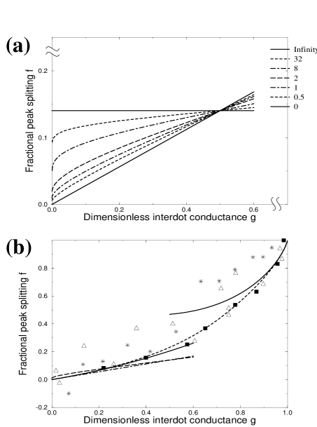
FIG. 2.: (a) Plots of the leading $g\rightarrow 0$ term of $f$, the fractional peak splitting, as a function of $g$, the dimensionless interdot channel conductance. Each curve corresponds to a different value of the quantity $2\pi U/\hbar\omega$ (see legend on right). All curves are for the case of two interdot tunneling channels, $N_{\text{ch}}=2$. The upward sloping solid line is the linear-in-$g$ result that comes from considering an interdot barrier of effectively zero width ($2\pi U/\hbar\omega=0$). The dashed and dot-dashed curves show the $f$-versus-$g$ dependence for finite-width barriers with $2\pi U/\hbar\omega$ taking on values from $0.5$ to $32$. The horizontal solid line gives the leading term in the fractional peak splitting for an infinite-width barrier ($2\pi U/\hbar\omega\rightarrow\infty$). The curves can only be expected to be quantitatively accurate when $2\pi U/\hbar\omega\ll 10$. (b) $f$-versus-$g$ results for the full domain of $g$ when $N_{\text{ch}}=2$. The solid lines are the complete zero-width results in the weak and strong-coupling limits. These results contain both leading and subleading terms.⁶ The plot for the leading zero-width term in the weak-coupling limit ($g\rightarrow 0$) is included as a dot-dashed curve. The small-dashed curve that extends from $(g,f)=(0,0)$ to $(g,f)=(1,1)$ is an interpolating curve that is derived from the zero-width results. The long-dashed line is the $2\pi U/\hbar\omega=1$ curve from Fig. 2(a). The stars, triangles, and squares symbolize different sets of experimental data,^2,4 the squares being the most recent.⁴

We then postulate that, for small $g$, the magnitude of the $\tilde{f}^{(1)}(\rho)$ is largely determined by the portion of the integral that corresponds to $x_{2}\geq x_{0}$, where $x_{0}=\hbar v_{\text{F}}k_{0}/U$ (recall $k_{0}$ from Eq. 42). For $x_{2}$ in this range, $\tilde{T}(x_{1},x_{2})$ is on the order of $1$ and therefore much larger than $\tilde{T}(0,0)$ when $g\ll 1$. We label this high-energy portion of the double integral as $\tilde{f}^{(1)}_{\text{hep}}(\rho)$. Since, in this part of the integral, $\tilde{T}(x_{1},x_{2})$ varies relatively slowly between $0.15$ and $0.5$, we approximate it by a constant $C_{\tilde{T}}$, where we take $C_{\tilde{T}}=0.25$. For $x_{0}\gtrsim 1$, we can drop the $\rho$’s that appear in the integrand of Eq. 52. We then obtain

$$\tilde{f}^{(1)}_{\text{hep}}(\rho)\sim\frac{N_{\text{ch}}\rho^{2}}{4\pi^{2}(x_{0}+1)}\,.$$ (53)

From the identities $f=\tilde{f}(1)$ and $x_{0}=(\hbar\omega/2\pi U)\ln[(1-g)/g]$, we conclude that

$$f^{(1)}_{\text{hep}}\sim\left(\frac{N_{\text{ch}}}{4\pi^{2}}\right)\frac{2\pi U/\hbar\omega}{|\ln g|+2\pi U/\hbar\omega}\,.$$ (54)

This rough approximation to the leading behavior of the fractional peak splitting is only valid when $x_{0}\gtrsim 1$ and $k_{0}\lesssim 1/\xi$. The condition on $x_{0}$ is necessary to justify dropping the $\rho$’s from the integrand in the high-energy portion of the double integral. The condition on $k_{0}$ validates the approximate values for the magnitudes of $|A(j_{2},\alpha_{2};j_{1},\alpha_{1})|$ that we use throughout our calculation. The two restrictions together mean that the range of reliability for our approximation to $\tilde{f}^{(1)}_{\text{hep}}$ is given by

$$\frac{2\pi U}{\hbar\omega}\lesssim|\ln g|\lesssim 2\pi\sqrt{2}.$$ (55)

For $2\pi U/\hbar\omega\simeq 1$, our approximations are good for $g$ between a couple tenths and a few ten-thousandths.

It is instructive to compare our result for $f^{(1)}_{\text{hep}}$ with the zero-width fractional peak splitting, $f^{(1)}_{\xi=0}$. From Eqs. 1 and 54, we see that, for $2\pi U/\hbar\omega=1$, the ratio $f^{(1)}_{\text{hep}}/f^{(1)}_{\xi=0}$ is about $0.6$ when $g=0.1$ and about $25$ when $g=0.001$. For very weak coupling ($g\ll 0.1$), the correction to the $\xi=0$ result is proportionately very large, and, as $g\rightarrow 0$, it dominates the behavior of the peak splitting. On the other hand, as $g$ assumes more intermediate values ($g\sim 0.1$), the results for $\xi=0$ and $\xi\neq 0$ converge.

A direct comparison of our results for $f^{(1)}_{\text{hep}}$ with the full numerical results for $f^{(1)}$, which are plotted in Fig. 2(a), confirms that $f^{(1)}_{\text{hep}}$ does indeed capture the essential $f$-versus-$g$ behavior, particularly as $2\pi U/\hbar\omega$ becomes larger and the exponential enhancement of the tunneling amplitudes becomes more important. The sharp increase in slope as $g\rightarrow 0$ can now be understood as resulting from the fact that, in this limit, the high-energy portion of the peak splitting is proportional to $(2\pi U/\hbar\omega)/|\ln g|$. This proportionality also explains why the increase in slope as $g\rightarrow 0$ becomes less dramatic as $2\pi U/\hbar\omega$ decreases. The success of our rough analytic approximation supports the supposition that, for small $g$, a substantial portion of the peak splitting comes from tunneling into virtual states lying near or above the top of the barrier.

Turning to Fig. 2(b), we now examine the significance of the calculated finite-width corrections in the context of what we know about the $f$-versus-$g$ curve in the entire range from $g=0$ to $g=1$, and we consider the implications of these corrections for the relevant experiments. [2, 3, 4] The long-dashed curve in Fig. 2(b) is the curve from Fig. 2(a) for the value $2\pi U/\hbar\omega=1$, which we believe to be appropriate for the cited experiments. The dot-dashed line is the leading-order-in-$g$, zero-width curve, which also appears in Fig. 2(a). The small-dashed curve in Fig. 2(b) is an interpolation for the entire zero-width $f$-versus-$g$ curve. This interpolation has been designed to match both the second-order-in-$g$ calculation of the fractional peak splitting for weak coupling ($g\simeq 0$) and also the two-term calculation for strong coupling ($g\simeq 1$), which were obtained in Ref. 6 and are shown as solid curves in Fig. 2(b). The stars, triangles, and squares represent different sets of experimental data.

For the particular value of $2\pi U/\hbar\omega$ that is illustrated in Fig. 2(b), we see that, although the finite-width correction to $f$ changes the answer by a large factor in the region of small $g$, the correction is small on an absolute scale. The difference between the dashed curve and the dot-dashed curve never exceeds 0.02 and therefore causes only a small correction to the overall shape of the $f$-versus-$g$ curve. Qualitatively, the correction due to the finite thickness of the barrier is quite similar to adding a small constant to $f$ near $g=0$ and then decreasing the slope of the $f$-versus-$g$ curve at small $g$. This qualitative similarity follows from the fact that the region where $f$ drops rapidly to zero, at very small $g$, is almost invisible in the plot. Consequently, the correction to the zero-width curve might be hard to distinguish from the effects of a small interdot capacitance, which have already been included in analyzing the data. We therefore conclude that introduction of the finite thickness correction has little effect on the agreement between theory and the existing experimental data, for which $2\pi U/\hbar\omega\simeq 1$. Nevertheless, such corrections may be important in future experiments.

IV Conclusion

By developing a new approach to the coupled-dot problem that relies upon the non-interacting, single-particle eigenstates of the full coupled-dot system, we solve for the leading correction to zero-width, weak-coupling results that were derived in previous work. [5, 6, 8, 9] The nonzero barrier width $\xi$ and finite barrier height $V_{0}$ mean that the off-diagonal “hopping terms” vary exponentially with the energies of the states they connect. For a small interdot channel conductance ($g\ll 1$), the resulting enhancement of tunneling to “high-energy” states above the barrier leads to an increase in the magnitude of the fractional peak splitting $f$ observed at a given value of $g$. For a parabolic barrier, the magnitude of this increase grows with the value of the ratio $2\pi U/\hbar\omega$, where $U$ is the interdot charging energy and $\omega$ is the frequency of the inverted parabolic well. Except in a very small region near $g=0$ where $f$ behaves like $(2\pi U/\hbar\omega)/|\ln g|$, the increase in $f$ is accompanied by a decrease in the slope of the $f$-versus-$g$ curve. The effect upon the overall shape of the $f$-versus-$g$ curve is not very substantial for experiments in which $(2\pi U/\hbar\omega)\simeq 1$ but could be crucial in interpreting experiments involving significantly wider barriers.

One might worry that the finite-width corrections to higher-order terms in the weak-coupling expansion could lead to a more dramatic alteration of the $f$-versus-$g$ curve. However, the corrections to such “large-$g$” terms should be muted by the fact that, as $g$ increases, there is less difference between tunneling amplitudes between states at the Fermi energy and tunneling amplitudes between a state at the Fermi energy and a state lying above the barrier.

A more vital source of concern might be the treatment of the electron-electron interactions in the vicinity of the barrier. Clearly, the use of a sharp step function in the equation for $\hat{n}$ (recall Eq. 9) is an artifice. A more realistic model would account for the fact that, though electrons in and about the interdot channel still repel one another locally, their interactions with the rest of the electrons in the system are screened by the surface gates.

Finally, one might wonder whether higher-order corrections to $f$ preserve at least a rough antisymmetry about $g\simeq 0.5$. We have seen that the leading small-$g$ correction, when directly extended to $g=1$, changes sign and becomes negative for $g>0.5$. Although a proper calculation of the behavior at such large values of $g$ requires consideration of higher-order diagrams, which we have neglected, we believe that the negativity of the correction to $f$ at large values of $g$ is a generally right physical feature. When $g$ is large and the reflection probability at the Fermi energy is therefore small, the energy dependence of the reflection amplitude, for $\xi\neq 0$, should lead to a decrease in $f$ as a result of the enhanced reflection coefficient for occupied states lying below the barrier.

REFERENCES

- [1] For an introduction to “single-electronics,” see M. A. Kastner, Rev. Mod. Phys. 64, 849 (1992); D. V. Averin and K. K. Likharev, in Mesoscopic Phenomena in Solids, edited by B. L. Altshuler, P. A. Lee, and R. A. Webb (North Holland, Amsterdam, 1991); and several articles in Single Charge Tunneling, Vol. 294 of NATO Advanced Study Institute Series B Physics, edited by H. Grabert and M. H. Devoret (Plenum, New York, 1992).
- [2] F. R. Waugh, M. J. Berry, D. J. Mar, R. M. Westervelt, K. L. Campman, and A. C. Gossard, Phys. Rev. Lett. 75, 705 (1995); F. R. Waugh, M. J. Berry, C. H. Crouch, C. Livermore, D. J. Mar, R. M. Westervelt, K. L. Campman, and A. C. Gossard, Phys. Rev. B 53, 1413 (1996); F. R. Waugh, Ph.D. thesis, Harvard University, 1994.
- [3] C. H. Crouch, C. Livermore, F. R. Waugh, R. M. Westervelt, K. L. Campman, and A. C. Gossard, Surf. Sci. 361-362, 631 (1996).
- [4] C. Livermore, C. H. Crouch, R. M. Westervelt, K. L. Campman, and A. C. Gossard, Science, to be published.
- [5] J. M. Golden and B. I. Halperin, Phys. Rev. B 53, 3893 (1996).
- [6] J. M. Golden and B. I. Halperin, to be published in Phys. Rev. B (cond-mat/9604063).
- [7] The dimensionless conductance is the “dimensionful” channel conductance divided by the conductance quantum . Tunneling channel refers to any distinct orbital or spin tunneling mode. Thus, in the spin-, zero-magnetic-field systems with which we are primarily concerned, the number of tunneling channels is twice the number of orbital tunneling modes.
- [8] K. A. Matveev, L. I. Glazman, and H. U. Baranger, Phys. Rev. B 53, 1034 (1996).
- [9] K. A. Matveev, L. I. Glazman, and H. U. Baranger, Phys. Rev. B 54, 5637 (1996).
- [10] C. B. Duke, Tunneling in Solids. Solid State Physics, Supplement 10, edited by H. Ehrenreich and D. Turnbull (Academic, New York, 1969).
- [11] K. A. Matveev, Phys. Rev. B 51, 1743 (1995).
- [12] Recognition of the existence of parity pairs and of the usefulness of forming quasi-localized states from pair components has a long history. See, for example, F. Hund, Z. Phys. 43, 805 (1927); L. D. Landau and E. M. Lifshitz, Quantum Mechanics: Non-Relativistic Theory, Vol. 3 of Course of Theoretical Physics, 4th ed. (Pergamon, Oxford, 1991), p. 183; R. E. Prange, Phys. Rev. 131, 1083 (1963). The fact that the alternation between even-parity and odd-parity states continues without interruption as one considers progressively larger energies can be proven by following the arguments provided in Ch. 5 of E. Merzbacher, Quantum Mechanics, 2nd ed. (Wiley, New York, 1970).
- [13] Use of a sharp step function is somewhat unrealistic. However, a “smeared-out” step function such as creates a region of characteristic width about where electrons are neither in dot 1 nor dot 2 from the point of view of (recall Eq. 9). Under such circumstances, the value of can be changed simply by having a net movement of electrons toward the barrier—without any tunneling between the dots. Clearly, such a picture misses the crucial fact that electrons in the vicinity of the barrier do, in fact, repel one another. Until a better model of the electron repulsion in the barrier region is developed, it is best to stick with a sharp step and thereby avoid inventing a region near the barrier in which electrons do not interact.
- [14] K. A. Matveev and L. I. Glazman, Phys. Rev. B 54, 10 339 (1996).
- [15] E. Guth and C. J. Mullin, Phys. Rev. 59, 575 (1941); C. Herring and M. H. Nichols, Rev. Mod. Phys. 21, 185 (1949); D. W. Juenker, G. S. Colladay, and E. A. Coomes, Phys. Rev. 90, 772 (1953); K. W. Ford, D. L. Hill, M. Wakano, and J. A. Wheeler, Ann. Phys. (USA) 7, 239 (1959).
- [16] J. N. L. Connor, Molecular Physics, 15, 37 (1968).
- [17] J. C. P. Miller in Handbook of Mathematical Functions, edited by M. Abramowitz and I. A. Stegun, (National Bureau of Standards, Washington, D.C., 1964), Appl. Math. Ser. 55, p. 685.
- [18] E. C. Kemble, Phys. Rev. 48, 549 (1935); L. D. Landau and E. M. Lifshitz, Quantum Mechanics (Ref. 9), p. 184.
- [19] J. H. Davies and J. A. Nixon, Phys. Rev. B 39, 3423 (1989).
- [20] For a zero-width gate, the half width equals . For broader gates, the half width is larger, but it grows relatively slowly with the gate width , only reaching about for . For much larger values of , the potential profile becomes rather flat beneath the gate, and a parabolic model is not useful.
- [21] Of course, in considering tunneling between the dots, we are not dealing with a line gate but two narrow split gates separated by a gap of length . However, for weakly coupled dots, the potential profile in the gap is presumably reasonably well approximated by that of a line gate with an effective width . This should remain true even when electron-electron interactions are included because, near the barrier peak and for , the corrections due to electronic screening should be relatively small. In any case, these corrections tend to counteract the broadening due to .
- [22] N.C. van der Vaart, A.T. Johnson, L.P. Kouwenhoven, D.J. Maas, W. de Jong, M.P. de Ruyter van Steveninck, A. van der Enden, and C.J.P.M. Harmans, Physica B 189, 99 (1993); N.C. van der Vaart, S.F. Godijn, Y.V. Nazarov, C.J.P.M. Harmans, J.E. Mooij, L.W. Molenkamp, C.T. Foxon, Phys. Rev. Lett. 74, 4702 (1995).