Dynamic correlations of antiferromagnetic spin-1/2 XXZ chains at arbitrary temperature from complete diagonalization

Abstract

All eigenstates and eigenvalues are determined for the spin- 1/2 $XXZ$ chain $H=2J\sum_{i}(S_{i}^{x}S_{i+1}^{x}+S_{i}^{y}S_{i+1}^{y}+\Delta S_{i}^{z}S_{i+1}^{z})$ for rings with up to $N=16$ spins, for anisotropies $\Delta=0,\cos(0.3\pi)$, and $1$. The dynamic spin pair correlations $\langle S_{l+n}^{\mu}(t)S_{l}^{\mu}\rangle,(\mu=x,z)$, the dynamic structure factors $S^{\mu}(q,\omega)$, and the intermediate structure factors $I^{\mu}(q,t)$ are calculated for arbitrary temperature $T$. It is found, that for all $T$, $S^{z}(q,\omega)$ is mainly concentrated on the region $|\omega|<\varepsilon_{2}(q)$, where $\varepsilon_{2}(q)$ is the upper boundary of the two-spinon continuum, although excited states corresponding to a much broader frequency spectrum contribute. This is also true for the Haldane-Shastry model and the frustrated Heisenberg model. The intermediate structure factors $I^{\mu}(q,t)$ for $\Delta\neq 0$ show exponential decay for high $T$ and large $q$. Within the accessible time range, the time-dependent spin correlation functions do not display the long-time signatures of spin diffusion.

I Introduction

We discuss the one-dimensional $S=1/2$ $XXZ$ antiferromagnet, specified by the Hamiltonian

$$H_{XXZ}=2J\sum_{i=1}^{N}\left\{S_{i}^{x}S_{i+1}^{x}+S_{i}^{y}S_{i+1}^{y}+\Delta S_{i}^{z}S_{i+1}^{z}\right\}\,,$$ (1)

with coupling $J>0$ and anisotropy $0\leq\Delta\leq 1$. The model is defined on a ring of $N$ lattice sites. The quantities studied in this paper are the dynamic spin pair correlation functions $\langle S_{l}^{\mu}(t)S_{l+n}^{\mu}\rangle\quad(\mu=x,z)$ and the quantities which can be obtained from $\langle S_{l}^{\mu}(t)S_{l+n}^{\mu}\rangle$ by partial or complete Fourier transformation with respect to space and time, namely the spatial Fourier transform, which is sometimes also called intermediate structure factor,

$$I^{\mu}(q,t)=\sum_{n}\exp(-iqn)\langle S_{l}^{\mu}(t)S_{l+n}^{\mu}\rangle,$$ (2)

the temporal Fourier transform

$$\Phi^{\mu}_{n}(\omega)=\int_{-\infty}^{\infty}dt\exp(i\omega t)\langle S_{l}^{\mu}(t)S_{l+n}^{\mu}\rangle,$$ (3)

and finally the dynamic structure factor

$$S^{\mu}(q,\omega)=\sum_{n}\int_{-\infty}^{\infty}dt\exp(-i(qn-\omega t))\langle S_{l}^{\mu}(t)S_{l+n}^{\mu}\rangle,$$ (4)

which is related to the inelastic neutron scattering cross section [1]. We have determined the above quantities by complete diagonalization of the Hamiltonian (1) for system sizes $N\leq 16$ and anisotropies $\Delta=0,\cos 0.3\pi$, and 1, at various temperatures. Given the eigenvectors $|\nu\rangle$ of $H_{XXZ}$ and the corresponding eigenvalues $E_{\nu}$, the dynamic structure factor may be computed as

$$S^{\mu}(q,\omega)=\frac{2\pi}{Z}\sum_{\nu,\lambda}\exp(-\beta E_{\nu})\delta(\omega-E_{\lambda}+E_{\nu})|\langle\nu|S_{q}^{\mu}|\lambda\rangle|^{2},$$ (5)

where

$$Z=\sum_{\nu}\exp(-\beta E_{\nu})$$ (6)

is the partition function, and

$$S_{q}^{\mu}=\frac{1}{\sqrt{N}}\sum_{l=1}^{N}\exp(-iql)S_{l}^{\mu}.$$ (7)

The plan of the paper is as follows. In Sec. II we give a survey of previous (analytic) results, for the $XX$ model (II A) and for the $XXZ$ model (II B), we also recall the phenomenological pictures of ballistic and diffusive dynamics (II C). Sec. III A addresses the question, which matrix elements give the largest contributions to the dynamic structure factor as defined in Eq. (5). We have studied this question in some detail for the $XXX$-model ($\Delta=1$) and, for purposes of comparison, also for the frustrated Heisenberg model and the Haldane-Shastry model. In Sec. III B we present our results for the dynamic structure factors. Sec. III C contains remarks on finite-size effects. Sec. IV is devoted to time-dependent correlation functions and Sec. V contains a summary. A detailed comparison of our numerical results (including also effects of a nonzero magnetic field) to recent experimental data from spin-chain compounds like KCuF₃ or CuGeO₃ is planned for a later publication.

II Previous results

A The $XX$ model

For the $XX$ model ($\Delta=0$), which can be mapped to a system of noninteracting lattice fermions [2, 3] by the Jordan-Wigner transformation, time-dependent correlation functions have been calculated [4, 5, 6, 7, 8, 9, 10, 11, 12, 13] at zero and nonzero temperatures. In that case the spin correlation function $\langle S_{i}^{z}(t)S_{j}^{z}\rangle$ is a simple fermion density correlation function, and the function $\langle S_{i}^{x}(t)S_{j}^{x}\rangle$ can be reduced to a determinant whose size increases linearly with $i+j$.

Niemeijer [4] and Katsura et al. [5] derived explicit expressions for the correlation $\langle S_{l}^{z}(t)S_{l+n}^{z}\rangle$ of the $XX$ model and the associated quantities (2-4) which we will recall below.

For arbitrary $T$ and infinite N the structure factor is

$$S^{z}(q,\omega)=\frac{\Theta(|4J\sin(\frac{q}{2})|-|\omega|)}{2[(4J)^{2}\sin^{2}(\frac{q}{2})-\omega^{2}]^{\frac{1}{2}}}$$ (10)

$$\frac{\exp(\frac{\beta\omega}{2})}{\cosh\left[\frac{\beta\omega}{4}+\beta J\cos(\frac{q}{2})[1-\frac{\omega^{2}}{(4J)^{2}\sin^{2}(\frac{q}{2})}]^{1/2}\right]}$$

$$\frac{1}{\cosh\left[\frac{\beta\omega}{4}-\beta J\cos(\frac{q}{2})[1-\frac{\omega^{2}}{(4J)^{2}\sin^{2}(\frac{q}{2})}]^{1/2}\right]}.$$

At the upper boundary of the frequency spectrum $S^{z}(q,\omega)$ displays an inverse square-root divergence for all temperatures. This divergence translates into an asymptotic $t^{-1/2}\exp(i4Jt\sin(q/2))$ behavior for $I^{z}(q,t)$ and the existence of a high-frequency cutoff also leads to the long- time asymptotic behavior $\langle S_{l}^{z}(t)S_{l+n}^{z}\rangle\sim t^{-1}$. At $T=0$, the dynamic structure factor $S^{z}(q,\omega)$ as given in (10) has also a lower spectral boundary, where it displays a discontinuity. The longitudinal spin pair correlations at infinite $T$ are

$$\langle S_{l}^{z}(t)S_{l+n}^{z}\rangle=\frac{1}{4}J_{n}^{2}(2Jt).$$ (11)

and [14]

$$I^{z}(q,t)=\frac{1}{4}J_{0}(4Jt\sin\frac{q}{2}).$$ (12)

The transverse correlation functions $\langle S_{l}^{x}(t)S_{l+n}^{x}\rangle$ of the $XX$ chain are complicated many-particle correlations of the Jordan-Wigner fermions and fewer explicit results are available than for the longitudinal correlations. In fact, the only simple closed-form result is [10, 11, 12]

$$S^{x}(q,\omega)=\frac{\pi^{\frac{1}{2}}}{4J}\exp(-\frac{\omega^{2}}{4J^{2}}),$$ (13)

for $T=\infty$. Its et al. [13] determined $\langle S_{l}^{x}(t)S_{l+n}^{x}\rangle$ for $t\rightarrow\infty$, $n\rightarrow\infty$ and $n/t=\mbox{const}$ in a moderate magnetic field.

B The $XXZ$ model

At $T=0$ the long-distance and long-time properties of the $XXZ$ chain may be described by a Fermi field theory [15, 16]. This leads to power-law singularities with $\Delta$-dependent exponents for several quantities. Specifically we have

$$\langle S_{l}^{\mu}(t)S_{l+n}^{\mu}\rangle\sim(-1)^{n}[n^{2}-v^{2}t^{2}]^{-\frac{1}{2}\eta_{\mu}}$$ (14)

with

$$\eta_{x}=\eta_{z}^{-1}=1-\frac{\gamma}{\pi},$$ (15)

where

$$\Delta=\cos\gamma,$$ (16)

and

$$v=\frac{\pi J\sin\gamma}{\gamma}.$$ (17)

This leads[17] to corresponding low-frequency singularities in $S^{\mu}(q,\omega)$ and $\Phi^{\mu}_{0}(\omega)$. The structure of these singularities has been the subject of a recent study [18].

The continuum of $(q,\omega)$ values for which $S^{z}(q,\omega,T=0)$ is nonzero in the $XX$ model is a special case of a more general continuum in the $XXZ$ case. The spectral boundaries of this two-spinon continuum are given by

$$\varepsilon_{1}(q)=\frac{\pi J\sin\gamma}{\gamma}\sin q,$$ (19)

$$\varepsilon_{2}(q)=\frac{2\pi J\sin\gamma}{\gamma}\sin\frac{q}{2}.$$ (20)

The nature of the two-spinon states defining the continuum will be discussed in Sec. III A. It was argued [19] that at $T=0$ the dominant contributions to both $S^{x}(q,\omega)$ and $S^{z}(q,\omega)$ come from this continuum and a related one with the same lower boundary and the upper boundary

$$\tilde{\varepsilon}_{2}(q)=\varepsilon_{2}(\pi-q).$$ (21)

Approximate analytic expressions for the $T=0$ dynamic structure factors were conjectured, which take into account known sum rules as well as exact results for the case $\Delta=0$ and asymptotic results (14) for small $q$ and $\omega$. For explicit formulae and further discussion we refer the reader to Ref.[19]. Very recently [20, 21] the exact two-spinon contribution to $S^{\mu}(q,\omega)$ of the Heisenberg model has been be calculated analytically at $T=0$ and it was found that it accounts for more than 80 percent of the total intensity.

Schulz [22] used field-theoretical techniques to study a spin-$S$ $XXZ$ antiferromagnetic chain at finite (not too high) $T$. He derived approximate analytic expressions for $S^{\mu}(q,\omega)$ valid for small values of $\omega$ and $|q-\pi|$, which showed good agreement to recent $T$-dependent inelastic neutron scattering data [23] from the $S=1/2$ Heisenberg antiferromagnet KCuF₃. For the case of interest, the results for $S^{\mu}(q,\omega)$ derived by Schulz may be written as

$$S^{\mu}(q,\omega)=A_{\mu}(\gamma)(n_{\omega}+1)\mbox{Im}\left\{\sin(\frac{\pi\eta_{\mu}}{2})\Gamma^{2}(1-\frac{\eta_{\mu}}{2})\right.$$ (23)

$$\left.\left[\frac{2\pi\alpha T}{v}\right]^{\eta_{\mu}-2}\rho(x_{+})\rho(x_{-})-\frac{\pi\delta_{\mu z}}{1-\frac{\eta_{\mu}}{2}}\right\}.$$

Here

$$n_{\omega}=(\exp(\beta\omega)-1)^{-1},\ \ \ \rho(x)=\frac{\Gamma(\frac{\eta_{\mu}}{4}-ix)}{\Gamma(1-\frac{\eta_{\mu}}{4}-ix)},\ \ \ x_{\pm}=\frac{\omega\pm v(q-\pi)}{4\pi T}$$ (24)

and $v$ and $\eta_{\mu}$ are defined in (17) and (15). $\alpha$ is a short-distance cutoff (comparable to the lattice constant), and $A_{\mu}(\gamma)$ is an overall factor. The $\delta_{\mu z}$ term serves to cancel a spurious divergence which occurs for $\mu=z$ as $\gamma\rightarrow\frac{\pi}{2}$. At $T=0$, (23) yields

$$S^{\mu}(q,\omega)\sim\Theta(\omega-|v\tilde{q}|)(\omega^{2}-(v\tilde{q})^{2})^{\frac{\eta_{\mu}}{2}-1}.$$ (25)

This expression correctly reproduces the $T=0$ singularities [15, 16, 19] at the lower continuum boundary $\varepsilon_{1}(q)$ (19). Note, however, that the experimentally confirmed [23] upper continuum boundary $\varepsilon_{2}(q)$ (20) does not show up in (25). Consequently the frequency integral over $S^{\mu}(q,\omega)$ diverges for arbitrary $q$ and $\gamma$.

Schulz’ field theoretical approximation (23) reads in case of the $XX$-model and $q=\pi$

$$S^{z}(q=\pi,\omega,T)\propto\frac{1}{(1+\exp(\frac{-\beta\omega}{2}))^{2}}$$ (26)

which is the exact result Eq.(10) up to the factor

$$\frac{\Theta(4J-|\omega|)}{[(4J)^{2}-\omega^{2}]^{\frac{1}{2}}}.$$ (27)

That is, Schulz’ formula describes the $T$ dependence of the exact $XX$ result correctly, but fails to reproduce the cutoff and the square root singularity in $\omega$ at the cutoff.

C Phenomenological pictures: Ballistic and diffusive behavior

Spin diffusion has been a popular [24] concept used in the discussion of experimental results for decades. According to the spin diffusion hypothesis one expects

$$\langle S_{l}^{\mu}(t)S_{l+n}^{\mu}\rangle-\langle S_{l}^{\mu}S_{l+n}^{\mu}\rangle\sim t^{-\frac{1}{2}}\exp(-\frac{n^{2}}{4Dt})$$ (28)

for long times and long distances, where $D$ is the diffusion constant. The intermediate scattering function correspondingly is

$$I^{\mu}(q,t)-I^{\mu}(q,0)\sim\exp(-Dq^{2}t)$$ (29)

for small $q$ and long times.

A quantity sensitive to spin diffusion, the “spatial variance”, was introduced by Böhm and Leschke [25]. It is defined as follows:

$$\sigma_{\mu}^{2}(t)=4\sum_{n}(\langle S_{l}^{\mu}(t)S_{l+n}^{\mu}\rangle-\langle S_{l}^{\mu}S_{l+n}^{\mu}\rangle)n^{2}.$$ (30)

Specifically, $\sigma_{\mu}^{2}(t)$ allows to distinguish between diffusive and ballistic behavior of the spin correlations. In the diffusive case, the intermediate structure factor (29) yields

$$-\left.\frac{\partial^{2}}{\partial q^{2}}(I^{\mu}(q,t)-I^{\mu}(q,0))\right|_{q=0}=\frac{1}{4}\sigma_{\mu}^{2}(t)\sim 2Dt$$ (31)

On the other hand, ballistic propagation leads to

$$\sigma_{\mu}^{2}(t)\sim t^{2}$$ (32)

with the mean square velocity as a factor of proportionality.

For the $XX$ chain and $T=\infty$ one gets

$$\sigma_{x}^{2}(t)=0$$ (33)

and from (12) one obtains, by (31)

$$\sigma_{z}^{2}(t)=2J^{2}t^{2},$$ (34)

meaning that in that special case the conserved $z$ spin component propagates ballistically, whereas the non-conserved $x$ component decays locally. At finite $T$ one obtains

$$\mbox{Re}\sigma_{z}^{2}(t)\propto t^{2}\quad,\quad\mbox{Im}\sigma_{z}^{2}(t)\propto t$$ (35)

for $\Delta=0$ and arbitrary $t$. It should be noted that for short times, (35) is the leading-order behavior to be expected for both $\sigma_{x}^{2}(t)$ and $\sigma_{z}^{2}(t)$ (and for zero as well as nonzero $\Delta$) due to the general symmetry $\langle S_{l}^{\mu}(t)S_{l+n}^{\mu}\rangle=\langle S_{l}^{\mu}(-t)S_{l+n}^{\mu}\rangle^{*}$. From the asymptotic behavior found by Its et al. [13] $\sigma_{x}^{2}(t)$ is expected to show exponentially damped oscillatory behavior for long times.

Numerous theoretical studies have attacked the question whether spin diffusion describes the high-temperature dynamics of quantum spin chains; we will quote only a few selected references. In an important early numerical study, Sur and Lowe [26] computed the $XXX$ spin autocorrelation function at $T=\infty$ for $N\leq 11$. A comprehensive $T=\infty$ moment study [27] was extended a few years later [25]. It was conjectured[28] that spin diffusion is absent in the $XXZ$ chain and numerical evidence to that effect was reported recently[29]. Other recent publications employ different approximate methods and arrive at different conclusions. In Ref.[30] spin diffusion is not found, whereas in Refs.[31, 32] spin diffusion is found. We have studied the longest chains to date, and for the time range covered in our study, the $T=\infty$ results presented in Sec. IV do not show the signatures of spin diffusion.

III Dynamic structure factor

A Excitation continua and classes of states

Here we shall first remind the reader of the main conclusions at $T=0$ and then describe the corresponding results for $T>0$.

For the $T=0$ spin dynamics a very simple picture has emerged : only transitions which excite not more than two spinons are of importance. This statement will be made more precise below. In the following we have to use the Bethe-Ansatz [33] terminology (see appendix). Excitations with a small number $m$ of flipped spins with respect to the ferromagnetic ground state have spin wave character and are called magnon excitations. They are relevant for the ferromagnetic model and for very strong magnetic fields in the antiferromagnetic model. For excitations of the antiferromagnetic ground state with $m\approx N/2$ and large $N$ a description in terms of magnons is inappropriate. These states are fully characterized by the positions of holes in their $\lambda$ - sequence. Excitations of this kind have first been studied by des Cloizeaux and Pearson [34]. The first complete determination of the two parameter continuum corresponding to two independent holes in the $\lambda$ sequence of $S=1$ states was presented by Yamada [35] and Müller et al. [36]. A systematic description was later given by Faddeev and Takhtajan [37, 38]. Some important examples were worked out for the anisotropic model by Woynarovich [39]. These authors found that the elementary excitations of the antiferromagnetic Heisenberg model have spin 1/2 and that their number is always even. In recent years they were named spinons [40]. The momentum of a spinon has the range $0\leq k\leq\pi$ and its energy is

$$\epsilon(k)=J\pi\sin(k)\frac{\sin(\gamma)}{\gamma}.$$ (36)

The momentum and energy of an eigenstate of $H_{XXZ}$ relative to the ground state are the sum of the momenta and energies of the individual spinons building up the state. Two-spinon eigenstates thus yield the continuum described by (19,20). Every eigenstate of $H_{XXZ}$ belonging to the set $M_{AF}$ (see appendix) has a fixed number of spinons. States with spin $S$ have spinon number $N_{sp}=2S+2k,k=0,1,...$ For finite $S$ the class C (see appendix ) of states turns out to be identical with the set of states having the smallest spinon number for fixed spin $S$ and maximal $S_{z}=S$. The ground state in the subspace with spin $S$ is always a class C state with spinon number $N_{sp}=2S$. For $T=0$ and magnetic field $h\geq 0$ one observes for matrix elements of local spin operators the selection rule, that the spinon number changes by 0 and $\pm 2$ only. This rule is approximately valid for the Heisenberg model and exact for the Haldane-Shastry model. But by far not all transition matrix elements obeying this rule are large. If two states differ in spinon number by 0 or 2, their energy difference may be much larger than $\epsilon_{2}(q)$ and in that case the matrix element is always small.

This has been observed in Ref.[36] and confirmed by us for larger systems. The dominant ground-state matrix elements for magnetic field $h\geq 0$ with spin $S$ come from two parameter continua of states which are related to the ground state by the simplest hole excitations in $\lambda$ space (the classes SWC1 and SWC2 defined in Ref.[36] for longitudinal correlations), whereas the dimensions of the continua defined by $\Delta N_{sp}=0,2$ are $2S,(2S+2)$ respectively. That means that only a small subset of all transitions with $\Delta N_{sp}=0,2$ contributes substantially.

In the following we shall describe the nature of the excitations relevant for $T>0$. We find that $S^{z}(q,\omega,T)$ is for all $T$ almost completely confined to

$$|\omega|<\varepsilon_{2}(q),$$ (37)

which is the 2-spinon boundary (20). The order of magnitude of suppression of the states lying outside of these limits can be read off from Fig.3 for low $T$ and from Fig.1 for high $T$.

We reached this conclusion by

1. a detailed examination of a set of selected states like those from the $S=0$ two-spinon continuum degenerate in energy with the $S=1$ two-spinon continuum and also higher class-C states with $S=1,2,3$ . In all these cases we found excitations with $\Delta N_{sp}\leq 2$ and $\omega<\epsilon_{2}(q)$ to be dominant.

2. making a search in the set of all matrix elements (approximately 22.3 million ) to detect sizable contributions with exceptionally large $\omega$ values. Not a single one was found.

The selection rules found for $T=0$ imply that only class-C states are important : as ground states for given external magnetic field and as excited states. Therefore it is interesting to assess the role of class-C states for $T>0$ too.

We computed for the $XXX$-model for $N=12$ and 16 the energies of all class-C states using the Bethe ansatz. To describe the results we introduce an additional label $\alpha$ in the symbol for a state $|\nu,\alpha\rangle$ where $\alpha$ indicates the class to which the state belongs: a class-C state and all elements of its spin multiplet have $\alpha=1$, a bound state (see appendix) has $\alpha=0$. We define $S_{\alpha_{1}\alpha_{2}}(q,\omega,T)$ by a formula equivalent to Eq. (5) with $|\nu\rangle,|\lambda\rangle$ replaced by $|\nu,\alpha_{1}\rangle,|\lambda,\alpha_{2}\rangle$, and fixed $\alpha_{1},\alpha_{2}$. By integration over $\omega$ we obtain the four quantities $S_{00},S_{01},S_{10},S_{11}$. The result is shown in Table I for $T=\infty$. It is evident that for $T\neq 0$ and growing $N$ bound states become increasingly important.

In Table II we show further characteristic quantities derived from the numerical results for $S^{z}(q,\omega)$ at $T=\infty$ for $\gamma=0$ and $\gamma=0.3\pi$. For each $q$ we list the upper continuum boundary $\varepsilon_{2}(q)$ (20) and the fraction

$$x_{out}(q)=\frac{\int_{|\omega|>\varepsilon_{2}(q)}d\omega S^{z}(q,\omega)}{\int d\omega S^{z}(q,\omega)}$$ (38)

of the spectral weight situated outside the continuum. Even for small $q$, where $\varepsilon_{2}(q)$ is small, $x_{out}(q)$ is not large, and it becomes rapidly smaller as $q$ grows. As $q\rightarrow\pi$ the fraction $x_{out}(q)$ becomes negligible for all practical purposes.

The excitation continua governing the longitudinal and transversal dynamical structure factors in the anisotropic Heisenberg model will be described in detail elsewhere.

We conclude this section with results for non-Bethe-Ansatz models. The exactly solvable Haldane-Shastry [42, 44] model given by the Hamiltonian

$$H_{HS}=2J\sum_{m<n}d(m-n)^{-2}\vec{S}_{m}\cdot\vec{S}_{n}$$ (39)

with

$$d(n)=\frac{N}{\pi}\sin\frac{\pi n}{N}$$ (40)

describes an ideal spinon gas[43]. The dynamical spin correlation functions are known exactly for $T=0$ (see Refs. [40, 41]), but there are still no complete results for $T\neq 0$ (see Ref.[45]).

We determined for this model all transition matrix elements as given in Eq. (5) for 16 spins. Only $\omega$ which are multiples of $\pi^{2}J/{N^{2}}$ occur. For small chain lengths $S^{z}(q,\omega)$ is far from its continuum form because the energy eigenvalues are highly degenerate. We plot in Fig.2 the sum of all squared matrix elements for the discrete set of equally spaced $\omega$. For $N=16$ we find that the upper limit for $\omega$ given by Haldane and Zirnbauer [40] for ground state excitations

$$\omega_{\rm max}=\frac{J}{2}q(2\pi-q)$$ (41)

is strictly valid for all matrix elements contributing to $S^{z}(q,\omega,T)$. This completes observations made by Talstra [45] who studied a large number of examples.

Finally we discuss results for another non-Bethe-Ansatz model. To explain the properties of quasi-one-dimensional compounds the description in terms of a spin model including interactions between both nearest and next-nearest-neighbors may be necessary. The frustrated model

$$H_{\rm frus}=2J\sum_{i=1}^{N}\left\{\vec{S}_{i}\cdot\vec{S}_{i+1}+\alpha\vec{S}_{i}\cdot\vec{S}_{i+2}\right\}{\hbox{}},$$ (42)

has been used in attempts to describe experimental data for CuGeO₃ with $\alpha=0.24$ [46] and Sr₁₄Cu₂₄O₄₁ with $\alpha=0.5$ (see Ref.[47]). It is therefore interesting to find out whether the spin dynamics is significantly changed when additional interactions are introduced. In Fig.4 we compare $S^{z}(q=\pi,\omega,T=\infty)$ for two $\alpha$ values. We see that the spectral weight vanishes outside the two-spinon boundary of the isotropic Heisenberg model for both models.

B Results for $S^{\mu}(q,\omega)$

In this section we describe the results for the dynamic structure factors $S^{\mu}(q,\omega)$ for $H_{XXZ}$ (1). For any finite $N$, $S^{\mu}(q,\omega)$ (as given in Eq.(5)) consists of a finite number of delta peaks. Of course the number of peaks grows exponentially with $N$, but only a rather small fraction of them contributes significantly. The number of these relevant peaks varies strongly with $N$, as do their precise locations and strengths. (The regular structure visible in Fig.2 for the Haldane-Shastry model is a striking exception to this rule.) In order to avoid confusion by these finite-size effects we present our results for $S^{\mu}(q,\omega)$ as histograms, displaying for each frequency bin of constant size $\Delta\omega$ the total spectral weight of the $S^{\mu}(q,\omega)$ peaks in the bin, divided by $\Delta\omega$. The size of the frequency bins chosen represents a compromise: too narrow bins overemphasize finite-size effects, too wide bins erase all structure.

1 The $XX$ model

For the $XX$ model, $S^{z}(q,\omega)$ is known in closed form (see 10), but $S^{x}(q,\omega)$ is only known numerically, except at infinite $T$ (see 13). The shape of $S^{z}(q,\omega)$ (see Fig.5) is dominated for low $T$ by the spectral boundaries at $\varepsilon_{1}$ and $\varepsilon_{2}$ and in general by the inverse-square-root singularities $\omega=\pm\varepsilon_{2}(q)$ (20). For finite $T$ the $\omega$-dependence of $S^{z}(q,\omega)$ thus shows a typical “trough” shape (see Fig.5). This trough shape is a feature which is present also in the $XXZ$ model results to be discussed below.

The function $S^{x}(q,\omega)$ as shown in Fig.6 involves in the Jordan-Wigner fermion picture the excitation of arbitrarily many particle-hole pairs and thus its frequency range is not restricted. This is reflected in the $q$-independent Gaussian shape of $S^{x}(q,\omega)$ at $T=\infty$: spectral weight is present at all frequencies, but it is very small for high frequencies. The “hill” shape exemplified by the Gaussian again is a generic feature which persists also for $\gamma\neq 0.5\pi$.

At $\gamma=0.5\pi$ we find the typical hill structure in $S^{x}(q,\omega)$ for all $q$ and for all $T\gtrsim 2J$. At low $T$ the bulk of the spectral weight is contained in the region confined by the continuum boundaries $\varepsilon_{1}(q),\varepsilon_{2}(q)$, and $\tilde{\varepsilon}_{2}(q)$ conjectured [19] for $T=0$.

2 The $XXZ$ model, low T

Here we discuss our low-temperature results, starting with the longitudinal structure factor. As discussed in Sec. III A, the low-temperature $N=16$ data for $\gamma=0$ show that the spectral weight in $S^{z}(q,\omega)$ is almost completely confined to the continuum between $\varepsilon_{1}(q)$ and $\varepsilon_{2}(q)$.

Recently it was shown [20, 21] that the two-spinon contribution to $S^{x,z}(q,\omega)$ vanishes in a square-root cusp at the upper boundary.

The contributions to $S^{\mu}(q,\omega)$ from outside the two- spinon continuum become visible on a logarithmic scale. In Fig.3 we have plotted $S^{z}(\pi/2,\omega)$ for $\Delta=\cos(0.3\pi)$ and $N=16$. The two frequency bins containing almost all of the spectral weight lie within the boundaries of the two-spinon continuum; beyond $\varepsilon_{2}(q)$, $S^{z}(\pi/2,\omega)$ decays rapidly.

At low $T$ the continuum boundaries are generally quite well visible in the numerical results for both $\gamma=0$ and 0.3$\pi$. (Compare Fig.7 for $\gamma=0.3\pi$ and Fig.9 for $\gamma=0;q=3\pi/4$ in both cases.) At $\gamma=0$ and small $q$, there is some spectral weight rather far above the upper continuum boundary $\varepsilon_{2}(q)$. The maximum of $S^{z}(q,\omega)$ is close to the lower continuum boundary for those $q$ values where the continuum boundaries are well separated on the scale given by the frequency bin width. For $\gamma=0$ that is consistent with the conjecture of Ref.[19].

The low-temperature results for the transverse structure factor $S^{x}(q,\omega)$ at $\gamma=0.3\pi$ (compare Fig.8 for $q=3\pi/4$) are similar to those at $\gamma=0.5\pi$. The continuum boundaries are again quite well recognizable, with only very little spectral weight above the upper continuum boundary. The maximum of $S^{x}(q,\omega)$ is always situated close to the lower spectral boundary and its height grows with $q$.

We have carried out a detailed comparison between Schulz’ field-theoretical result (23) and our numerical $N=16$ results for $S^{\mu}(q,\omega)$ at $q=7\pi/8$ and $\pi$. As expected, (23) works best in the low-energy region at low temperatures. For $T\rightarrow 0$ the singularities show up at the lower boundary $\varepsilon_{1}(q)$ of the continuum. There are no sharp high-frequency cutoffs nor singularities, but apart from that, the shapes of the two curves are similar. As an example we show in Fig.10 $S^{z}(7\pi/8,\omega)$ for the $XXX$ model at $T=1.2J$ (see Ref.[49]). There the low-frequency data are described well by (23), and the high-frequency cutoff is replaced by a gradual but quite rapid decay.

As the temperature is raised to $T=2.7J$ (as seen in Fig.11) Eq. (23) extends further beyond the range of the numerical data for both positive and negative frequencies. The maximum of (23) has moved towards higher frequencies as compared to Fig.10 and as $T$ is raised further the maximum moves to frequencies where the numerical data essentially vanish.

The result (23) of Schulz was successfully [23] used to fit the $T$-dependence of inelastic neutron scattering results on the Heisenberg antiferromagnetic chain compound KCuF₃ in the vicinity of $q=\pi$. We wish to point out that the agreement with the experimental data found in that study does not contradict the differences to our numerical results described above. Firstly, the experiments were all carried out in the range $T\lesssim J$ where (23) is very good at low frequencies and not unreasonable at high frequencies. Secondly, (23) was only used to describe the experimental data in the region $q\approx\pi$ at frequencies far below the upper continuum boundary $\varepsilon_{2}(q)$. High-frequency data (see, for example, Fig.17 of Ref.[23]) were interpreted in terms of the $T=0$ conjecture of Ref.[19], and they did show a clear spectral cutoff consistent with that conjecture (and thus also with our numerical data).

3 The $XXZ$ model, high T

The temperature dependence of the dynamic structure factor displays clear general trends: For small $q$, $S^{\mu}(q,\omega)$ is largest at high $T$, whereas at larger $q$, $S^{\mu}(q,\omega)$ decreases with $T$. For $\Delta\neq 0$, the high-temperature dynamic structure factor $S^{\mu}(q,\omega)$ always has its maximum at small $q$. Given that $S^{z}(q,\omega,T)$ is almost completely confined to $|\omega|<\varepsilon_{2}(q)$ this is a consequence of the sum rule

$$\int d\omega S^{z}(q,\omega,T=\infty)=\pi/2.$$ (43)

The general shape of the high-temperature structure factor $S^{\mu}(q,\omega)$ (for $N=16$) changes smoothly as one goes from $\gamma=0.5\pi$ to $\gamma=0$: at $\gamma=0.3\pi$ $S^{x}(q,\omega)$ shows the “hill” shape familiar from $\gamma=0.5\pi$, and $S^{z}(q,\omega)$ shows the “trough” shape. At $\gamma=0$, $S^{z}(q,\omega)$ is of “hill” type for $q<\pi/2$ and of “trough” type for $q>\pi/2$.

Clearly, the number of terms contributing to $S^{\mu}(q,\omega)$ (5) at $T\neq 0$ is much larger than at $T=0$, and as $T\rightarrow\infty$, the contributions of different states $|\nu\rangle$ in (5) are not discriminated by the thermal weight factor $\exp(-\beta E_{\nu})$ any more. Nevertheless Figs.6-9 show that $S^{\mu}(q,\omega,T)$ is confined to a narrow interval in $\omega$, as discussed in Sec. III A. In Fig.7 we show $S^{z}(\frac{3\pi}{4},\omega)$ at $\gamma=0.3\pi$ for a range of temperatures. The continuum boundaries (19) and (20) are $\varepsilon_{1}=1.906J$ and $\varepsilon_{2}=4.982J$. For low $T$, $S^{z}(\frac{3\pi}{4},\omega)$ is basically confined to the interval between $\varepsilon_{1}$ and $\varepsilon_{2}$ and shows sharp structures (probably due to finite-size effects) and a maximum close to $\varepsilon_{1}$. For higher $T$ these structures are washed out and the probability of negative-frequency contributions to $S^{z}(\frac{3\pi}{4},\omega)$ grows in accordance with detailed balance $S^{\mu}(q,-\omega,T)=S^{\mu}(q,\omega,T)\exp(-\beta\omega)$ . No significant spectral weight appears for $|\omega|>\varepsilon_{2}$ as $T$ grows.

Fig.12 shows $S^{z}(\frac{3\pi}{4},\omega)$ at $T=\infty$, for $\gamma=0,0.3\pi$ (for $N=16$) and $\gamma=0.5\pi$ for $N=\infty$. The maxima of $S^{z}(\frac{3\pi}{4},\omega)$ for $\gamma=0$ and $0.3\pi$ coincide with the singularities for the case, $\gamma=0.5\pi$. For frequencies beyond the maxima (where $S^{z}(\frac{3\pi}{4},\omega)$ vanishes strictly for $\gamma=0.5\pi$) we see a sharp decline for $\gamma=0$ and $0.3\pi$ with small tails extending outward, roughly to $\varepsilon_{2}(\frac{3\pi}{4},\gamma)$, where $S^{z}(\frac{3\pi}{4},\omega)$ becomes negligible on a linear scale. (On a logarithmic scale, rapidly decaying contributions for large $|\omega|$ are visible, similar to those in Fig.3; see also Fig.15.) The observations from Fig.12 illustrate the data presented in Table II.

The transversal dynamical structure factor $S^{x}(q,\omega,T=\infty)$ evolves for varying anisotropy (from $\gamma=0$ to $\pi/2$) from a strongly $q$-dependent function with spectral boundaries $\pm\epsilon_{2}(q)$ (see (20)) to the $q$-independent Gaussian Eq. (13) (see Figs. 1,13 for details). There is no physical explanation for this change of shape yet.

C Some remarks on finite-size effects

In contrast to the case of static structure factors, where systematic finite-size analyses can be performed at both zero and finite $T$, the presence of an additional variable makes the situation more complicated for dynamic structure factors. As stated at the beginning of this section, the number, the weights and the positions of the $\delta$ functions contributing to $S^{\mu}(q,\omega)$ (5) vary with the system size $N$ in a complicated manner. In the histogram representation which we use this means that as $N$ varies, spectral weight is exchanged between neighboring bins in a seemingly random manner.

For the rather wide bins used here and for high $T$, where many states $|\nu\rangle$ in (5) contribute the weight exchanged between two bins is very small compared to the total weight in each bin and thus finite-size effects are small. At low $T$, where a small number of $\delta$ peaks dominates $S^{\mu}(q,\omega)$ we do indeed observe larger finite-size effects. This is seen in Fig.14 (main plot), where we show $S^{z}(\pi,\omega)$ at $T=0.2J,\gamma=0.3\pi$ for $N=12,14,$ and 16. The same quantity, at $T=2.2J$ is shown in the inset of Fig.14 demonstrating that with the general smoothing effect of nonzero $T$, the finite-size effects in $S^{\mu}(q,\omega)$ also become smaller rapidly. The rapidly decaying spectral tails in $S^{\mu}(q,\omega)$ which extend well beyond the two-spinon continua show only very little size-dependence at $T=\infty$, as shown in Fig.15 for $q=\pi/2$ at $\gamma=0$ and $0.3\pi$.

IV Time-dependent correlation functions

In Fig.16 we show the real part of $\langle S_{l}^{z}(t)S_{l+n}^{z}\rangle$ for $n=0,1,\ldots,8$ at $T/J=20$, for $N=12,14,$ and 16, in the $XXZ$ chain with $\Delta=\cos(0.3\pi)$. As in all plots of this type the results for different $N$ are identical at short times and differ from each other at longer times in a systematic way, with the data for the smallest $N$ deviating first. (In the $XX$ case this behavior can be observed over a wide range of system sizes.) Thus the results are certainly valid for $N=\infty$ over the time range where $N=12,14$, and 16 yield identical correlations. The onset of finite-size effects occurs earlier for larger $n$. This is easily interpreted by observing that the finite-size effects are due to correlations connecting the sites $l$ and $l+n$ “the wrong way round”, i.e. over a distance $N-n$ instead of n. The (roughly) linear growth with $n$ of the time range affected by finite-size effects is consistent with ballistic propagation of the correlations. In an analogous way one may understand the linear growth with $n$ of the short-time region of practically vanishing correlations: the information from site $l$ has not yet arrived at site $l+n$.

At $T=\infty$, we compared the finite-$N$ data to exact infinite-$N$ results [25] obtained by moment-expansion methods. These methods employ the power-series expansion coefficients of $\langle S_{l+n}^{\mu}(t)S_{l}^{\mu}\rangle$ (which is an even real function of $t$ at $T=\infty$) up to a certain order to obtain exact upper and lower bounds to $\langle S_{l+n}^{\mu}(t)S_{l}^{\mu}\rangle$ (or to $I^{\mu}(q,t)$) for the infinite system. Over a certain time range the upper and lower bounds coincide (for all practical purposes) and then they start to deviate from each other rapidly. Böhm and Leschke [25] obtained the expansion coefficients to order $t^{30}$ for the $XXX$-chain and the resulting bounds coincide with each other (and thus with the exact $N=\infty$ result) for $Jt\lesssim 2.8$. In Fig.17 we show these bounds together with our results for $N=14$ and $N=16$.

In Fig.18 we display the $z$ spin autocorrelation function $\langle S_{l}^{z}(t)S_{l}^{z}\rangle$ for $\Delta=\cos(0.3\pi)$ and four representative $T$ values. Two general tendencies can be observed in these data as $T$ is lowered: firstly, the oscillations in the correlation function become more pronounced, and secondly, finite-size effects start to show up earlier at lower $T$, due to the small (size-dependent) density of states at low frequencies. The dominant time scale of the oscillations, however, does not change with $T$.

In Fig.19 (main plot) we show the real part of the transverse autocorrelation function $\langle S_{l}^{x}(t)S_{l}^{x}\rangle$ of the $XX$ chain for three (high) temperature values, in comparison to the exact Gaussian infinite-$T$ (and infinite-$N$) result. At short times, all results coincide. The $T/J=2$ results branch off first, the $T/J=20$ results follow later. The $T=\infty$ results for $N=16$ coincide [50] with the Gaussian over the time range shown here. In the non-Gaussian regime (for finite $T$), the data for N=16 and 14 stay together for a while, before finite-size effects become important. The short time interval between the Gaussian and finite-size dominated regimes displays the exponential decay predicted [13] and verified [48] recently, with the expected value of the decay rate. The inset of Fig.19 demonstrates the changes that occur in the infinite-$T$ $x$ autocorrelation when the interaction $\Delta$ is switched on. A finite $\Delta$ both accelerates the initial decay of $\langle S_{l}^{x}(t)S_{l}^{x}\rangle$ (an effect well known from short-time expansion studies at $T=\infty$ [27, 25]) and decelerates the long-time decay, which becomes much slower than the exponential decay present at $\Delta=0$. This observation is evidence for the exceptional character of the high-temperature $x$ autocorrelation function at $\Delta=0$. The limited time range covered by our data prevents a quantitative characterization of the changes induced in the long-time behavior by a nonzero $\Delta$ [51].

In contrast to the rather pronounced slowing-down of the long-time decay of $\langle S_{l}^{x}(t)S_{l}^{x}\rangle$ with growing $\Delta$ at high $T$ (see Fig.19 (inset)), the long-time decay of $\langle S_{l}^{z}(t)S_{l}^{z}\rangle$ varies only weakly with $\Delta$. This is demonstrated in Fig.20 (main plot) for $T=\infty$: the zeros of $\langle S_{l}^{z}(t)S_{l}^{z}\rangle$ at $\Delta=0$ (compare (11)) gradually “fill up” as $\Delta$ grows, but the overall decay stays roughly the same. The curves for Re$\langle S_{l}^{z}(t)S_{l}^{z}\rangle$ at $T/J=20$ are very similar. At $T/J=0.2$ all autocorrelations show much more structure than at high $T$, but neither the $x$ autocorrelation (not shown) nor the $z$ autocorrelation (Fig.20, inset) show strong variations of the decay as $\Delta$ changes.

We now discuss the “spatial variance” $\sigma_{\mu}^{2}(t)$ as defined in (30). For $\Delta=0$, $\sigma_{z}^{2}(t)$ is given by (35), and that is precisely what the numerical results show, apart from finite-size effects. For given $N$ and $T$, Re$\sigma_{z}^{2}(t)/t^{2}$ and Im$\sigma_{z}^{2}(t)/t$ are constant up to some characteristic time $t_{c}$ which is approximately proportional to $N$ and grows slightly with $T$; at high $T$ we have $t_{c}\approx N/4J$. For $t>t_{c}$ finite-size effects start to build up. Assuming that $t_{c}$ is the time it takes the fastest excitations to travel the distance $N/2$, one obtains a velocity $v=2J$ for these excitations. This is the maximum velocity of the Jordan-Wigner fermions and also the spinon velocity (17)for $\gamma=\pi/2$. The root-mean-square velocity $[\mbox{Re}\sigma_{z}^{2}(t)/t^{2}]^{1/2}$ (compare (32)) is smaller (by a factor $\sqrt{2}$, see (34)) than the maximum velocity at high temperatures. With decreasing $T$, Re$\sigma_{z}^{2}(t)/t^{2}$ becomes smaller, whereas Im$\sigma_{z}^{2}(t)/t$ grows, as may be seen by combining (31), and a high-temperature expansion to obtain

$$\frac{J^{2}}{2}-\frac{\mbox{Re}\sigma_{z}^{2}(t)}{t^{2}}\propto T^{-2},$$ (45)

and

$$\frac{\mbox{Im}\sigma_{z}^{2}(t)}{t}\propto T^{-1}.$$ (46)

At $\Delta=\cos(0.3\pi)$, Re$\sigma_{z}^{2}(t)/t^{2}$ and Im$\sigma_{z}^{2}(t)/t$ are not constant, but decrease slightly from their $t=0$ values, until finite-size effects set in. This decrease becomes stronger at $\Delta=1$. The dependence of the $t=0$ values of Re$\sigma_{z}^{2}(t)/t^{2}$ and Im$\sigma_{z}^{2}(t)/t$ on $T$ is roughly similar for all three $\Delta$ values considered here (see (45,46)) However, $\lim_{t\rightarrow 0}{\mbox{Re}\sigma_{z}^{2}(t)}/{t^{2}}$ is a non-monotone function of $T$ at $\Delta\neq 0$, with a maximum at intermediate $T$; at high $T$ it becomes roughly $T$- independent.

The spatial variance $\sigma_{x}^{2}(t)$ of the $x$ correlation shows qualitatively the same behavior for all $T$ and $\Delta$ values studied here. Re$\sigma_{x}^{2}(t)/t^{2}$ and Im$\sigma_{x}^{2}(t)/t$ both decrease from their $t=0$ values, with the decay becoming more rapid as one goes from $\gamma=0$ to $\gamma=\pi/2$. The $t=0$ values of these quantities themselves drop rather rapidly as $\gamma$ grows. For $\gamma=0.3\pi$ the $T$-dependence of $\lim_{t\rightarrow 0}{\mbox{Re}\sigma_{x}^{2}(t)}/{t^{2}}$ is similar to the $\gamma=0$ case, starting with a small value at low $T$ and saturating at a higher value for high $T$, whereas at $\gamma=\pi/2$ $\lim_{t\rightarrow 0}{\mbox{Re}\sigma_{x}^{2}(t)}/{t^{2}}$ starts out with a small value at low $T$ and then rapidly drops to 0. To summarize, the data for $\sigma_{\mu}^{2}(t)$ do not provide evidence for diffusive behavior within the time range accessible to our study. The behavior of $\sigma_{\mu}^{2}(t)$ does not deviate dramatically from the form (35) valid for $\Delta=0$ at arbitrary times and for arbitrary $\Delta$ at short times.

We finally discuss the intermediate structure factors $I^{x}(q,t)$ and $I^{z}(q,t)$ as defined in (2). In the $XX$ model we find at $T/J=20$ a $q$-independent decay of $I^{x}(q,t)$, very similar to the $T=\infty$ Gaussian. The deviations from the Gaussian decay which become visible at lower $T$ were already discussed above in terms of the spin pair correlations. Similarly, the evaluation of $I^{z}(q,t)$ for the $XX$ model yields no new insights as compared to the spin pair correlation or the dynamic structure factor.

For the general case of the $XXZ$ model, however, both $I^{x}(\pi,t)$ and $I^{z}(\pi,t)$ show an exponential $t$ dependence for sufficiently large $t$ and $T$ values [52]. This is shown in Fig.21, where we have plotted the absolute values of $I^{x}(\pi,t)$ and $I^{z}(\pi,t)$ for $T=\infty$ .

In the time range $Jt<5$ the $T/J=20$ curves coincide with the $T=\infty$ curves. At $T/J=2$, the exponential decay is much less marked and for even smaller T it is no longer perceptible.

V Summary

We have performed the first calculation of dynamic correlation functions for the antiferromagnetic spin-1/2 $XXZ$ chain (1) at arbitrary temperature by complete diagonalization of systems with size $N\leq 16$ and anisotropies $\Delta=0,\cos(0.3\pi)$, and 1. We have calculated the dynamic structure factors $S^{\mu}(q,\omega)\quad(\mu=x,z)$ (4) and their Fourier transforms $\langle S^{\mu}_{l}(t)S^{\mu}_{l+n}\rangle$ and $I^{\mu}(q,t)$ (2).

Our study extends the ($T=0$, $N\leq 10$) work of Refs.[36, 19] to larger systems and to $T>0$. We find that even at nonzero $T$ only a very small fraction of the many possible transitions yield appreciable contributions to $S^{\mu}(q,\omega)$ (see Sec. III A). At all temperatures up to $T=\infty$ the dynamic structure factor $S^{z}(q,\omega)$ turns out to be of negligible size for $|\omega|$ greater than the upper boundary of the known [36, 19] excitation continua. This is demonstrated in Figs.7-9; Table II shows the the very small fraction of spectral weight of $S^{z}(q,\omega)$ outside the two-spinon continuum at $T=\infty$. There are analogous results for the transversal structure factor $S^{x}(q,\omega)$ but this function becomes $q$-independent for $\Delta=0$. Similar conclusions about the spectral range of $S^{\mu}(q,\omega)$ hold also for the frustrated Heisenberg model (42) (see Fig.4), and for the Haldane-Shastry model (39) (see Fig.2), where the $T=\infty$ dynamic structure factor for $N=16$ vanishes strictly outside the two-spinon continuum.

The general shape of $S^{\mu}(q,\omega)$ at high temperatures resembles that of the (analytic) $T=\infty$ results for $\gamma=0.5\pi$, where $S^{x}(q,\omega)$ is a ($q$-independent) Gaussian “hill” and $S^{z}(q,\omega)$ is defined on a restricted frequency range (which grows with $q$) with inverse square-root divergences at the boundaries which lead to a distinct “trough” shape. These basic patterns are encountered again at $\gamma=0.3\pi$. At $\gamma=0,\quad S^{\mu}(q,\omega)$ is a “hill” for $q<\pi/2$ and a “trough” for $q>\pi/2$.

The low-temperature dynamic structure factors for small $\omega$ and $q\approx\pi$ are described very well by the field-theory result (23) of Schulz [22] (see Fig.10) which contains no upper frequency cutoffs and can not be used at high temperatures (see Fig.11).

Some results for space- and time-dependent correlations $\langle S_{l}^{\mu}(t)S_{l+n}^{\mu}\rangle$ are discussed in Sec. IV. These correlations turn out to be $N$-independent over a time interval growing with $N$. For $\gamma=0.5\pi$ the long-time asymptotic behavior of $\langle S_{l}^{\mu}(t)S_{l+n}^{\mu}\rangle$ is known (see Sec. II), and under suitable circumstances that known long-time behavior may be detected in an $N=16$ system (Fig.19). However, reliable conclusions for the long-time asymptotic behavior (including the absence or presence of spin diffusion) at $\gamma<0.5\pi$ cannot be drawn from $N\leq 16$ data. For sufficiently high $T$ and large $q$, the intermediate structure factor $I^{\mu}(q,t)$ for $\gamma=0$ and $0.3\pi$ displays an exponential time dependence (Fig.21).

A Bethe Ansatz notation

The eigenstates of the Hamiltonian (1) expanded in the basis of states with fixed number $r$ of down spins at positions $x_{1},...,x_{r}$ have the coefficients

$$g(x_{1},...,x_{r})=$$

$$\sum\exp i\left(k_{i_{1}}x_{1}+...+k_{i_{r}}x_{r}+\frac{1}{2}\sum_{k<l}\varphi_{{i_{k}}{i_{l}}}\right).$$ (A1)

The sum extends over all permutations $i_{1},...,i_{r}$ of the integers $1,...,r$. The pseudomomenta $k_{i}$ and phases $\varphi_{jl}$ are solutions of the equations

$$\cot\frac{\varphi_{jl}}{2}=\frac{\Delta\left(\cot\frac{k_{j}}{2}-\cot\frac{k_{l}}{2}\right)}{1+\Delta-(1-\Delta)\cot\frac{k_{j}}{2}\cot\frac{k_{l}}{2}}$$ (A2)

$$Nk_{m}=2\pi\lambda_{m}+\sum_{l\neq m}\varphi_{ml}.$$ (A3)

A state is determined by the set of integers $\lambda_{1},...,\lambda_{r}$ with $0\leq\lambda_{i}<N$. The corresponding energy eigenvalue is

$$E=\frac{1}{2}\Delta(N-4r)+2\sum_{l=1}^{r}\cos k_{l}$$ (A4)

and the momentum is

$$k=\frac{2\pi}{N}\sum_{m=1}^{r}\lambda_{m}.$$ (A5)

The ground state in the subspace with spin $S$ (for $\Delta=1$) has

$$\lambda_{1},...,\lambda_{r}=S+1,S+3,\cdots,N-S-1.$$ (A6)

The pseudomomenta $k_{i}$ are real if $\lambda_{i}-\lambda_{j}\geq 2$. If in addition all $\lambda_{i}>0$ the corresponding states are called class-C states [53]. The remaining solutions are called bound states and have (with few exceptions) complex pseudomomenta forming (for large $N$) strings in the complex plane. The subspace $M_{AF}$ introduced in [38] to describe spinon excitations contains all states for which $\frac{N}{2}-\nu_{1}=finite$ for $N\rightarrow\infty$. $\nu_{1}$ is the number of strings of length one. We have used Eqs.(A2)-(A5) to determine the complete set of class C solutions for $\Delta=1$ and $N\leq 16$ for the analysis described in Sec. III A.

$N,q$	$S_{11}$	$S_{10}$	$S_{01}$	$S_{00}$
$16,\pi$	1.8990 $\cdot 10^{-1}$	5.7144 $\cdot 10^{-2}$	5.7144 $\cdot 10^{-2}$	6.9581 $\cdot 10^{-1}$
$12,\pi$	3.5785 $\cdot 10^{-1}$	8.8507 $\cdot 10^{-2}$	8.8507 $\cdot 10^{-2}$	4.6514 $\cdot 10^{-1}$
$16,\frac{\pi}{2}$	1.2673 $\cdot 10^{-1}$	6.2628 $\cdot 10^{-2}$	6.2628 $\cdot 10^{-2}$	7.4802 $\cdot 10^{-1}$
$12,\frac{\pi}{2}$	2.4249 $\cdot 10^{-1}$	1.0750 $\cdot 10^{-1}$	1.0750 $\cdot 10^{-1}$	5.4251 $\cdot 10^{-1}$

TABLE I.: Spectral characteristics of the structure factor of the isotropic Heisenberg chain at $T=\infty$. $S_{\alpha\beta}$ is the fraction of $S^{z}(q,\omega)$ corresponding to a transition from a class $\alpha$ state to a class $\beta$ state. $\alpha=1$ denotes class C, $\alpha=0$ denotes non-class C.

$q\cdot\frac{8}{\pi}$	$\varepsilon_{2}^{XXX}(q)/J$	$x_{out}^{XXX}(q)$	$\varepsilon_{2}^{XXZ}(q)/J$	$x_{out}^{XXZ}(q)$
1	1.2258	4.1539 $\cdot 10^{-2}$	1.0522	4.5615 $\cdot 10^{-2}$
2	2.4045	2.4019 $\cdot 10^{-2}$	2.0639	1.6524 $\cdot 10^{-2}$
3	3.4908	9.5773 $\cdot 10^{-3}$	2.9964	8.0768 $\cdot 10^{-3}$
4	4.4429	4.1566 $\cdot 10^{-3}$	3.8137	4.2199 $\cdot 10^{-3}$
5	5.2243	1.7826 $\cdot 10^{-3}$	4.4844	2.0314 $\cdot 10^{-3}$
6	5.8049	7.5846 $\cdot 10^{-4}$	4.9828	8.9729 $\cdot 10^{-4}$
7	6.1625	3.4219 $\cdot 10^{-4}$	5.2898	4.1120 $\cdot 10^{-4}$
8	6.2832	2.4222 $\cdot 10^{-4}$	5.3934	2.7909 $\cdot 10^{-4}$

TABLE II.: Spectral characteristics of the structure factor of the XXX- and XXZ-Heisenberg chain (XXZ for $\gamma=0.3$) at $T=\infty$: upper boundary of the two-spinon continuum and fraction of spectral weight outside the continuum.

FIG. 1.: Dynamic structure factor of the $N=16$ isotropic Heisenberg chain: logarithm of $S^{z}(q,\omega)$ for $T=\infty$ and $q=\pi/8,\pi/2$ and $\pi$.

FIG. 2.: The dynamic structure factor $S^{z}(q=\frac{n\pi}{8},\omega)$ for the 16-site Haldane-Shastry model, at $T=\infty$. For each of the equidistant excitation frequencies we plot the sum of all squared matrix elements from (5). Frequencies are multiples of $\delta=\pi^{2}/128$ . The parabola-shaped spectral boundary as given by Haldane and Zirnbauer [40] for $T=0$ (Eq.41) is strictly valid for all $T$.

FIG. 3.: Longitudinal dynamic structure factor $S^{z}(\pi/2,\omega)$ at $T=0$ of the $N=16$ $XXZ$ chain with $\Delta=\cos(0.3\pi)$. The two-spinon continuum is marked by a horizontal bar at the 10^-3 level.

FIG. 4.: The dynamic structure factor $S^{z}(\pi,\omega)$ for the 16-site frustrated Heisenberg model with $\alpha=0.24$ (solid line) and $\alpha=0.5$ (dashed line), at $T=\infty$.

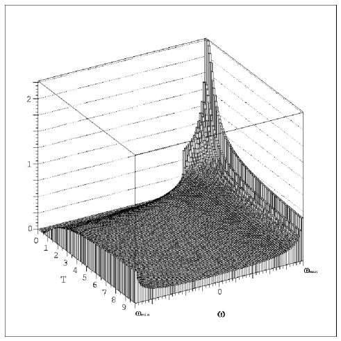
FIG. 5.: Longitudinal dynamic structure factor $S^{z}(\pi/2,\omega,T)$ of the $XX$ chain. (See Eq. (10).) Note the sharp cutoff at the lower spectral boundary near $T=0$.

FIG. 6.: Transversal dynamic structure factor $S^{x}(q=\pi/2,\omega,T)$. The $T=const$ cross section becomes an exact Gaussian for $T=\infty$.

FIG. 7.: Temperature dependence of the longitudinal dynamic structure factor $S^{z}(3\pi/4,\omega)$ of the $N=16$ $XXZ$ chain with $\Delta=\cos(0.3\pi)$. $T$ varies from $0.2J$ (front) to $19.7J$ (back). The two-spinon continuum ranges from $\omega=1.907J$ to $\omega=4.983J$. Note that the $x$ axis represents $-\omega/J$ for reasons of visibility.

FIG. 8.: Same as Fig.7, for the transverse dynamic structure factor $S^{x}(3\pi/4,\omega)$. The boundaries of the excitation continua are $\varepsilon_{1}=1.907J,\varepsilon_{2}=4.983J,$ and $\tilde{\varepsilon}_{2}=2.064J$. The $x$ axis represents $-\omega/J$ for reasons of visibility.

FIG. 9.: Temperature dependence of the dynamic structure factor $S^{z}(3\pi/4,\omega)$ of the $N=16$ isotropic Heisenberg chain. $T$ varies from $0.2J$ (front) to $19.7J$ (back). The two-spinon continuum ranges from $2.22J$ to $5.803J$. The $x$ axis represents $-\omega/J$ for reasons of visibility.

FIG. 10.: Dynamic structure factor $S^{z}(7\pi/8,\omega)$ of the $XXX$-chain at $T=1.2J$. Shown are the numerical result from a $N=16$ chain (solid line) and the field-theoretical result of Schulz, Eq. (23) (dashed line).

FIG. 11.: Same as Fig.10, for $T=2.7J$.

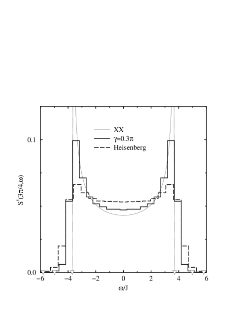
FIG. 12.: Longitudinal dynamic structure factor $S^{z}(3\pi/4,\omega)$ of the $N=16$ $XXZ$ chain at $T=\infty$, for $\Delta=1$ (dashed line) and $\Delta=\cos(0.3\pi)$ (solid line). For comparison we also show the exact $N=\infty$ result for the $XX$ chain, $\Delta=0$ (thin line). The three pairs of triangles on the frequency axis mark the upper boundary $\pm\varepsilon_{2}(\frac{3\pi}{4})$ (20) of the two-spinon continuum for $\Delta=0,\cos(0.3\pi)$, and 1 (in ascending order of $|\omega|$).

FIG. 13.: Transversal dynamic structure factor: logarithm of $S^{x}(q,\omega)$ of the $N=16$ $XXZ$-chain with $\gamma=0.3\pi$ and $\gamma=0.5\pi$ at $T=\infty$. a: $q=\frac{\pi}{2}$ for $\gamma=0.3\pi$ and the q-independent Gaussian for $\gamma=0.5\pi$. b: $\gamma=0.3\pi$ and $q=0,\pi/2$ and $\pi$.

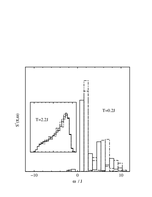
FIG. 14.: Finite-size effects in $S^{z}(\pi,\omega)$ for $\gamma=0.3\pi$ at $T=0.2J$ (main plot) and $T=2.2J$ (inset). Data for $N=12,14,$ and 16 are shown as dot-dashed, dashed, and solid lines, respectively.

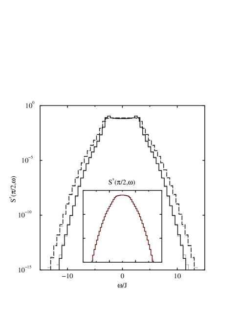
FIG. 15.: Absence of finite-size effects at $T=\infty$ in the low-weight spectral tails. Main plot: $S^{z}(\pi/2,\omega)$ at $\gamma=0.3\pi$ (solid line) and $\gamma=0$ (dashed line). Inset: $S^{x}(\pi/2,\omega)$ at $\gamma=0.3\pi$(same range of variables as main plot). Data for $N=12$ are shown as thin lines, those for $N=16$ as heavy lines.

FIG. 16.: Real part of the $z$ spin pair correlation function $\langle S_{l}^{z}(t)S_{l+n}^{z}\rangle$ for $n=0$ (top) through 8 (bottom), at $T/J=20$, for anisotropy $\Delta=\cos(0.3\pi)$ and different system sizes, $N\geq 2n$, namely $N=16$ (solid lines), $N=14$ (dashed), and $N=12$ (dot-dashed). (Curves are displaced in the vertical direction for graphical purposes.)

FIG. 17.: The intermediate structure factor $I^{z}(q=\pi,t,T=\infty)$ for the $XXX$-chains of 14 and 16 spins and the upper and lower boundaries (dashed lines) from Ref.[25]. The curves for $N=14$ and $N=16$ can not be distinguished on this scale.

FIG. 18.: Real part (upper set of curves) and imaginary part (lower set of curves) of the $z$ spin autocorrelation function $\langle S_{l}^{z}(t)S_{l}^{z}\rangle$ for temperatures $T/J=20,2,0.7,$ and $0.2$ (top to bottom in each set of curves), for anisotropy $\Delta=\cos(0.3\pi)$ and different system sizes, $N=16$ (solid lines), $N=14$ (dashed), and $N=12$ (dot-dashed). (Curves are displaced in the vertical direction for graphical purposes; the $y$-axis scale applies to the uppermost curve; Re$\langle S_{l}^{z}(0)S_{l}^{z}\rangle=1$, Im$\langle S_{l}^{z}(0)S_{l}^{z}\rangle=0$ for arbitrary $T$.)

FIG. 19.: Real part of the $x$ spin autocorrelation function $\langle S_{l}^{x}(t)S_{l}^{x}\rangle$ of the $XX$ chain $(\Delta=0)$ for temperatures $T/J=2$, $20$, and $\infty$, and system sizes $N=16$ (solid lines) and $N=14$ (dashed lines; no $N=14$ data shown for $T=\infty$). The $N=16$ result for $T=\infty$ coincides with the exact result for $N=\infty$ following by Fourier transformation from (13). The inset shows the $N=16$ results for $T=\infty$, $\Delta=0$ (dot-dashed), $\Delta=\cos(0.3\pi)$ (solid line), and $\Delta=1$ (dashed line).

FIG. 20.: Real part of the $z$ spin autocorrelation function $\langle S_{l}^{z}(t)S_{l}^{z}\rangle$ of the $XXZ$ chain for $N=16$ and temperatures $T/J=\infty$ (main plot) and $0.2$ (inset).

FIG. 21.: The intermediate structure factor at $T=\infty$. The solid curve represents $|I^{z}(q=\pi,t,\Delta=\cos(0.3\pi))|$, the dotted $|I(q=\pi,t,\Delta=1)|$ and the dashed $|I^{x}(q=\pi,t,\Delta=\cos(0.3\pi)|$. For reasons of visibility the upper (lower) curve is multiplied by a factor of 10 (0.1). The straight lines are drawn through the fourth and fifth maxima.

REFERENCES

- [1] E. Balcar, S.W. Lovesey, Theory of magnetic neutron and photon scattering, Oxford (Clarendon Press) 1989.
- [2] E. Lieb, T. Schultz, and D. Mattis, Ann. Phys. (N.Y.) 16, 407 (1961).
- [3] S. Katsura, Phys. Rev. 127, 1508 (1962).
- [4] Th. Niemeijer, Physica 36, 377 (1967).
- [5] S. Katsura, T. Horiguchi, and M. Suzuki, Physica 46, 67 (1970).
- [6] B. M. McCoy, E. Barouch, and D.B. Abraham, Phys. Rev. A 4 2331 (1971).
- [7] H. G. Vaidya and C. A. Tracy, Physica 92A, 1 (1978).
- [8] B. M. McCoy, J. H. H. Perk, and R. E. Shrock, Nucl. Phys. B 220, [FS8], 35 (1983), 269 (1983).
- [9] G. Müller and R. E. Shrock, Phys. Rev. B 29, 288 (1984).
- [10] A. Sur, D. Jasnow, and I.J. Lowe, Phys. Rev. B 12, 3845 (1975).
- [11] U. Brandt and K. Jacoby, Z. Physik B 25, 181 (1976).
- [12] H.W. Capel and J.H.H. Perk, Physica 87A, 211 (1977).
- [13] A. R. Its, A. G. Izergin, V. E. Korepin, and N. A. Slavnov, Phys. Rev. Lett. 70, 1704 (1993).
- [14] I.S. Gradshteyn and I.M. Ryzhik, Table of Integrals, Series, and Products, New York (Academic Press) 1980 (formula 8.531.3).
- [15] A. Luther and I. Peschel, Phys. Rev. B 12, 3908 (1975).
- [16] H. C. Fogedby, J. Phys. C 11, 4767 (1978).
- [17] At first sight there seems to be a contradiction between for and the universal behavior of for the case discussed earlier. However, it must be kept in mind that the continuum field theory of Refs.[15] and [16] is unable to account for lattice effects such as the existence of a high-frequency cutoff in the particle-hole spectrum of noninteracting fermions which causes the contribution for the case.
- [18] K. Fabricius, U. Löw and K.-H. Mütter, J. Phys.: Condens. Matter 7, 5629 (1995).
- [19] G. Müller, H. Thomas, M. Puga, and H. Beck, J. Phys. C (Cond. Mat.) 14, 3399 (1981).
- [20] A.H. Bougourzi, M. Couture, and M. Kacir, Stony Brook preprint ITP-SB-96-21 (q-alg 9604019).
- [21] M. Karbach, G. Müller, and A.H. Bougourzi, University of Rhode Island preprint (cond-mat 9606068).
- [22] H.J. Schulz, Phys. Rev. B 34, 6372 (1986).
- [23] D.A. Tennant, R.A. Cowley, S.E. Nagler, and A.M. Tsvelik, Phys. Rev. B 52, 13368 (1995).
- [24] M. Steiner, J. Villain, C.G. Windsor, Advances in Physics, 25, 87 (1976).
- [25] M. Böhm and H. Leschke, J. Phys. A 25, 1043 (1992).
- [26] A. Sur and I.J. Lowe, Phys. Rev. B 11, 1980 (1975).
- [27] J.M.R. Roldan, B.M. McCoy, and J.H.H. Perk, Physica A 136, 255 (1986).
- [28] B.M. McCoy, in “Statistical Mechanics and Field Theory”, (World Scientific 1995), eds. V.V. Bazhanov and C.J. Burden.
- [29] X. Zotos, P. Prelovšek, Phys. Rev. B 53, 983 (1996).
- [30] B.N. Narozhny, Phys. Rev. B 54, 3311 (1996).
- [31] M. Böhm, V.S. Viswanath, J. Stolze, and G. Müller, Phys. Rev. B 49, 15669 (1994).
- [32] M. Böhm, H. Leschke, M. Henneke, V.S. Viswanath, J. Stolze, and G. Müller, Phys. Rev. B 49, 417 (1994).
- [33] H. Bethe, Z. Phys. 71, 205 (1931).
- [34] J. des Cloizeaux and J.J. Pearson, Phys. Rev. 128, 2131 (1962).
- [35] T. Yamada, Prog. Theor.Phys. 41, 880 (1969).
- [36] G. Müller, H. Thomas, H. Beck, and J.Bonner, Phys. Rev. B 24, 1429 (1981).
- [37] L.D. Faddeev and L.A. Takhtajan, Phys. Lett. 85A, 375 (1981).
- [38] L.D. Faddeev and L.A. Takhtajan, J. Sov. Math. 24, 241 (1984).
- [39] F. Woynarovich, J. Phys. A: Math. Gen. 15, 2985 (1982).
- [40] F.D.M. Haldane and M.R. Zirnbauer, Phys. Rev. Lett. 71, 4055 (1993).
- [41] J.C. Talstra and F.D.M. Haldane, Phys. Rev. B 50, 6889 (1994).
- [42] F.D.M. Haldane, Phys. Rev. Lett. 60, 635 (1988).
- [43] F.D.M. Haldane, Phys. Rev. Lett. 66, 1529(1991).
- [44] B.S. Shastry, Phys. Rev. Lett 60, 639 (1988).
- [45] J.C. Talstra, Thesis, Princeton 1995 (cond-mat 9509178).
- [46] G.Castilla, S.Chakravarty, and V.J.Emery, Phys. Rev. Lett 75 1823 (1995).
- [47] M.Matsuda, and K.Katsumata , Phys. Rev. B 53, 12201 (1996).
- [48] J. Stolze, A. Nöppert, and G. Müller, Phys. Rev. B 52, 4319 (1995).
- [49] The constant in (23) was fixed so that satisfactory agreement to the numerical data was obtained for all and both and .
- [50] The relative deviation between the and results is less than for ; it grows to about for .
- [51] Colleagues who wish to obtain some of our numerical data for comparison with their own work are invited to send an e-mail to Klaus.Fabricius@wptu13.physik.uni-wuppertal.de .
- [52] It should be remarked that for , the N=14 curves coincide with N=16, so in the time range we can be sure that our results represent the thermodynamic limit.
- [53] R. B. Griffiths, Phys. Rev. 133, A768 (1964).