Fractional vortices on grain boundaries — the case for broken time reversal symmetry in high temperature superconductors

Abstract

We discuss the problem of broken time reversal symmetry near grain boundaries in a $d$-wave superconductor based on a Ginzburg-Landau theory. It is shown that such a state can lead to fractional vortices on the grain boundary. Both analytical and numerical results show the structure of this type of state.

]

I Introduction

During the last few years the understanding of the microscopic properties of the high-temperature superconductors (HTSC) has gradually improved [1]. While for a long time studies have focused on the exotic normal state properties, recently the interest turned more towards the superconducting phase, in particular, the symmetry of the order parameter. For a tetragonal system the list of possible order parameter symmetries is rather long [2]. However, the recent debate has essentially concentrated only on two symmetries of the Cooper pair wavefunction [3]. One is due to “$s$-wave” pairing, the most symmetric pairing channel. The other is “$d$-wave” pairing, where the pair wavefunction ($\psi({\bf k})\propto\cos k_{x}-\cos k_{y}$) changes sign under $90^{o}$-rotations in the basal plane of the tetragonal crystal lattice. As a consequence, the latter wave function has nodes along the [110]-direction. A possible alternative to the standard $s$-wave was presented with the “extended $s$-wave” pairing state ($\psi({\bf k})\propto\cos k_{x}+\cos k_{y}$) which has also nodes in the first Brillouin zone, but is completely symmetric under all operations of the tetragonal point group $D_{4h}$ [4]. For the orthorhombically distorted system, the $s$- and $d$-wave channels are not distinguished by symmetry. Nevertheless, we expect that basic properties of the pair wave function such as the existence of sign changes and nodes are retained if they were present in the tetragonal case [5].

A variety of experiments have been performed in order to distinguish among the order parameter symmetries. One class of experiments considers the properties of the quasi particle excitations in the superconducting state. The existence of nodes in the pair wavefunction implies that there are also nodes in the excitation gap. Low-lying excitations at the nodes modify the low-temperature behavior of certain thermodynamic properties compared with that of a superconductor which opens a complete gap. The clearest sign of such an effect was observed for the London penetration depth which behaves as $\lambda(T)-\lambda(0)\propto T$ in contrast to the conventional exponential law, $\propto\exp(-\Delta/k_{B}T)$ [6]. This result strongly suggests that there are nodes in the gap and the pair wavefunctions, which are compatible with both extended $s$-wave and $d$-wave as well as with a very anisotropic $s$-wave state.

Another class of experiments aims at the direct observation of the intrinsic phase structure, the sign changes of the pair wavefunction. The Josephson effect as a phase coherent coupling of the order parameters of two superconductors provides the natural means for this purpose [8, 9]. Arrangements connecting YBCO single crystals at two perpendicular surfaces to a standard $s$-wave superconductor to form a loop for a SQUID have been used to detect a phase difference between the $x$- and $y$-direction of the pair wavefunction [10]. The experiments observe with good precision a phase difference of $\pi$ compatible with the $d_{x^{2}-y^{2}}$-wave order parameter.

The intrinsic $\pi$ phase shift in this configuration leads to frustration effects which manifest themselves in the form of a spontaneous supercurrent flowing around the loop. The supercurrent generates a flux $\Phi=\pm\Phi_{0}/2$ where $\Phi_{0}=hc/2e$ is the standard flux quantum. This property has recently been detected and the flux was measured with very high accuracy [11].

On the other hand, several other experiments based on the Josephson effect seem at present to contradict the presence of a $d$-wave order parameter. Chaudhari and Lin analyzed the Josephson current through a grain boundary in the basal plane with a special geometry giving a basal plane contact between two segments of a YBCO film [12]. They demonstrated that various properties might support an order parameter with $s$-wave rather than simple $d$-wave symmetry. The interpretation of this experiment, however, has recently been contested by Millis [13]. In contrast, Sun and coworkers investigated Josephson tunneling between a standard $s$-wave superconductor (Pb) and YBCO, where the tunneling direction is the $c$-axis of YBCO [14]. These data so far could not be explained consistently within the picture of pure $d$-wave superconductivity. Therefore, the simple $d$-wave scenario may not be sufficient for a complete understanding of all experiments introduced here [15].

Indeed a recent experiment by Kirtley and coworkers suggests that the situation is more complicated than might be naively expected for a $d$-wave superconductor [16]. Their experimental arrangement consists of two segments of $c$-axis textured YBCO films where one is a triangular inclusion within in the other. The basal plane crystalline axes are misaligned with one another. The boundary of the triangle acts as junction between the two segments. We will show in Section II that if YBCO were a $d$-wave superconductor we would expect vortices to appear spontaneously at two of the three corners of the triangle each containing a flux of $\pm\Phi_{0}/2$. The experiment does find spontaneous vortices at corners, but these vortices have fluxes different from $n\Phi_{0}/2$ ($n$: integer). In addition, flux appears at all three corners and occasionally also on an edge of the triangle. We will argue in Section II that this can be explained by a superconducting state which violates time-reversal symmetry ${\cal T}$. Therefore, the simple picture of a single component $d_{x^{2}-y^{2}}$-wave order parameter might not apply here.

${\cal T}$-violation is not uncommon in the field of unconventional superconductivity. A large number of superconducting states classified by symmetry indeed break time-reversal symmetry [2, 17]. In the complex superconducting phase diagrams of the heavy fermion compounds, ${\rm UPt}_{3}$ and $U_{1-x}{\rm Th}_{x}{\rm Be}_{13}$ ($0.02\leq x\leq 0.045$) states appear which probably break time-reversal symmetry. It was shown theoretically that such superconducting states can generate spontaneous supercurrents and magnetic field distributions in the vicinity of lattice defects and surfaces [18]. In both compounds the occurrence of such local fields in connection with the superconducting phase transition has been detected by means of muon spin rotation ($\mu$SR) measurements [19]. For both compounds, consistent phenomenological theories for this effect have been formulated [17].

In the field of HTSC, various theories and mechanisms leading to ${\cal T}$-violating superconducting states have been proposed. The effective two-dimensionality of the cuprates may serve as a basis for particles with fractional statistics, the so-called anyons [20]. Laughlin showed that the resulting superconducting state has a composite order parameter of the form $d_{x^{2}-y^{2}}+i\epsilon d_{xy}$ which obviously breaks time-reversal symmetry [21]. Alternative mechanisms can lead to a ${\cal T}$-violating states with the symmetry $s+id_{x^{2}-y^{2}}$ [22]. At present there is no indication beyond any doubt that such states are realized in the HTSC [23]. On the contrary, recent experiments demonstrate that at least at the onset of superconductivity ($T\approx T_{c}$) the critical behavior of the London penetration depth is that of a single component order parameter belonging to the universality class of the XY-spin model [24]. Only below an additional superconducting transition at lower temperature could the composite ${\cal T}$-violating order parameter appear. No signs of such an additional phase transition have yet been observed in the thermodynamic properties. In addition, it should be noted that each of the ${\cal T}$- violating states mentioned above lacks gap nodes. This fact would also lead to inconsistency with low-temperature measurements of the London penetration depth which demonstrate the presence of nodes, as mentioned above [6].

In this paper we will show that there is no conflict between the interpretation of the experiment by Kirtley and coworkers [16] which could indicate ${\cal T}$-violation and the other experiments which obviously rule out the existence of such a state [25]. We argue that the latter experiments address bulk properties, while the former one considers effects in connection with interfaces and grain boundaries. The seeming conflict is resolved when we assume that ${\cal T}$-violation occurs only locally in the immediate vicinity of an interface. The bulk, on the other hand, may only have a single component order parameter, presumably with $d$-wave symmetry, but we cannot rule out other symmetries. As we will discuss below, the extension of the ${\cal T}$-violating state towards the bulk is rather short, of the order of coherence length $\xi$.

II A first interpretation of the experiment

Let us now examine the properties of an arrangement similar to the one used by Kirtley and coworkers [16]. As illustrated in Fig. 1a, it is a superconducting film of triangular shape as an inclusion in another superconducting film, both of the same material. The crystal symmetry is tetragonal (for simplicity we neglect here the orthorhombic distortion present in many HTSC) and the film is $c$-axis textured. The basal plane axes (of the inclusion and the surrounding) are misoriented with each other. The interfaces (the edges of the triangle, each of length $L$) are weak links between the inner and the outer film. For simplicity we will treat them as Josephson contacts so that the standard sinusoidal current-phase relation applies.

A Pure $d$-wave symmetry

Let us analyze the properties of this arrangement under the assumption that the superconductor here is a $d$-wave superconductor with an order parameter symmetry as the pair wavefunction $\psi_{d}({\bf k})=\cos k_{x}-\cos k_{y}$. This means that we should carefully consider the intrinsic phase structure of the order parameter when deriving the Josephson current-phase relation. The phase difference between the positive and negative lobes of the pair wavefunction is $\pi$. If dominant lobes of the same sign face each other at an interface, the corresponding Josephson current-phase relation has the standard form and the interface energy is minimized by a vanishing difference the order parameter phases (0-junction). However, if the facing lobes have opposite sign, an additional phase $\pi$ enters and the energy is minimized by a phase difference of $\pi$ ($\pi$-junction) [9]. We have

$$E_{J}(\varphi)=-\frac{I_{c}\Phi_{0}}{2\pi c}\cos(\varphi-\alpha)$$ (1)

where $\alpha=0$ for a 0-junction and $\pi$ for a $\pi$-junction, and $\varphi$ is the phase difference through the interface. In Fig. 1a we assume that the edge segments 1-2 and 3-1 can be labeled as a $\pi$-junction and segment 2-3 as a 0-junction. This definition is not unique. A redefinition of the order parameter phase in one of the two superconductors ($\phi\to\phi+\pi$) would reverse this labeling.

FIG. 1.: Triangular grain boundary in a $d$-wave superconductor: (a) The edges act as Josephson junctions with phase shifts, 0 or $\pi$; (b) The phase $\varphi$ tries to be pinned at phase shift values (indicated by dashed lines) and change in an antikink (kink) of width $\lambda_{J}$ at the corners 2 and 3. There are several possible solutions for $\varphi$ due to the $2\pi$-periodicity of the phase. The solution with an anti-kink and a kink leads to an overall phase winding 0 around the triangle. An equivalent solution with two kinks (also shown) would give $2\pi$ winding.

We now map all segments of the interface onto a one-dimensional axis with periodic boundary conditions for the coordinate $\tilde{x}$ as shown in Fig. 1b ($\tilde{x}+3L=\tilde{x}$). Here we can study the spatial variation of $\varphi$ along $\tilde{x}$ by using the Sine-Gordon equation

$$\partial_{\tilde{x}}^{2}\varphi=\lambda^{-2}_{J}\sin(\varphi-\alpha(\tilde{x})),$$ (2)

where both the Josephson penetration depth $\lambda_{J}=(\phi_{0}c/8\pi^{2}dI_{c})^{1/2}$ ($d$: magnetic width of the interface) and the intrinsic phase shift $\alpha$ are assumed to be constant within each segment (see Fig.1b) [26]. For good junctions ($\lambda_{J}\ll L$), $\varphi$ tends to be pinned to the value $\alpha$ in each segment of the interface, but has to change at the boundaries where $\alpha$ is discontinuous. The solution of Eq.(2) shows kinks at these boundaries with an extension of $\lambda_{J}$ (Fig. 1b). Note that the two kinks at 2 and 3 can be either “kink” and “anti-kink” or both “kinks” as a consequence of the periodicity of Eq. (2). Other types of kink solutions are energetically more expensive.

The spatial variation of $\varphi$ induces a local magnetic flux density on the interface given by the expression $\phi(\tilde{x})=\Phi_{0}\partial_{\tilde{x}}\varphi(\tilde{x})/2\pi$ Therefore, each kink corresponds to a local flux line or vortex with a magnetic flux $\Phi=\Phi_{0}(\varphi_{r}-\varphi_{l})/2\pi$, where $\varphi_{r(l)}$ denotes the values of $\varphi$ far enough to the right (left) of the kink such that $\partial_{\tilde{x}}\varphi$ is essentially zero. Both kinks in Fig. 1b indicate vortices with $\Phi=\pm\Phi_{0}/2$. Due to the periodicity of $\tilde{x}$ we find that $\varphi(\tilde{x}+3L)=\varphi(\tilde{x})+2\pi n$ ($n$: integer), which requires that the total flux integrated over the whole triangle interface be an integer multiple of $\Phi_{0}$. Of course, the triangle is surrounded by a superconductor whose single valued order parameter allows phase windings of $2\pi n$ only. This “sum rule” implies that half-integer flux lines can only appear at two of the three corners. Because the flux on each corner can only vary by $n\Phi_{0}$, at corner 2 and 3 there is always a flux line with a flux of at least $\Phi_{0}/2$. Larger fluxes could be stabilized by an external field. This result is equivalent to the one presented in Ref. 8 and 13.

The comparison of our “experiment” with the one performed in reality shows that the simple picture we tried to draw here does not explain the measurement by Kirtley and coworkers [16]. They found fluxes at all corners, all of which are clearly smaller than $\Phi_{0}/2$. We call them fractional vortices. In all samples checked, the sum rule constraining the total flux on the boundary to an integer multiple of $\Phi_{0}$ was satisfied with good accuracy.

In the introduction we claimed that the existence of fractional vortices requires a superconducting phase with broken time-reversal symmetry. We give here a brief argument for this statement. Consider one of the corners of the triangle (or a similar structure) with a vortex whose flux is $\Phi$. Apply the time-reversal operation to this system. This reverses the flux ($\Phi\to-\Phi$). If the superconductor is otherwise invariant under this operation (${\cal T}$-invariant), the difference between $\Phi$ and $-\Phi$ must be an integer multiple of $\Phi_{0}$ as in every standard superconductor: $\Phi=-\Phi+n\Phi_{0}$. Therefore, $\Phi$ ($=n\Phi_{0}/2$) is an integer or half-integer quantum of $\Phi_{0}$ as seen above. Consequently the observation of a vortex with a flux different from those values can only mean that the superconducting state is not invariant under the time-reversal operation [27].

B Josephson effect for a ${\cal T}$-violating interface

A ${\cal T}$-violating superconducting order parameter consists of at least two components (e.g., $d_{x^{2}-y^{2}}+id_{xy}$ or $s+id_{x^{2}-y^{2}}$). We therefore restrict ourselves to the case of a two-component order parameter with a generic pair wave function $\psi({\bf k})=\eta_{1}\psi_{1}({\bf k})+\eta_{2}\psi_{2}({\bf k})$. Here $\eta_{1}$ and $\eta_{2}$ are the two complex order parameters with the symmetry properties of the corresponding pair wavefunctions. Time-reversal transforms the order parameter to its complex conjugate ($\eta_{j}\to\eta^{*}_{j}$). If time-reversal symmetry is conserved, then $(\eta_{1},\eta_{2})$ is up to a common phase factor equal to $(\eta^{*}_{1},\eta^{*}_{2})$ or $\eta_{1}/\eta_{2}=\eta^{*}_{1}/\eta^{*}_{2}$. Otherwise, the order parameter breaks time-reversal symmetry and the state is at least two-fold degenerate, since both $(\eta_{1},\eta_{2})$ and $(\eta^{*}_{1},\eta^{*}_{2})$ have the same free energy. We will consider here the standard situation where $\eta_{1}/\eta_{2}$ is imaginary: $\phi_{1}-\phi_{2}=\pm\pi/2$ ($\eta_{j}=|\eta_{j}|\exp(i\phi_{j})$).

For an interface between two superconductors ($A$ and $B$) both with order parameter $(\eta^{A(B)}_{1},\eta^{A(B)}_{2})$ the Josephson current phase relation has the form

$$J=\sum^{2}_{i,j=1}J_{cij}\sin(\phi^{B}_{i}-\phi^{A}_{j})$$ (3)

where $J$ is the supercurrent density at a given point on the interface. There are four different combinations for the phase coherent coupling and $J_{cij}$ denotes the coupling strength between the components $\eta^{B}_{i}$ on side $B$ and with $\eta^{A}_{j}$ on side $A$ ($\eta^{\mu}_{j}=|\eta^{\mu}_{j}|\exp(i\phi^{\mu}_{j})$) with $j=1,2$ and $\mu=A,B$). The energy for a uniform interface of area $S$ is given by

$$E_{J}=-\frac{\Phi_{0}S}{2\pi c}\sum^{2}_{i,j=1}J_{cij}\cos(\phi^{B}_{i}-\phi^{A}_{j})$$ (4)

For simplicity we restrict ourselves to the situation where $\phi^{A}_{1}-\phi^{A}_{2}=\phi^{B}_{1}-\phi^{B}_{2}=\pi/2$ is fixed on both sides of the interface. (This phase difference can be different in the vicinity of the junction without changing the conclusion we will draw here for the simplified case.) The current density $J$ and the interface energy density $\epsilon_{J}$ depend only on one phase difference through the interface, say $\varphi=\phi^{B}_{1}-\phi^{A}_{1}$.

$$\begin{array}[]{l}\displaystyle J(\varphi)=\tilde{J}_{c}\sin(\varphi-\tilde{\alpha})\\ \\ \displaystyle\epsilon_{J}(\varphi)=-\frac{\Phi_{0}\tilde{J}_{c}S}{2\pi c}\cos(\varphi-\tilde{\alpha})\\ \end{array}$$ (5)

with

$$\begin{array}[]{l}\displaystyle\tilde{J}_{c}=\sqrt{(J_{c11}+J_{c22})^{2}+(J_{c12}-J_{c21})^{2}}\\ \\ \displaystyle\tan(\tilde{\alpha})=\frac{J_{c12}-J_{c21}}{J_{c11}+J_{c22}}\\ \end{array}$$ (6)

The phase shift $\tilde{\alpha}$ corresponds to $\varphi$ minimizing the interface energy. In this sense the correct solution for $\tilde{\alpha}$ must be chosen in Eq. (6) [8]. Obviously, $\tilde{\alpha}$ can assume any value and depends only on the relative magnitude of the different coupling components which parameterize here the interface properties. It is easy to follow the same consideration for the ${\cal T}$-invariant combination of $\eta_{1}$ and $\eta_{2}$ where we find that $\tilde{\alpha}$ is strictly either 0 or $\pi$.

Let us apply this result to the triangle studied above, assuming ${\cal T}$-violating superconducting states. Each of the interface segments as a uniform junction is characterized by a phase shift $\tilde{\alpha}$ ($0<\tilde{\alpha}<\pi$). Analyzing Eq. (2) for this situation we find that there are now kinks of $\varphi$ at all three corners connecting the different values of $\tilde{\alpha}$ in each segment (Fig.2). This leads to vortices at these corners whose fluxes are given by

$$\Phi=\Phi_{0}\frac{\tilde{\alpha}_{r}-\tilde{\alpha}_{l}}{2\pi}$$ (7)

with $\tilde{\alpha}_{r(l)}$ as the values of $\tilde{\alpha}$ on the segments on right (left) of the corner. It is obvious that in this case the flux $\Phi$ need not be $\Phi_{0}$ or $\Phi_{0}/2$. Thus, these kinks correspond to what we described as fractional vortices above. Note, that also here the sum of all fluxes must add up to an integer multiple of $\Phi_{0}$ because of the periodic boundary condtions for $\varphi$.

FIG. 2.: Phase $\varphi$ for a triangle with ${\cal T}$-violating interface states. The phase shifts $\alpha_{ij}$ are indicated by the dashed line. $\varphi$ follows these phase shifts by creating (anti-)kinks at all three corners. The kink heights are different from a multiple of $\pi$ in general and lead to fractional fluxes.

III The interface state

As mentioned earlier, the assumption of a ${\cal T}$-violating bulk superconducting state is incompatible with a number of experiments. It is, however, possible that ${\cal T}$-violation occurs only in the vicinity of the interface (grain boundary). This is enough to generate fractional vortices at grain boundary corners. In this section we would like to discuss such an interface state based on a Ginzburg-Landau theory.

A Ginzburg-Landau theory

We use a Ginzburg-Landau free energy functional of two complex order parameters $\eta_{1}$ and $\eta_{2}$. The first order parameter shall be the dominant one corresponding to the $d_{x^{2}-y^{2}}$-wave pairing state. For the second we choose the $d_{xy}$-wave pairing state. Thus the pairing state is a combination of the two components

$$\psi({\bf k})=\sum_{i=1,2}\eta_{i}\psi_{i}({\bf k})=\eta_{1}\psi_{1}({\bf k})+\eta_{2}\psi_{2}({\bf k})$$ (8)

with

$$\psi_{1}({\bf k})=k^{2}_{x}-k^{2}_{y}\qquad\mbox{and}\qquad\psi_{2}({\bf k})=k_{x}k_{y}.$$ (9)

The free energy functional must be invariant under the symmetry transformations of the crystal group (in this case tetragonal,$D_{4h}$), time reversal and U(1)-gauge symmetry. Keeping terms up to fourth order in the expansion with respect to order parameter, we have

$${\cal F}=\int d^{2}x\,[{\cal F}_{I}+{\cal F}_{12}+{\textstyle\sum_{i=1,2}}{\cal F}_{i}]$$ (10)

where

$${\cal F}_{i}=\alpha_{i}|\eta_{i}|^{2}+\frac{\beta_{i}}{2}|\eta_{i}|^{4}+K_{i}|{\bf D}\eta_{i}|^{2}$$ (11)

$${\cal F}_{12} = \gamma|\eta_{1}|^{2}|\eta_{2}|^{2}+\delta(\eta_{1}^{2}\eta_{2}^{*2}+\,\mbox{c.c.})+\kappa^{2}(\nabla\times{\bf A})^{2}$$ (12)

$$+ \tilde{K}\left((D_{x}\eta_{1})^{*}(D_{y}\eta_{2})-(D_{y}\eta_{1})^{*}(D_{x}\eta_{2})+\,\mbox{c.c.}\right)$$ (13)

$${\cal F}_{I} = \sum_{i=1,2}\{g_{i}^{A,B}|\eta_{i}^{A,B}|^{2}$$ (14)

$$- \frac{\Phi_{0}}{2\pi c}\sum_{j=1,2}\tilde{J}_{ij}{\rm Re}\,\eta_{i}^{B}\eta_{j}^{*A}\}\delta({\sl interface}).$$ (15)

We work in units where ${\bf D}=\nabla-i2\pi{\bf A}/\Phi_{0}$ (${\bf A}$: vector potential). The coefficients are all phenomenological parameters which contain the relevant information of microscopic origin. The second order coefficients depend on the temperature in the usual way ($\alpha_{i}=a^{\prime}(T-T_{ci})$ where $T_{ci}$ is the bare transition temperature of $\eta_{i}$). The interface free energy ${\cal F}_{I}$ includes the pair breaking effect in the first term and the Josephson junction energy in the second term (note: $\tilde{J}_{12}=\tilde{J}_{21}$). The superscripts $B$ and $A$ denote the different sides of the interface, or “outside” and “inside” if the interface is a closed curve.

It is worth noting that the free energy expansion without interface term is cylindrical symmetric with $z$ as the rotation axis, although the system has only tetragonal symmetry. Anisotropy enters via the interface term. The coefficients $g_{i}$ and $\tilde{J}_{ij}$ depend in general on the angle between crystal axes and the interface. Pair breaking for the $d_{x^{2}-y^{2}}$-wave ($d_{xy}$-wave) phase is most effective when the interface normal vector points along the [1,1] ([1,0])-direction, i.e. along the nodes of the pair wavefunction [17]. On the other hand, pair breaking is weaker when the lobes of the pair wavefunctions point towards the interface. Consequently, the $d_{x^{2}-y^{2}}$-wave component of the order parameter is suppressed weakly where the $d_{xy}$-wave component is affected most (and vice versa). Similarly, the interface coupling coefficients depend on the internal structure of the pair wavefunction. If we denote the angle between the interface normal vector and the crystalline $x$-axis by $\vartheta$, they are $\tilde{J}_{ij}=J_{0}f_{i}(\vartheta_{B})f_{j}(\vartheta_{A})$, where the functions have the generic angular structure $f_{1}(\vartheta)=\cos(2\vartheta)$ and $f_{2}(\vartheta)=\sin(2\vartheta)$ which indicate the internal phase structure of the two pair wavefunctions.

The variation of ${\cal F}$ with respect to $\eta_{i}$ and ${\bf A}$ yield the following Ginzburg-Landau equations:

$$K_{i}{\bf D}^{2}\eta_{i} = \alpha_{i}\eta_{i}+\beta_{i}|\eta_{i}|^{2}\eta_{i}+\gamma|\eta_{3-i}|^{2}\eta_{i}$$ (16)

$$+ 2\delta\eta_{3-i}^{2}\eta_{i}^{*}-(-1)^{i}\tilde{K}B_{z}\eta_{3-i}$$ (17)

and

$$\kappa^{2}\mathchoice{{\hbox{\boldmath$\displaystyle\nabla$}}}{{\hbox{\boldmath$\textstyle\nabla$}}}{{\hbox{\boldmath$\scriptstyle\nabla$}}}{{\hbox{\boldmath$\scriptscriptstyle\nabla$}}}\times(\mathchoice{{\hbox{\boldmath$\displaystyle\nabla$}}}{{\hbox{\boldmath$\textstyle\nabla$}}}{{\hbox{\boldmath$\scriptstyle\nabla$}}}{{\hbox{\boldmath$\scriptscriptstyle\nabla$}}}\times{\bf A})=\kappa^{2}{\bf j} = \sum_{i=1,2}K_{i}({\rm Im}\,\eta_{i}^{*}\nabla\eta_{i}-|\eta_{i}|^{2}{\bf A})$$ (18)

$$+ \tilde{K}\nabla\times(\hat{z}\,{\rm Im}\,\eta_{1}\eta_{2}^{*})$$ (19)

The term ${\cal F}_{I}$ generates the boundary condition at the interface with normal vectors ${\bf n}^{A,B}$,

$$K_{i}{\bf n}^{A}\cdot(\mathchoice{{\hbox{\boldmath$\displaystyle\nabla$}}}{{\hbox{\boldmath$\textstyle\nabla$}}}{{\hbox{\boldmath$\scriptstyle\nabla$}}}{{\hbox{\boldmath$\scriptscriptstyle\nabla$}}}-i\frac{2\pi}{\Phi_{)}}{\bf A})\eta^{A}_{i} = g^{A}_{i}\eta^{A}_{i}-\frac{\Phi_{0}}{2\pi c}\sum_{j=1,2}J_{ij}\eta^{B}_{j}$$ (20)

$$K_{i}{\bf n}^{B}\cdot(\mathchoice{{\hbox{\boldmath$\displaystyle\nabla$}}}{{\hbox{\boldmath$\textstyle\nabla$}}}{{\hbox{\boldmath$\scriptstyle\nabla$}}}{{\hbox{\boldmath$\scriptscriptstyle\nabla$}}}-i\frac{2\pi}{\Phi_{)}}{\bf A})\eta^{B}_{i} = g^{B}_{i}\eta^{B}_{i}-\frac{\Phi_{0}}{2\pi c}\sum_{j=1,2}J_{ij}\eta^{A}_{j}$$ (21)

The imaginary part is related to the expression for the supercurrent $j$ perpendicular to the interface and leads to the Josephson current (Eq. (3)) with

$$J_{cij}=J_{ij}|\eta^{B}_{i}||\eta^{A}_{j}|$$ (22)

where the order parameter values are taken at the interface.

Before discussing the interface problem, we consider the properties of the order parameter in the bulk. We assume that $T_{c1}>T_{c2}$ such that for temperatures immediately below $T_{c1}$ only the component $\eta_{1}$ becomes finite, while $\eta_{2}$ remains zero. The instability condition for the occurrence of $\eta_{2}$ is given by

$$\alpha_{2}(T^{*})+(\gamma-2|\delta|)|\eta_{1}(T^{*})|^{2}=0,$$ (23)

defining the transition temperature $T^{*}<T_{c1}$. This second transition leads to a state where both $\eta_{1}$ and $\eta_{2}$ are finite. The relative phase, $\theta=\phi_{1}-\phi_{2}$, depends on the sign of $\delta$. For $\delta<0$ the combination is real, $\theta=0$ or $\pi$ and for $\delta>0$ $\theta=\pm\pi/2$. The latter state breaks time reversal symmetry. For the following we will assume that $\delta>0$. However, the other parameters shall be chosen so that $T^{*}\leq 0$ in order to avoid the second transition as it is not observed in the experiment. We also require that $\gamma>2\delta$ so that the two order parameter components tend to suppress each other.

B Order parameter

We consider now an infinitely extended interface. In this case the order parameter and the vector potential only depend on the coordinate perpendicular to the interface. With certain simplifications a qualitative discussion is possible as we showed in Ref.[25]. We would like to present here an analytical study and then substantiate the result by a complete numerical treatment.

The basic concept leading to an unconventional interface state is the following. Pair breaking at the interface reduces the $\eta_{1}$-component locally. It recovers, however, over a coherence length $\xi=\sqrt{K_{1}/|\alpha_{1}|}$. It is easy to see from Eq. (18) that a local reduction of $\eta_{1}$ leads to a local enhancement of $T^{*}$ (note: $\gamma>2\delta$). Consequently, the $\eta_{2}$-component can appear at the interface at sufficiently low temperature ($T<T^{\prime}$), but it decays exponentially towards the bulk. The extension of $\eta_{2}$ diverges when $T$ approaches the bulk $T^{*}$. Therefore $\eta_{2}$ does not possess the same length scale as $\eta_{1}$ in general. Because $\delta>0$, the combination of $\eta_{1}$ and $\eta_{2}$ is complex $\theta\neq 0$ or $\pi$.

Let us now consider a simplified analytic solution of the Ginzburg-Landau equations for an interface whose normal vector is parallel to the $x$-axis. We neglect the vector potential and the coupling between the two sides ($\tilde{J}_{ij}=0$). A qualitatively good view of the interface state is obtained in the limit where the length scales $\xi_{i}$ of the order parameters are very different, i.e. for $\xi_{1}\ll\xi_{2}$. At the interface, $\eta_{1}$ behaves approximately like

$$\eta_{1}(x)=\eta_{10}{\rm tanh}\left(\frac{|x|+x_{0}}{\xi_{1}}\right)$$ (24)

as can be found by solving the Ginzburg-Landau equation with $\eta_{2}=0$. The boundary condition at the interface determines $x_{0}$ and $\eta_{10}=\sqrt{|\alpha^{*}|/2\beta_{1}}$ is the bulk value of the order parameter. Fixing $\eta_{1}(x)$ the equation for $\eta_{2}$ becomes

$$K_{2}\partial^{2}_{x}\eta_{2} = (\alpha_{2}+\gamma\eta^{2}_{1}(x))\eta_{2}+2\delta\eta^{2}_{1}(x)\eta^{*}_{2}$$ (25)

$$+ \beta_{2}|\eta_{2}|^{2}\eta_{2}+g_{2}\eta_{2}\delta(x)$$ (26)

Following our assumption about the coherence lengths, we approximate the spatial dependence of $\eta_{1}(x)$ by a $\delta$-function in this equation. It is easy to see that $\eta_{2}$ is purely imaginary, $\eta_{2}=iu(x)$ and satisfies the equation

$$K_{2}\partial^{2}_{x}u=\alpha^{*}u+\beta_{2}u^{3}+(g_{2}-(\gamma-2\delta)\eta^{2}_{10}s\xi_{1})\delta(x)$$ (27)

The factor $s$ is of the order one. The solution is a hyperbolic function,

$$u(x)=\sqrt{\frac{2\alpha^{*}}{\beta_{2}}}\frac{1}{{\rm sinh}((|x|+\tilde{x}_{0})/\xi_{2})}$$ (28)

where $\xi^{2}_{2}=K_{2}/\alpha^{*}$. We use the boundary condition at the interface to find the shift $\tilde{x}_{0}$ ($>0$),

$${\rm coth}\left(\frac{\tilde{x}_{0}}{\xi_{2}}\right)=\frac{(\gamma-2\delta)\eta^{2}_{10}\xi^{2}_{2}s-g_{2}\xi_{2}}{2K_{2}}.$$ (29)

Setting the right hand side equal one determines the critical temperature $T^{\prime}$ for the occurrence of $\eta_{2}$. At this point $\tilde{x}_{0}=\infty$. Note that $T^{\prime}>T^{*}$ and that $\eta_{2}$ extends into the whole superconductor when we approach $T=T^{*}$. In the range $T^{*}<T<T^{\prime}$ it decays exponentially on the length $\xi_{2}$. Our numerical results below will show that this approximate solution describes the interface state well apart from the fact that we do not resolve here variations on length scales of $\xi_{1}$.

For finite $\tilde{J}_{ij}$ we can determine the phase shift $\alpha$. In this symmetric formulation of the interface problem the phase shift $\alpha$ would be strictly 0 or $\pi$ even if the state is a complex combination of $\eta_{1}$ and $\eta_{2}$, i.e. it breaks time reversal symmetry. We find immediately that Eqs. (6) and (17) lead to $\alpha=0$ or $\pi$, because $\tilde{J}_{12}=\tilde{J}_{21}$. A condition sufficient for $\alpha$ different from these trivial values would be different coefficients $g_{i}$ on both sides of the interface, which means for example that the crystal orientation on side A and B is different (as it is for a grain boundary). It can be shown that the violation of “parity”, the mirror symmetry due to reflection at the interface, is necessary (see [27]).

C Magnetic properties

The interface state is an inhomogeneous ${\cal T}$-violating superconducting state for temperatures below $T^{\prime}$. It shows unusual magnetic features which originate from an orbital magnetic degree of freedom of the Cooper pairs. Remember that the two pairing components we consider both belong to the $d$-wave channel. If they are combined with a relative phase different from $\theta=0,\pi$, then the pairing state has a component belonging to the spherical harmonic $Y_{2,\pm 2}({\hat{\bf k}})\propto(k_{x}\pm ik_{y})$. This Cooper pair state has a finite orbital magnetic moment $M\hat{{\bf z}}$ parallel to the $z$-axis. The moment generates circular currents in the $x$-$y$-plane which cancel in the uniform superconducting phase. However, in the inhomogeneous region at the interface they can appear as finite currents, ${\bf j}=\mathchoice{{\hbox{\boldmath$\displaystyle\nabla$}}}{{\hbox{\boldmath$\textstyle\nabla$}}}{{\hbox{\boldmath$\scriptstyle\nabla$}}}{{\hbox{\boldmath$\scriptscriptstyle\nabla$}}}\times\hat{{\bf z}}M({\bf r})$. These currents are included within our phenomenological description.

Let us discuss the magnetic part of the Ginzburg-Landau equation, Eq. (14). Due to the translational invariance parallel to the interface, no currents are allowed to flow through the interface in the energetically lowest state (otherwise, the Josephson energy would not be minimized). Through the equation for the $A_{x}$-component, we find that this requires $A_{x}=0$. The $A_{y}$-component then satisfies the following equation,

$$\partial^{2}_{x}A_{y}-\lambda^{-2}A_{y}=-\frac{\tilde{K}}{\kappa^{2}}\partial_{x}\eta_{1}\eta_{2}$$ (30)

where $\lambda^{-2}=K_{2}\eta^{2}_{10}/\kappa^{2}$ is the London penetration depth. The right hand side denotes the current due to the magnetic moment, which is proportional to $i\hat{{\bf z}}(\eta^{*}_{1}\eta_{2}-\eta_{1}\eta^{*}_{2})$. This current $j_{y}$ flows parallel to the interface. We do not discuss the influence of the vector potential on the order parameter here. Inserting the solution found above for the interface state, we find

$$\begin{array}[]{ll}j_{y}=&\displaystyle-\frac{\tilde{K}\eta_{10}}{\kappa^{2}}\sqrt{\frac{2\alpha^{*}}{\beta_{2}}}\left[\frac{{\rm sinh}((|x|+\tilde{x}_{0})/\xi_{2})}{{\rm cosh}^{2}((|x|+\tilde{x}_{0})/\xi_{2})}\frac{|x|}{x\xi_{2}}\right.\\ &\\ &\left.\displaystyle-\frac{s\partial_{x}\delta(x)}{{\rm sinh}(\tilde{x}_{0}/\xi_{2})}\right].\\ \end{array}$$ (31)

This current distribution is odd under reflection through the interface. Starting at zero on the interface, it rises quickly and has a maximium at a distance of about $\xi_{1}$. Then it changes sign and decays on the length scale $\xi_{2}$. The magnetic field generated by this current has a narrow peak of width $\xi_{1}$ on the interface followed by two wings of opposite sign. Within our approach we obtain

$$B_{z}=\frac{\tilde{K}\eta_{10}}{\kappa^{2}}(u_{2}(x)-s\delta(x))$$ (32)

where we neglect the screening effects due to the second term on the left hand side of Eq.(24). Because the field in Eq.(26) leads to a finite magnetic flux, screening currents are induced which yield a compensating diamagnetic field with the length scale $\lambda$. This screening effect can be rather small if the two contributions in Eq.(26) nearly cancel each other. The net magnetization vanishes exactly, because in the interior of a superconductor phase coherence allows for a net magnetic flux only if there is a winding of the order parameter phase.

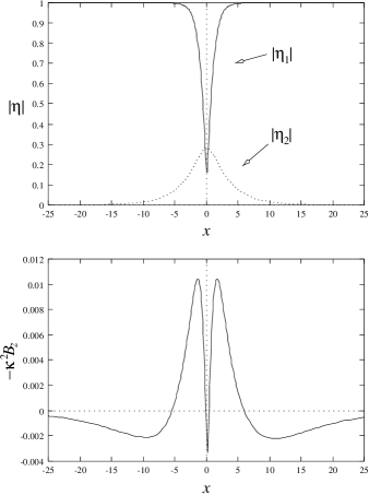
FIG. 3.: Numerical solution of the infinite interface state. Top: The modulus of the two order parameter components. The relative phase is constant $\pi/2$. Bottom: The $z$-component of the magnetic field (multiplied by $\kappa^{2}$). In these units, $\xi_{1}=1$ and $\lambda=7$ ($\kappa^{2}=49$). The magnetic field exhibits variations on the lengthscales $\xi_{1}$ and $\xi_{2}$ in the immediate vicinity of the interface, and is screened away from the interface on the lengthscale $\lambda$.

D Numerical solution for the infinite interface state

Finally we solve the complete set of coupled GL equations for the uniform interface in order to show that our analytic treatment gives the correct qualitative behavior. We choose the coherence length $\xi_{1}=\sqrt{K_{1}/|a_{1}|}$ as the unit length and the London penetration depth about 10 times $\xi_{1}$. For the coefficients we use values of order unity: $a^{\prime}=\beta_{2}=\beta_{1}=K_{2}=K_{1}=1,\tilde{K}=0.1,\gamma=1$ and $\delta=1/4$. The transition temperature of the $d_{xy}$-component is $T_{c2}=0.4T_{c1}$. For the space coordinate we introduce a fine mesh and the interface is taken as single point. For simplicity we consider the symmetric situation by representing the interface via a local suppression of $T_{c1}$: $g_{1}|\eta_{1}|^{2}\delta(x)$.

The solution for $g_{1}=4,g_{2}=0$ is shown in Fig. 3. The shapes of the order parameters (top) are in good qualitative agreement with the analytic result. We see that the length scales $\xi_{1}$ and $\xi_{2}$ are different and that the latter is larger than the former. The relative phase $\theta$ between the two components is constant, $\theta=\pi/2$. The magnetic field has a narrow peak with a width of the order $\xi_{1}$ on the interface (bottom). Towards the bulk, the field changes sign and decays on the length $\lambda$ ($=7\xi_{1}$). The positive and negative parts of the field distribution cancel each other such that no net magnetization is present, as anticipated above.

E Numerical solution for the grain boundary corner

In Sect. II we showed that at the border between two different grain boundary segments with ${\cal T}$-violating states a vortex with fractional flux can appear. We would like to demonstrate this fact here by solving the complete GL problem for a system with a grain boundary which has a corner. For simplicity we use a right angle corner which matches well with our choice for the 2D-square lattice mesh. A variable grid has been introduced to enhance the accuracy in the vicinity of the interface where the order parameter and magnetic field have the largest variations. A steepest descent (relaxation) method was used to minimize the GL free energy with open boundary conditions at the borders of the mesh.

The coefficients of the GL free energy are the same in both grains (see caption of Fig. 5). However, the interface terms for the grain boundary are different for the two segments separated by the corner. The geometry of the grain boundary configuration is shown in Fig. 4. The $A$ and $B$ superconducting regions are separated by the grain boundary, represented as a thick black line. For the segment of the interface parallel to the $x_{A}$- ($y_{A}$-)axis we choose $\tilde{J}_{11}=0.1$, $\tilde{J}_{12}=-(+)0.2$, $\tilde{J}_{21}=-(+)0.2$ and $\tilde{J}_{22}=0.1$. In region $A$, $g_{1}=2.5$ and $g_{2}=0$. In region $B$, $g_{1}=5$ and $g_{2}=0$. As discussed above, the difference in these boundary conditions yields different phase shifts $\alpha$ in the two segments. For the parameters chosen, the phase shifts are equal in magnitude and opposite in sign in the two segments, as expected from Eqs. 6 and 7.

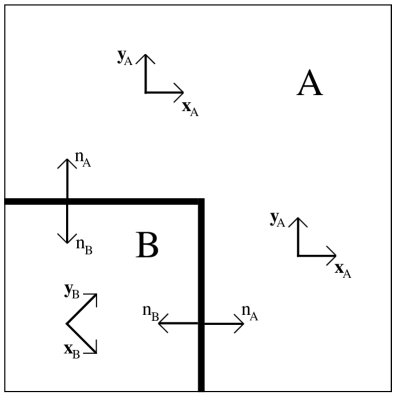
FIG. 4.: Grain boundary configuration used in the calculation of fractional flux. The grain boundary is indicated by the thick line. The $A$ region and $B$ region represent different crystal grains, characterized by their respective principal axis vectors as shown. The normal vectors at each interface are also shown. In the numerical calculation, the density of mesh points is greatest near the grain boundaries.

In Fig. 5 we show the magnetic field distribution around the corner which has a pronounced peak indicating the position of the vortex. The flux is fractional of the size $\Phi\approx-0.15\,\Phi_{0}$. Along the grain boundary the small field peak occurs which we found already for the uniform boundary case. This peak is distorted somewhat by the Josephson coupling of the order parameters across the interface. We also see a slight difference in the decay of the magnetic field towards the grains and along the grain boundaries. The grain boundaries are usually good contacts so that the magnetic flux at the corner is well defined. The sign and magnitude of the flux can be manipulated by tuning $g_{i}$ and $J_{ij}$. Setting all the $J_{ij}$ to 0 eliminates the flux, of course. Switching the signs of $J_{12}$ and $J_{21}$ while leaving $J_{11}$ and $J_{22}$ unchanged reverses the sign of the magnetic flux, as expected from Eqs. 6 and 7. Interestingly, by choosing the $J_{ij}$ and $g_{i}$ appropriately we can favor the formation of a domain wall along the grain boundary at one or both interfaces. The magnetic field distribution along the grain boundary in this case becomes antisymmetric with respect to reflection across the boundary. The parameters chosen for Fig. 5 do not lead to such a domain wall on either interface.

The grain boundaries themselves are naturally good conduits for magnetic flux. In the case shown in Fig. 5, negative magnetic flux pours into the central dip in $B_{z}$ along the interface and drags down the side lobes (Fig. 3, bottom). In general, we expect the grain boundary to pin bulk vortices ($\Phi=\pm n\Phi_{0}$) on top of the fractional vortices due to this tendency to grab magnetic flux. This is consistent with the experimental observations of Kirtley and coworkers [16].

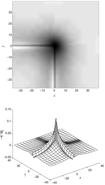
FIG. 5.: The magnetic field distribution at this grain boundary corner. Top: contour plot. Lighter (darker) shades indicate more positive (negative) magnetic fields. Bottom: surface plot of $-\kappa^{2}B_{z}$. The parameters used are $\xi_{1}=1$, $\kappa=7$, $K_{1}=K_{2}=\alpha_{1}=\beta_{1}=\beta_{2}=\gamma=1$, $\delta=1/4$, $\tilde{K}=0.1$, and $\kappa=7$. For the segment of the interface parallel to the $x_{A}$- ($y_{A}$-)axis, $\tilde{J}_{11}=\tilde{J}_{22}=0.1$, $\tilde{J}_{12}=\tilde{J}_{12}=-(+)0.2$. In region $A$, $g_{1}=2.5$ and $g_{2}=0$. In region $B$, $g_{1}=5$ and $g_{2}=0$. The enclosed flux is $\Phi\approx-0.15\,\Phi_{0}$.

IV Conclusions

We have studied the properties of grain boundaries in $d$-wave superconductors. We have demonstrated how they can support a superconducting state with broken time reversal symmetry. We established a connection between such a state and the existence of vortices carrying a fractional flux. The key to this connection lies in the observation that a ${\cal T}$-violating state at the grain boundary can lead to a non-trivial phase shift in the Josephson current-phase relation. Vortices occur at locations where this phase shift changes. Corners of grain boundaries are important places for such vortices, because they separate segments with different properties.

Our results compare qualitatively well with the experimental observation by Kirtley and coworkers [16]. At present it is, however, unclear whether we should consider these experimental results as an evidence for fractional vortices and, consequently, for the presence of a ${\cal T}$-violating superconducting phase. Obviously, if the length scale of the magnetic field along the grain boundary is comparable with the distance between the corners or the vortices, then it is impossible to associate a definite flux with each vortex separately. In order to draw a firm conclusion, this point has to be clarified experimentally.

The conditions for the observation of this effect are best if the crystal orientations of the grains are chosen so that the grain boundary faces a lobe of the $d_{x^{2}-y^{2}}$-wave pair wavefunction on one side and nearly a node on the other. As we pointed out in Sect. III the latter boundary provides a particularly good situation for pair breaking of the $d_{x^{2}-y^{2}}$-wave component, which is an important condition for our scenario. Similar conclusions where found with alternative mechanisms [28, 29]. Unfortunately, grain boundaries of this type are intrinsically difficult to produce as homogeneous interfaces and are often hampered by irregularities.

In conclusion we would like to emphasize that the effect discussed here is a consequence of the exotic nature of the superconducting order parameter. No analoguous effect is possible in the case of a conventional $s$-wave superconductor, because grain boundaries have little effect on this pairing type.

We benefited from discussions with P.A. Lee, Y.B. Kim, K. Kuboki, S. Bahcall and S. Yip. This work was supported in part by NSF Grant No. DMR-9120361-002 and the NSF MRL program through the Center for Materials Research at Stanford Univerity. M. S. gratefully acknowledges a fellowship from Swiss Nationalfonds and financial support from the NSF-MRSEC grant DMR-94-00334.

REFERENCES

- [1] Strongly Correlated Electronic Materials Proceedings of The Los Alamos Symposium 1993, edited by K.S. Bedell, Z. Wang, D.E. Meltzer, A.V. Balatsky and E. Abrahams, Addison Wesley (1994).
- [2] M. Sigrist and T.M. Rice, Z. Phys. B 68, 9 (1987).
- [3] B.G. Levi, Physics Today May 1993, 17 (1993).
- [4] P.B. Littlewood, C.M. Varma, and E. Abrahams, Phys. Rev. Lett. 63, 2602 (1989).
- [5] An alternative scenario was recently introduced by A. Abrikosov, where the occurrence of the node structure in the pair wavefunction is intimately connected with the orthorhombic distortion; A.A. Abrikosov, Physica C 222, 191 (1994); preprint.
- [6] W.N. Hardy et al., Phys. Rev. Lett. 70, 3999 (1993).
- [7] D.J. Scalapino, Physics Reports 250, 329 (1995).
- [8] V.B. Geshkenbein and A.I. Larkin, Pis’ma Zh. Eksp. Teor. Fiz. 43, 306 (1986) [JETP Lett. 43, 395 (1986)]; V.B. Geshkenbein, A.I. Larkin and A. Barone, Phys. Rev. B 36, 235 (1987).
- [9] M. Sigrist and T.M. Rice, J. Phys. Soc. Jpn. 61, 4283 (1992).
- [10] D.A. Wollman et al., Phys. Rev. Lett. 71, 2134 (1993); D. Brawner and H.R. Ott, Phys. Rev. B 50, 6530 (1994); A. Mathai et al., Phys. Rev. Lett. 74, 4523 (1995).
- [11] C.C. Tsuei, J.R. Kirtley, C.C. Chi, L.S. Yu-Jahnes, A. Gupta, T. Shaw, J.Z. Sun and M.B. Ketchen, Phys. Rev. Lett. 73, 593 (1994); J.R. Kirtley, C.C. Tsuei, J.Z. Sun, C.C. Chi, L.S. Yu-Jahnes, A. Gupta, M. Rupp and M.B. Ketchen, Nature 373, 225 (1995).
- [12] P. Chaudhari and S.Y. Lin, Phys. Rev. Lett. 72, 1048 (1994).
- [13] A.J. Millis, Phys. Rev. B 49, 15408 (1994).
- [14] A.G. Sun, D.A. Gajewski, M.B. Maple and R.C. Dynes, Phys. Rev. Lett. 72, 2267 (1994).
- [15] M. Sigrist, K. Kuboki, P.A. Lee, A.J. Millis and T.M. Rice, Phys. Rev. B 53, 2835 (1996).
- [16] J.R. Kirtley, P. Chaudhari, M.B. Ketchen, N. Khare, S.Y. Lin and T. Shaw, Phys. Rev. B 51, 12057 (1995).
- [17] L.P. Gor’kov, Sov. Sci. Rev. A Phys. 9, 1 (1987); M. Sigrist and K. Ueda, Rev. Mod. Phys. 63, 239 (1991).
- [18] C.H. Choi and P. Muzikar, Phys. Rev. B 39, 9664; V.P. Mineev, Pis’ma Zh. Eksp. Teor. Fiz. 49, 624 (1989) [JETP Lett. 49, 719 (1989)]; M. Sigrist, T.M. Rice and K. Ueda, Phys. Rev. Lett. 63, 1727 (1989).
- [19] R.H. Heffner, J.L. Smith, J.O. Willis, P. Birrer, C. Baines, F.N. Gygax, B. Hitti, E. Lippelt, H.R. Ott, A. Schenk, E.A. Knetsch, J. A. Mydosh, and D.E. MacLaughlin, Phys. Rev. Lett. 65, 2816 (1990).
- [20] Q. Dai, J. L. Levy, A. L. Fetter, C. B. Hanna, and R. B. Laughlin, Phys. Rev. B 46, 5642 (1992), and references therein; A. M. Tikofsky, R. B. Laughlin, and Z. Zou, Phys. Rev. Lett. 69, 3670 (1992); A. M. Tikofsky and R.B. Laughlin, Phys. Rev. B 50, 10165 (1994).
- [21] R.B. Laughlin, Physica 234C, 280 (1994).
- [22] G. Kotliar, Phys. Rev. B 37, 3664 (1988).
- [23] S. Spielman et al., Phys. Rev. Lett. 65, 123 (1990); T.W. Lawrence, A. Szöke, and R.B. Laughlin, Phys. Rev. Lett. 69, 1439 (1992); R. Kiefl et al., Phys. Rev. Lett. 64, 2082 (1990).
- [24] S. Kamal, D.A. Bonn, N. Goldenfeld, P.J. Hirschfeld, R. Liang, and W.N. Hardy, Phys. Rev. Lett. 73, 1845 (1994).
- [25] M. Sigrist, D.B. Bailey, and R.B. Laughlin, Phys. Rev. Lett 74, 3249 (1995).
- [26] see, for example, M. Tinkham, Introduction to Superconductivity, McGraw-Hill Book Company (1975).
- [27] M. Sigrist and Y.B. Kim, J. Phys. Soc. Jpn. 63, 4314 (1994).
- [28] S. Yip, Phys. Rev. B 52, 3087 (1995).
- [29] K. Kuboki and M. Sigrist, J. Phys. Soc. Jpn. 65, 361 (1996).