Abstract

We study the thermodynamic behaviour of an ideal gas of bosons trapped in a three-dimensional anisotropic harmonic oscillator potential. The condensate fraction as well as the specific heat is calculated using the Euler-Maclaurin approximation. For a finite number of particles there is no phase transition, but there is a well defined temperature at which the condensation starts. We also consider condensation in lower dimensions, and for one-dimensional systems we discuss the dependence of the condensate fraction and heat capacity on the ensemble used.

1 Introduction

The observation of Bose Einstein condensation (BEC) in ultracold alkali gases has led to intensive experimental and theoretical investigations of the phenomenon [1]. Since the atomic gases of the experiments are dilute, and hence weakly interacting, their physical properties may be explored theoretically in terms of basic interatomic interactions and as a first approximation the interactions may be neglected [2]. This is strongly opposed to the physical properties of related phenomena such as superconductivity in metals and superfluidity in liquid He, which are fundamentally modified by strong interparticle interactions.

In the remarkable pioneering experiment [3] ⁸⁷Rb vapour was magnetically trapped and evaporatively cooled to approximately $170$ nK, where a finite fraction of the particles was observed to occupy the ground state. When further lowering the temperature this fraction increased abruptly, signalling a Bose-Einstein condensation. The confining magnetic field was a time-averaged, orbiting potential [4] whose effective potential to first order is a three-dimensional anisotropic harmonic oscillator. The potential was not anisotropic in all three directions, but was cylindrically symmetric. Shortly after, a similar experiment was performed with ²³Na gas [2]; in this case the potential was completely anisotropic.

With these experiments in mind, we will in the present paper extend our previous work on the thermodynamics of an ideal isotropic gas [5, 6] to the anisotropic case.

Although the interactions among the atoms are weak, they are quite important in the condensate. Both experiments and theory show that due to the interaction the actual ground state is considerably larger than the single particle ground state. However, close to the transition temperature just a few particles occupy the ground state and the gas is much more dilute. At these temperatures one would believe that the ideal gas is a good approximation.

In Ref. [7] it has been proposed that highly anisotropic traps may freeze out one or two dimensions, so that the system to a good approximation is lower dimensional. This implies that it is of interest to study these systems also, and we present a preliminary analysis of them in this work.

The plan of the article is as follows. In the next section we study noninteracting bosons in a confining anisotropic harmonic potential in three dimensions (3$D$). In the framework of the grand canonical ensemble we calculate the condensate fraction, the internal energy and the heat capacity analytically using Euler-Maclaurin summation and compare with exact numerical summation. In section three we discuss the same system in one and two spatial dimensions. In particular, we study the effect of using different ensembles in one-dimensional systems. In section four we summarize and conclude.

2 Bose-Einstein Condensation in Three Dimensions

In this section we will discuss Bose-Einstein condensation in three-dimensional harmonic traps. Firstly, we consider the isotropic potential and then we move on to the anisotropic trap. However, we would first like to discuss Bose-Einstein condensation and phase transitions in a more general setting, and comment upon earlier work.

Let us begin our discussion by considering free bosons in 3$d$ in the thermodynamic limit ($N,V\rightarrow\infty$, $N/V=\rho$ finite). In this case one may show (see any standard textbook in statistical mechanics) that the fraction of particles in the ground state is given by

$$\frac{N_{0}}{N}=1-\Big{(}\frac{T}{T_{c}}\Big{)}^{3/2},$$ (1)

where $T_{c}$ is defined through

$$\rho\left(\frac{2\pi\hbar^{2}}{mk_{B}T_{c}}\right)^{3/2}=\zeta(3/2).$$ (2)

As can be seen from the above equation, $T_{c}$ defines the onset of the condensation of particles into the ground state. Moreover, it can be demonstrated that the chemical potential vanishes for $T\leq T_{c}$ and that $\mu<0$ for $T>T_{c}$. Thus, one can define the critical temperature to be the highest temperature for which $\mu=0$. The derivative of $\mu$ with respect to temperature is discontinuous at $T=T_{c}$, and so there is a first order phase transition.

Generally, the chemical potential must satisfy $\mu\leq E_{0}$, where $E_{0}$ is the ground state energy of the system, in order to have positive occupation numbers. In [8], Kirsten and Toms propose that a necessary criterion for Bose-Einstein condensation is that $\mu$ must reach the ground state energy $E_{0}$ at finite temperature. From this, they show that BEC only occurs for free bosons when $D\geq 3$, and not for free bosons in a finite volume in three dimensions. In a system with a constant magnetic field it only happens in five or more dimensions. This latter result has also been verified independently by Elmfors et al [9].

From theoretical work as well as from an experimental point of view we will argue that this criterion is somewhat too strict. In Ref. [6] it has been demonstrated numerically that the chemical potential never reaches its critical value in the case of bosons in a confining harmonic potential. According to the criterion mentioned above, this system does not exhibit BEC. However, the occupation number of the ground state changes considerably in a narrow temperature range, and attains a macroscopic value. More specifically, it has been shown (see e.g. [6]) that the condensate near $T_{0}=\frac{\hbar\omega}{k_{B}}\Big{(}\frac{N}{\zeta(3)}\Big{)}^{1/3}$ varies as

$$\frac{N_{0}}{N}=1-\Big{(}\frac{T}{T_{0}}\Big{)}^{3}+O(N^{-1/3}).$$ (3)

This abrupt change in number of particles in the ground state takes place near the temperature at which the heat capacity has a pronounced maximum (which is $T_{0}$). We would not hesitate to call this a condensation, although there is no critical behaviour and so it is not obvious how to define a critical temperature. However, in Ref. [10] it has been proposed that the critical temperature is defined by the maximum of the specific heat. According to this criterion there is a phase transition in two and three dimensions, but not in one (see also section three). We think is it natural to call the temperature $T_{0}$ the condensation temperature, since this temperature determines the onset of condensation of particles into the ground state. This view is supported by experiment, namely the fact that one has measured a large increase in the number of particles in the ground state over a narrow temperature region.

2.1 Isotropic Potential

The eigenfunctions of the three-dimensional harmonic oscillator Hamiltonian can always be written as products of three eigenfunctions of the one-dimensional oscillator, which are Hermite polynomials. Hence, the eigenfunctions can be labeled by three integers $n_{x}$, $n_{y}$ and $n_{z}$ and the energy is $\hbar\omega(n_{x}+n_{y}+n_{z})$ in the isotropic case (we have set the ground state energy to zero). Each energy level can thus be characterized by a single quantum number $n$ and the corresponding degeneracy is $g_{n}=(n+1)(n+2)/2$, which simply is the number of ways of writing $n$ as the sum of the three positive integers $n_{x}$, $n_{y}$ and $n_{z}$. The quantum number $n$ then takes the values $n=0,1,2,\ldots$. Due to the high degree of symmetry of the isotropic harmonic well, there is another convenient basis set. The Hamiltonian commutes with $\hat{L}^{2}$ and $\hat{L}_{z}$ and hence the eigenfunctions can be labeled by $L$, $L_{z}$ and the energy. The eigenfunctions are Laguerre polynomials times a spherical harmonic.

At temperature $T$ and chemical potential $\mu$ the particle number $N$ is given by

$$N=\sum_{n=0}^{\infty}\frac{g_{n}}{e^{\beta(\varepsilon_{n}-\mu)}-1},$$ (4)

where $\beta=1/k_{B}T$ and $g_{n}/(e^{\beta(\varepsilon_{n}-\mu)}-1)$ is the usual Bose-Einstein distribution function. Introducing the fugacity $\lambda=\exp(\beta\mu)$, the ground state particle number may be written as

$$N_{0}=\frac{\lambda}{1-\lambda}.$$ (5)

The number of particles in excited states is then

$$N_{e}=\sum_{n=1}^{\infty}\frac{g_{n}\lambda e^{-bn}}{1-\lambda e^{-bn}},$$ (6)

which is a function of the effective fugacity $\bar{\lambda}=\lambda e^{-b}$ where $b=\beta\hbar\omega$.

Since the particle number is given, one must express the chemical potential as a function of temperature and particle number by inverting Eq. (4) in order to derive thermodynamic quantities describing the system. Of particular interest to us is the particle number in the ground state as well as the specific heat of the system as a function of temperature.

Now let us move on to actual calculations and consider different ways of handling Eq. (4). At high temperature $b\ll 1$, the difference between the terms in the sum is small, and one can approximate the sum by an integral. The dominating contribution at high $T$ is found by setting $g_{n}\simeq n^{2}/2$, leading to the semiclassical limit [5, 11]. The transition temperature, as defined by the temperature at which $\lambda=1$, is in this approximation, found to be [5]

$$T_{0}=\frac{\hbar\omega}{k_{B}}\left(\frac{N}{\zeta(3)}\right)^{1/3}.$$ (7)

In the same approximation the specific heat $C_{V}$ exhibits a discontinuity at this temperature with the shape of a $\lambda$. The discontinuity is however an artifact of the approximation. An exact numerical calculation [6] reveals that $C_{V}$ is a continuous function of $T$. This is a consequence of the finiteness of the particle number.

As discussed in [6], an efficient way of performing summations is given by the Euler-Maclaurin summation method [12]. The sum is then written as an integral plus an infinite series of correction terms

$$\sum_{n=a}^{n=b}f(n)=\int_{a}^{b}dxf(x)+\frac{1}{2}[f(b)+f(a)]+\frac{1}{12}[f^{\prime}(b)-f^{\prime}(a)]+\cdots$$ (8)

Applying this formula to the sum over excited states, the contributions from the upper limit vanish (it is natural to single out the ground state from the sum and use Euler-Maclaurin on the rest. Moreover, the series converges much faster doing so). Higher order derivatives mainly bring down higher powers of $\hbar\omega/k_{B}T$, although differentiation of the degeneracy factor yields small corrections to lower order. At high temperature we may therefore safely truncate the series. Including only the first derivative, the number of excited particles becomes

$$N_{e}=G_{3}(\bar{\lambda})+\frac{3}{2}G_{2}(\bar{\lambda})+G_{1}(\bar{\lambda})+\frac{1}{4}\frac{\bar{\lambda}}{1-\bar{\lambda}}\left(\frac{31}{6}+\frac{b}{1-\bar{\lambda}}\right).$$ (9)

We have here introduced the functions

$$G_{p+1}(\bar{\lambda})=\frac{1}{p!}\int_{1}^{\infty}dx\frac{x^{p}\lambda e^{-bx}}{1-\lambda e^{-bx}}.$$ (10)

These functions satisfy a simple recursion relation

$$G_{p+1}(\bar{\lambda})=-\frac{1}{bp!}\ln(1-\bar{\lambda})+\frac{1}{b}\int_{0}^{\bar{\lambda}}\frac{d\lambda}{\lambda}G_{p}(\lambda).$$ (11)

They can be expressed in terms of the more familiar polylogarithmic functions

$$\mbox{Li}_{p}(z)=\sum_{n=1}^{\infty}\frac{z^{n}}{n^{p}},$$ (12)

which are generalizations of the Riemann $\zeta$-function. For $p=0,1,$ and $2$ we have

$$G_{1}(\bar{\lambda}) = \frac{1}{b}\mbox{Li}_{1}(\bar{\lambda})$$

$$G_{2}(\bar{\lambda}) = \frac{1}{b}\mbox{Li}_{1}(\bar{\lambda})+\frac{1}{b^{2}}\mbox{Li}_{2}(\bar{\lambda})$$

$$G_{3}(\bar{\lambda}) = \frac{1}{2b}\mbox{Li}_{1}(\bar{\lambda})+\frac{1}{b^{2}}\mbox{Li}_{2}(\bar{\lambda})+\frac{1}{b^{3}}\mbox{Li}_{3}(\bar{\lambda}).$$ (13)

The Li-functions are obtained when the lower limit of the integral in Eq. (10) is set to zero. For $n\leq 1$ they may be written in terms of more familiar functions, e.g. $\mbox{Li}_{1}(z)=-\ln(1-z),\mbox{Li}_{0}(z)=z/(1-z)$. The polylogarithms satisfy the functional relation

$$\frac{d\mbox{Li}_{p}(z)}{dz}=\frac{1}{z}\mbox{Li}_{p-1}(z).$$ (14)

In terms of these functions, the total number of particles reads

$$N_{e} = \frac{\lambda}{1-\lambda}+\frac{1}{b^{3}}\mbox{Li}_{1}(\bar{\lambda})+\frac{5}{2b^{2}}\mbox{Li}_{2}(\bar{\lambda})+\frac{3}{b}\mbox{Li}_{1}(\bar{\lambda})$$ (15)

$$+ \frac{1}{4}\frac{\bar{\lambda}}{1-\bar{\lambda}}\left(\frac{31}{6}+\frac{b}{1-\bar{\lambda}}\right).$$

The internal energy as well as the heat capacity have been derived in a similar way in Ref. [6].

2.2 Anisotropic Potential

The potentials used in the experiments [2, 3] are either partially or completely asymmetric. We therefore need expressions for the cases where the frequencies are different. Let us first consider the case $\omega_{x}=\omega_{y}\neq\omega_{z}$. As for the isotropic potential we use the Euler-Maclaurin formula for each of the sums. The calculations are similar and we skip the details. The result is

$$N = \frac{\lambda}{1-\lambda}+\frac{1}{b_{x}^{2}b_{z}}\mbox{Li}_{3}(\lambda_{xz})+\left(\frac{1}{2b_{x}^{2}}+\frac{2}{b_{x}b_{z}}\right)\mbox{Li}_{2}(\lambda_{xz})$$ (16)

$$+\left(\frac{b_{z}}{12b_{x}^{2}}+\frac{1}{b_{x}}+\frac{11}{12b_{z}}\right)\mbox{Li}_{1}(\lambda_{xz})+\left(\frac{b_{z}}{6b_{x}}+\frac{11}{24}+\frac{b_{x}}{6b_{z}}\right)\mbox{Li}_{0}(\lambda_{xz})$$

$$+\frac{1}{b_{x}^{2}}\mbox{Li}_{2}(\lambda_{x})+\frac{2}{b_{x}}\mbox{Li}_{1}(\lambda_{x})+\frac{11}{12}\mbox{Li}_{0}(\lambda_{x})$$

$$+\frac{1}{b_{z}}\mbox{Li}_{1}(\lambda_{z})+\frac{1}{2}\mbox{Li}_{0}(\lambda_{z})+{\cal O}(\mbox{Li}_{-1}).$$

We have here introduced the notation $\lambda_{xz}=\lambda\exp(-b_{x}-b_{z})$ etc. where $b_{x}=\hbar\beta\omega_{x}$ and so on. We also need the internal energy and the result using the Euler-Maclaurin formula is

$$U/T = \frac{3}{b_{x}^{2}b_{z}}\mbox{Li}_{4}(\lambda_{xz})+\left(\frac{5}{b_{x}b_{z}}+\frac{2}{b_{x}^{2}}\right)\mbox{Li}_{3}(\lambda_{xz})$$ (17)

$$+ \left(\frac{7b_{z}}{12b_{x}^{2}}+\frac{7}{2b_{x}}+\frac{35}{12b_{z}}\right)\mbox{Li}_{2}(\lambda_{xz})+\left(\frac{b_{z}^{2}}{12b_{x}^{2}}+\frac{5b_{z}}{12b_{x}}+\frac{23}{12}+\frac{17b_{x}}{12b_{z}}\right)\mbox{Li}_{1}(\lambda_{xz})$$

$$+ \left(\frac{b_{z}^{2}}{6b_{x}}+\frac{79b_{z}}{144}+\frac{19b_{x}}{24}-\frac{b_{z}^{3}}{360b_{x}^{2}}+\frac{b_{x}^{2}}{12b_{z}}\right)\mbox{Li}_{0}(\lambda_{xz})$$

$$+ \frac{2}{b_{x}^{2}}\mbox{Li}_{3}(\lambda_{x})+\frac{3}{b_{x}^{2}}\mbox{Li}_{2}(\lambda_{x})+2\mbox{Li}_{1}(\lambda_{x})+\frac{5b_{x}}{4}\mbox{Li}_{0}(\lambda_{x})$$

$$+ \frac{1}{b_{z}}\mbox{Li}_{2}(\lambda_{z})+\mbox{Li}_{1}(\lambda_{z})+\frac{5b_{z}}{12}\mbox{Li}_{0}(\lambda_{z})+{\cal O}(\mbox{Li}_{-1}).$$

The specific heat is now found by differentiating $U$ with respect to $T$. In doing so we need $d\mu/dT-\mu/T$ which is found by differentiation of $N$.

In the ²³Na experiment all three frequencies were different [2]. Thus, we need the expression for the particle number in this case also. By applying the Euler-Maclaurin approximation one finds that $N$ reads

$$N = \frac{\lambda}{1-\lambda}+\frac{1}{b_{x}b_{y}b_{z}}\mbox{Li}_{3}(\lambda_{xyz})+\frac{1}{2}\left(\frac{1}{b_{x}b_{y}}+\mbox{sym.}\right)\mbox{Li}_{2}(\lambda_{xyz})$$ (18)

$$+\frac{1}{4}\left[\frac{1}{b_{x}}+\mbox{sym.}+\frac{1}{3}\left(\frac{b_{x}}{b_{y}b_{z}}+\mbox{sym.}\right)\right]\mbox{Li}_{1}(\lambda_{xyz})$$

$$+\frac{1}{8}\left[1+\frac{1}{3}\left(\frac{b_{x}}{b_{y}}+\mbox{sym.}\right)\right]\mbox{Li}_{0}(\lambda_{xyz})+\frac{1}{b_{x}b_{y}}\mbox{Li}_{2}(\lambda_{xy})$$

$$+\frac{1}{2}\left(\frac{1}{b_{x}}+\frac{1}{b_{y}}\right)\mbox{Li}_{1}(\lambda_{xy})+\frac{1}{4}\left[1+\frac{1}{3}\left(\frac{b_{x}}{b_{y}}+\frac{b_{y}}{b_{x}}\right)\right]\mbox{Li}_{0}(\lambda_{xy})+\mbox{sym.}$$

$$+\frac{1}{b_{x}}\mbox{Li}_{1}(\lambda_{x})+\frac{1}{2}\mbox{Li}_{0}(\lambda_{x})+\mbox{sym.}+{\cal O}(\mbox{Li}_{-1}),$$

Here, “sym.” means symmetrization, e.g.

$$\frac{1}{b_{x}b_{y}}+\mbox{sym.}=\frac{1}{b_{x}b_{y}}+\frac{1}{b_{x}b_{z}}+\frac{1}{b_{y}b_{z}}.$$ (19)

The two leading terms at high temperature are

$$N=\frac{1}{b_{x}b_{y}b_{z}}\mbox{Li}_{3}(\lambda)+\frac{1}{2}\left(\frac{1}{b_{x}b_{y}}+\frac{1}{b_{x}b_{z}}+\frac{1}{b_{y}b_{z}}\right)\mbox{Li}_{2}(\lambda).$$ (20)

In [13] Grossmann and Holthaus considered a potential where $\omega_{y}=\sqrt{2}\omega_{x}$ and $\omega_{z}=\sqrt{3}\omega_{x}$. They constructed a continuous density of states based upon the two leading terms in the degeneracy. For the $\mbox{Li}_{2}$-term they found a coefficient $\gamma(k_{B}T/\hbar\omega)$ where $\omega=(\omega_{x}\omega_{y}\omega_{z})^{1/3}$. A numerical summation gave $\gamma\simeq 1.6$. This numerical factor is now easily found from Eq. (20):

$$\gamma=\left(\frac{3}{4}\right)^{1/3}\left(\frac{1}{\sqrt{2}}+\frac{1}{\sqrt{3}}+\frac{1}{\sqrt{6}}\right)\simeq 1.538,$$ (21)

which agrees quite well with their approximate result. The same value for $\gamma$ has been obtained independently in [14].

For the internal energy one finds

$$U/T = \frac{3}{b_{x}b_{y}b_{z}}\mbox{Li}_{4}(\lambda_{xyz})+2\left(\frac{1}{b_{x}b_{y}}+\mbox{sym.}\right)\mbox{Li}_{3}(\lambda_{xyz})$$ (22)

$$+\frac{1}{4}\left[5\left(\frac{1}{b_{x}}+\mbox{sym.}\right)+\frac{7}{3}\left(\frac{b_{x}}{b_{y}b_{z}}+\mbox{sym.}\right)\right]\mbox{Li}_{2}(\lambda_{xyz})$$

$$+\left[\frac{3}{4}+\frac{b_{x}}{3b_{y}}+\frac{b_{x}^{2}}{12b_{y}b_{z}}+\mbox{sym.}\right]\mbox{Li}_{1}(\lambda_{xyz})$$

$$+\frac{2}{b_{x}b_{y}}\mbox{Li}_{3}(\lambda_{xy})+\frac{3}{2}\left(\frac{1}{b_{x}}+\frac{1}{b_{y}}\right)\mbox{Li}_{2}(\lambda_{xy})$$

$$+\left(1+\frac{b_{x}}{2b_{y}}+\frac{b_{y}}{2b_{x}}\right)\mbox{Li}_{1}(\lambda_{xy})+\mbox{sym.}+\frac{1}{b_{x}}\mbox{Li}_{2}(\lambda_{x})$$

$$+\mbox{Li}_{1}(\lambda_{x})+\mbox{sym.}+{\cal O}(\mbox{Li}_{0}).$$

Again the specific heat can be found by differentiation of this expression.

2.3 Results

With the formulas derived above at hand, we can make predictions for the actual physical systems within the ideal gas approximation. In doing so we have used the values for the oscillator frequencies and particle numbers as given in [2, 3].

For the completely anisotropic system (²³Na) the frequencies are 410, 235 and 745 Hz, and the particle number $N$ is 700 000. The frequencies for the ⁸⁷Rb experiment are $\omega_{z}=240\pi$ Hz and $\omega_{x,y}=\omega_{z}/\sqrt{8}$, and the particle number is 20 000. For these systems we have calculated both the condensate fraction and the specific heat using the Euler-Maclaurin approximation. The results are compared with those of direct numerical summation and the semiclassical approximation. The temperature is measured in units of the semiclassical transition temperature $T_{0}$. It is 1666 nK for the sodium gas and 127 nK for the rubidium gas.

In Fig. 1 we plot the condensate fraction as function of temperature. The numerical and analytical results agree well. For $N=$ 700 000 the transition is quite sharp, and the condensate nearly vanishes about 1% below $T_{0}$. For the smaller particle number, the transition is smoother.

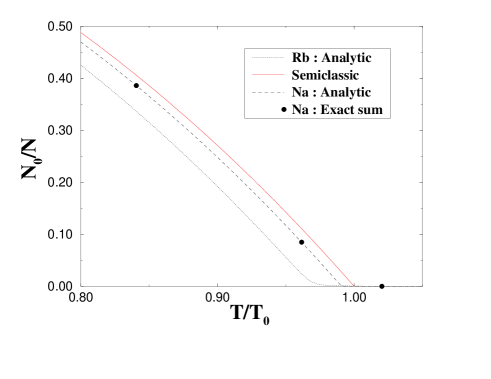
Figure 1: The condensate fraction $N_{0}/N$ in three dimensions with anisotropy-parameters taken from the ²³Na and ⁸⁷Rb experiments. $N_{0}/N$ is plotted as a function of $T/T_{0}$.

The specific heat is shown in Fig. 2. We again find good agreement between numerical and analytical results. The discontinuity in the semiclassical approximation is smoothened by the corrections. Still, for $N=$ 700 000, the specific heat falls rapidly over a temperature range of less than 10 nK. For this case it has a maximum value of $C_{V}/Nk_{B}\simeq 10.43$ , quite close to the semiclassical value $12\zeta(4)/\zeta(3)\simeq 10.80$.

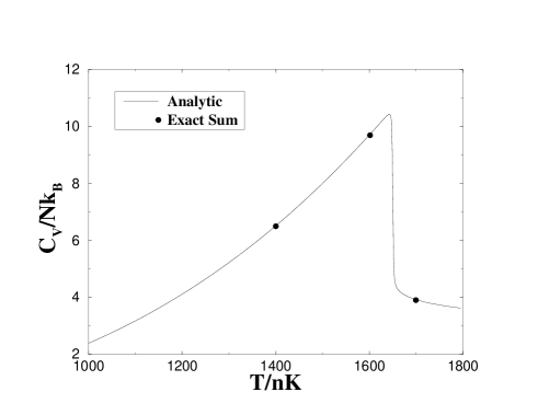
Figure 2: The specific heat $C_{V}$ in an ansiotropic three-dimensional trap with frequencies taken from the ²³Na experiment. $C_{V}$ is plotted as a function of $T/nK$.

3 BEC in Lower Dimensions

All BEC-experiments on trapped Bose gases reported so far are performed on three-dimensional systems. However, by the use of optical dipole traps or highly anisotropic magnetic traps one might, effectively, freeze out oscillations in one or two of the dimensions at low temperatures. In Ref. [7] the authors suggest the use of a field configuration with a radial energy level spacing of 200 nK, and a much smaller axial spacing. At temperatures below 100 nK this system should effectively be one-dimensional.

In the previous section we discussed in some detail different criteria for BEC. The same arguments apply here and we make a few comments. For a free gas in the thermodynamic limit, the chemical potential vanishes first at $T=0$. This implies that the critical temperature in one and two dimensions is zero and that the condensate vanishes at finite temperature. In a finite volume there is again no critical behaviour and there is a condensate even at finite temperature. This is also the case for an ideal gas trapped in an external harmonic potential, as we shall see below.

In this section we consider the trapped Bose gas in both one and two dimensions using the same methods as for three dimensions. We start by examining the case of a highly anisotropic three-dimensional system, and demonstrate the effective reduction to one dimension when two of the oscillator frequencies are much higher than the third. After this, we briefly discuss the use of different ensembles in one dimension. As opposed to two and three dimensions it is here quite straightforward to use the canonical ensemble. For completeness, we also give some results for the two-dimensional case.

3.1 Reduction to One Dimension

Excitations in a given direction of the trap will be suppressed when the temperature is below the energy scale set by the corresponding oscillator strength. The highly anisotropic trap with $\omega_{x,y}\gg\omega_{z}$ should therefore effectively be one-dimensional at temperatures $k_{B}T\ll\hbar\omega_{x,y}$. In Fig. 3 we have plotted the condensate fraction and specific heat $C_{V}$ for the case $\omega_{x,y}=800\omega_{z}$. In the same figure we also give the results for a one-dimensional system with frequency $\omega_{z}$.

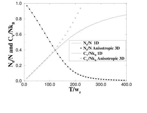
Figure 3: Comparison of the condensate fraction and the specific heat of the highly anisotropic trap and the one-dimensional trap.

The three-dimensional condensate fraction is seen to agree very well with the one-dimensional one at low $T$, but at higher temperatures the former is somewhat reduced due to radial excitations. These excitations have a more dramatic effect on the specific heat. The two curves have high temperature limits of three and one, respectively.

The expressions for the particle number and the energy density in the one-dimensional case are given by:

$$N=\sum_{n=0}^{\infty}\frac{1}{e^{\beta(\varepsilon_{n}-\mu)}-1}=N_{0}+\frac{1}{b}\mbox{Li}_{1}(\bar{\lambda})+\frac{1}{2}\mbox{Li}_{0}(\bar{\lambda})+\frac{b}{12}\mbox{Li}_{-1}(\bar{\lambda}),$$ (23)

$$U=\sum_{n=0}^{\infty}\frac{\varepsilon_{n}}{e^{\beta(\varepsilon_{n}-\mu)}-1}=\omega\left[\frac{1}{b^{2}}\mbox{Li}_{2}(\bar{\lambda})+\frac{1}{b}\mbox{Li}_{1}(\bar{\lambda})+\frac{5}{12}\mbox{Li}_{0}(\bar{\lambda})+\frac{b}{12}\mbox{Li}_{-1}(\bar{\lambda})\right].$$ (24)

This one-dimensional system has earlier been studied by Ketterle and van Druten [7]. For $\beta\omega\ll 1$, they obtained the equation

$$N=N_{0}+\frac{1}{b}\mbox{Li}_{0}(\lambda e^{-\beta\omega/2}).$$ (25)

The contribution from the excited states is similar to the first term in Eq. (23), but has a different effective fugacity. From Eq. (25), Ketterle and van Druten have defined a transition temperature $T_{0}$ by setting $N_{0}=0$ and $\lambda=1$. We then have $N\approx\frac{k_{B}T_{0}}{\hbar\omega}\ln\frac{2k_{B}T_{0}}{\hbar\omega}$. In Fig. 4 we compare various approximations for the density, plotting the condensate fraction as function of temperature for $N=2\cdot 10^{4}$. Including all three terms in Eq. (23), the analytical and numerical results agree to three decimal places. The heat capacity is a smooth function of temperature in the limit $N\rightarrow\infty$, and so there is no phase transition in one dimension.

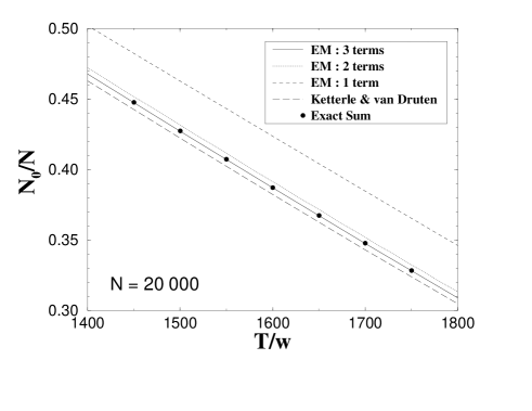
Figure 4: The condensate fraction in different approximations as a function of $T/\omega$. $N=2\cdot 10^{4}$.

3.2 Comparison of Ensembles in One Dimension

The trapped Bose gas has so far been described in terms of the grand canonical ensemble. This implies an open system exchanging energy and particles with a reservoir, where the average particle number is given by the chemical potential.

The experiments are performed at fixed energy and particle number, and should therefore be described in terms of the microcanonical ensemble. The derivation of the corresponding partition function is in general a difficult task, which involves complicated combinatorial problems. Using the canonical ensemble simplifies the calculations considerably, and still satisfies the constraint of fixed particle number.

The different ensembles are known to give the same predictions for thermodynamic quantities in the large $N$ limit [16]. Below we compare the results for the grand canonical and canonical ensembles. The results for the specific heat turn out to agree well. However, for the condensate fraction we find significant deviations.

Assuring that each configuration is counted only once, the partition function in the canonical ensemble can be written as

$$Z=\sum_{n_{1}=0}^{\infty}\cdots\sum_{n_{N}=n_{N-1}}^{\infty}x^{n_{1}+n_{2}+...+n_{N}}=\prod_{i=1}^{N}\frac{1}{1-x^{i}}.$$ (26)

Here, $x=\exp(-\beta\omega)$. The internal energy is now easily found to be

$$U=-\frac{\partial}{\partial\beta}\ln Z=\sum_{i=1}^{N}\frac{i\omega x^{i}}{1-x^{i}},$$ (27)

and the specific heat becomes

$$C_{V}=\frac{\partial U}{\partial T}=\sum_{i=1}^{N}\frac{(i\beta\omega)^{2}x^{i}}{(1-x^{i})^{2}}.$$ (28)

The derivation of the condensate fraction is a little more involved: It can be written as

$$N_{0}=\sum_{k=1}^{N}kp_{k},$$ (29)

where $p_{k}$ is the probability of finding $k$ particles in the lowest energy level. This probability is found summing all contributing configurations:

$$p_{k}=\frac{1}{Z}\sum_{n_{k+1}=1}^{\infty}\cdots\sum_{n_{N}=n_{N-1}}^{\infty}x^{n_{k+1}+n_{k+2}+...+n_{N}}=x^{N-k}\prod_{i=0}^{k-1}(1-x^{N-i}).$$ (30)

In Fig. 5 we have plotted the condensate fraction and the specific heat for $N=10^{3}$ and $N=10^{6}$, as given by the two ensembles. The difference in specific heat is hardly visible for the lower particle number, and for $N=10^{6}$ the results of the two different ensembles agree to six decimal places.

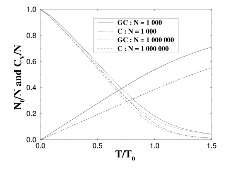
Figure 5: The condensate fraction and the specific heat in different ensembles as a function of $T/T_{0}$ and for different values of $N$.

The situation for the condensate fraction is very different. One can show [17] that the error made calculating $N_{0}$ in the grand canonical ensemble is, at most, of the order ${\cal O}(1/\ln N)$. This is seen from the numerical results given in Fig. 5, where a significant deviation is found at intermediate temperatures even for $N=10^{6}$.

This result is in contrast to the case of a free gas in three dimensions, where the deviation is known to go like $(\ln N)/N$ [18]. A more complete discussion of the finite $N$ effects for this system in the canonical ensemble will be given elsewhere [17].

3.3 Two Dimensions

For completeness we also include results for an isotropic two-dimensional trapped gas. The equation for the particle number here takes the form

$$N=N_{0}+\frac{1}{b^{2}}\mbox{Li}_{2}(\bar{\lambda})+\frac{2}{b}\mbox{Li}_{1}(\bar{\lambda})+\frac{11}{12}\mbox{Li}_{0}(\bar{\lambda})+\frac{b}{6}\mbox{Li}_{-1}(\bar{\lambda}).$$ (31)

The expression for the internal energy reads

$$U=\omega\left[\frac{2}{b^{3}}\mbox{Li}_{3}(\bar{\lambda})+\frac{3}{b^{2}}\mbox{Li}_{2}(\bar{\lambda})+\frac{2}{b}\mbox{Li}_{1}(\bar{\lambda})+\frac{3}{4}\mbox{Li}_{0}(\bar{\lambda})+\frac{b}{6}\mbox{Li}_{-1}(\bar{\lambda})\right].$$ (32)

For large $N$ one may define an approximate condensation temperature setting $N_{0}=0$ and $\lambda=1$. The leading term at high temperature then gives [7]

$$N=\left(\frac{T_{0}}{\omega}\right)^{2}Li_{2}(1)\hskip 28.45274pt\mbox{or}\hskip 28.45274pt\frac{T_{0}}{\omega}=\sqrt{\frac{N}{\zeta(2)}}=\frac{1}{\pi}\sqrt{6N}.$$ (33)

The limiting value at large $N$ for the condensate fraction is

$$\frac{N_{0}}{N}=1-\left(\frac{T}{T_{0}}\right)^{2}.$$ (34)

At temperatures just below $T_{0}$ and large $N$ the energy takes the value $U=2\omega\zeta(3)(T/\omega)^{3}$. This gives a specific heat

$$C_{V}(T\rightarrow T_{0}^{-})=6N\zeta(3)/\zeta(2).$$ (35)

Above $T_{0}$ the leading terms for $C_{V}$ are, again in the large $N$ limit

$$\frac{C_{V}}{N}=6\frac{Li_{3}(\lambda)}{Li_{2}(\lambda)}-4\frac{Li_{2}(\lambda)}{Li_{1}(\lambda)}.$$ (36)

Setting $\lambda=1$, we see that the second term vanishes, and the specific heat approaches the same value as found above. There is thus no jump in the specific heat even in the large $N$ limit in two dimensions.

In Fig. 6 we have plotted the condensate fraction for different values of $N$. The transition sharpens as $N$ grows. The specific heat displayed in Fig. 7 is seen to develop a sharp, though continuous peak with increasing $N$.

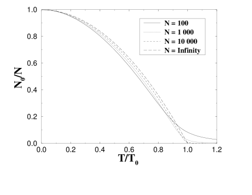
Figure 6: The condensate fraction for different values of the particle number $N$ as a function of $T/T_{0}$.

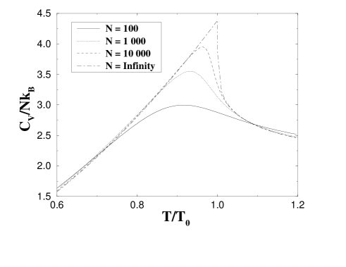
Figure 7: The specific heat for different values of the particle number $N$ as a function of $T/T_{0}$.

This system behaves similarly to the one in three dimensions: The specific heat has a maximum, and the condensate has a powerlike fall off in the large $N$ limit ($N_{0}\sim 1-(T/T_{0})^{2}$ in 2$D$ and $N_{0}\sim 1-(T/T_{0})^{3}$ in 3$D$). Thus, as opposed to the free case, a two-dimensional trapped Bose gas undergoes a phase transition to a condensed state at finite temperature.

4 Conclusions

In the present paper we have discussed the thermodynamics of an ideal Bose gas trapped in an anisotropic harmonic well in some detail. We have investigated the condensate fraction and the heat capacity for realistic values of the frequencies by numerical as well as analytical methods. There is an excellent agreement between the two methods in all dimensions. Moreover, we have studied the highly anisotropic trap where one of the frequencies is much smaller than the others. This system should be realizable in future experiments and it is expected to be effectively one-dimensional for low temperatures. We have therefore compared the condensate and the heat capacity for this system with the corresponding quantities in the one-dimensional trap. The overall agreement for low temperatures confirms the above expectations. We have also considered thermodynamic quantities in different ensembles at finite $N$. The most remarkable result is the deviation of the number of particles in the ground state.

Finally, we would like to mention several possible improvements of the present treatment of BEC. The most obvious is the inclusion of interactions between the atoms in the gas. This could either be based on perturbation theory or some nonperturbative method. There are already a few articles on the subject [19], but more work needs to be done. Secondly, one should use the microcanocial ensemble in order to compare with experiment. It is essentially a combinatorial challenge to do so. More insight into finite $N$ effects of the ideal system is also of interest, and a detailed discussion will be presented in a follow up paper by one of the present authors [17].

References

- [1] http://amo.phy.gasou.edu/bec.html/bibliography.html
- [2] K.B. Davis, M.-O. Mewes, M.R. Andrews, N.J. van Druten, D.S. Durfee, D.M. Kurn, and W. Ketterle, Phys. Rev. Lett. 75, 3969 (1995).
- [3] M. H. Anderson, J. R. Ensher, M. R. Matthews, C. E. Wieman and E. A. Cornell, Science 269, 198 (1995).
- [4] W. Petrich, M. H. Anderson, J. R. Ensher and E. A. Cornell, Phys. Rev. Lett. 74, 3352 (1995).
- [5] H. Haugerud and F. Ravndal, University of Oslo preprint, September 1995, cond-mat/950941.
- [6] H. Haugerud, T. Haugset and F. Ravndal, University of Oslo Preprint TP 4-96, to be published in Phys. Lett. A
- [7] W. Ketterle and N. J. van Druten, Phys. Rev. A 54, 656 (1996).
- [8] K. Kirsten and D. Toms, Phys. Lett. B 368, 119 (1996).
- [9] P. Elmfors, P. Liljenberg, D. Persson, B.-S. Skagerstam, Phys. Lett. B 348, 462 (1995).
- [10] R. K. Pathria, Can. J. Phys. 61, 228 (1983).
- [11] V. Bagnato, D. E. Pritchard and D. Kleppner, Phys. Rev. A 35, 4354 (1987)
- [12] W. H. Press, B. P. Flannery, S. A. Teukolsky and W. T. Vetterling, Numerical Recipes in C, Cambridge University Press (1988).
- [13] S. Grossmann and M. Holthaus, Phys. Lett. A 208, 188 (1995); Zeit. Naturforsch. 50a, 323 (1995).
- [14] K. Kirsten and D. Toms, University of Newcastle Upon Tyne preprint, May 1996.
- [15] W. J. Mullin, cond-mat/9610005.
- [16] R. K. Pathria, Statistical Mechanics, Pergamon Press (1972).
- [17] T. Haugset, in preparation.
- [18] E. H. Hauge, Physica Norvegica 4, 19, (1970).
- [19] See e.g. S. Giorgini, L. Pitaevskii and S. Stringari, cond-mat/9607117; E. Timmerman et al., cond-mat/9609234; H. Shi and W.-M. Zheng, cond-mat/9609241.