Finite–size scaling of the helicity modulus of the two–dimensional O(3) model

Abstract

Using Monte Carlo methods, we compute the finite–size scaling function of the helicity modulus $\Upsilon$ of the two–dimensional O(3) model and compare it to the low temperature expansion prediction. From this, we estimate the range of validity for the leading terms of the low temperature expansion of the finite–size scaling function and for the low temperature expansion of the correlation length. Our results strongly suggest that a Kosterlitz–Thouless transition at a temperature $T>0$ is extremely unlikely in this model.

We report a computation of the finite–size scaling function of the helicity modulus of the two–dimensional O(3) model on the lattice in the presence of periodic boundary conditions. The lattice hamiltonian of the O(3) model is defined as follows:

$${\cal H}=-J\sum_{\langle i,j\rangle}\vec{s}_{i}\cdot\vec{s}_{j},$$ (1)

where the sum runs over nearest neighbors, the pseudospin $\vec{s}=(s_{x},s_{y},s_{z})$ with $s_{x}^{2}+s_{y}^{2}+s_{z}^{2}=1$, and $J>0$ sets the energy scale. The continuum model and its lattice version (1) are supposed to describe the same long wave length physics, i.e. they exhibit asymptotic freedom or in other words, their critical temperature is zero[1, 2, 3]. This is in accord with the Mermin–Wagner theorem[4] which forbids a transition to a state of long range order in a two–dimensional system of O(N) symmetry with N$>1$ at a temperature $T>0$. However, a Kosterlitz–Thouless like transition is still allowed as is well known for the two–dimensional O(2) model[5]. Indeed, there have been arguments in favor of a Kosterlitz–Thouless transition in the two–dimensional O(3) model[6] which have recently been subject to various Monte Carlo investigations[7, 8] focusing on the low temperature behavior of the correlation length. An easily accessible quantity signalling the Kosterlitz–Thouless transition is the helicity modulus. If a Kosterlitz–Thouless transition occurs in the model, on an infinite lattice the helicity modulus exhibits a jump at the transition temperature $T_{c}>0$ from zero to a finite value and remains nonzero for temperatures $T<T_{c}$[9]. However, our result for the finite–size scaling function suggests that the helicity modulus vanishes at all temperatures $T>0$ on infinite lattices, thus a Kosterlitz–Thouless transition is very unlikely to occur in the two–dimensional O(3) model.

We compare our result for the finite–size scaling function to the low temperature expansion prediction of Brézin et al.[10] obtained for the O(3) nonlinear $\sigma$ model and given by

$$\frac{\Upsilon(T,L)}{T}=\frac{1}{2\pi}\left(\ln\frac{\xi_{\Upsilon}(T)}{L}+\ln\ln\frac{\xi_{\Upsilon}(T)}{L}\right)+O(1).$$ (2)

Here $\xi_{\Upsilon}$ denotes a correlation length of the system which behaves as[3]

$$\xi_{\Upsilon}(T)=C_{\Upsilon}(2\pi/T)^{-1}\,\exp(2\pi/T).$$ (3)

The prefactor $C_{\Upsilon}$ cannot be determined within perturbation theory. Note that the scaling form (2) is only valid in the limit $\xi_{\Upsilon}(T)\gg L$.

Numerically we determine the scaling function as follows. We compute the helicity modulus at various temperatures and for different lattice sizes and plot $\Upsilon(T,L)/T$ versus $\ln(LC_{\Upsilon}/\xi_{\Upsilon}(T))$. In the range where the low temperature expansion predictions Eq.(2) and Eq.(3) hold, we expect our scaled data to collapse onto a single curve. Thus, we are able to estimate the range in the variable $z=\ln(LC_{\Upsilon}/\xi_{\Upsilon}(T))$ where the leading behavior (2) sets in and the temperature range where the low temperature expression (3) is valid. For the latter let us assume that the low temperature expansion (3) were not valid above a certain temperature $T_{+}$ say. Then we would see deviations from the scaling curve for values of $z$ larger than $\ln(LC_{\Upsilon}/\xi_{\Upsilon}(T_{+}))$.

For our Monte Carlo simulations, we use the hamiltonian (1) to compute the helicity modulus of the O(3) model on $L\times L$ lattices with $L=10,40,60,100,200$ employing Wolff’s 1–cluster algorithm[11]. In order to avoid boundary effects we apply periodic boundary conditions. Though the leading terms of the scaling expression (2) were derived for fixed spin boundary conditions, the scaling form (2) remains valid for periodic boundary conditions as well. The definition of the helicity modulus along the space direction $\mu$ in the presence of periodic boundary conditions is (for the derivation follow the steps outlined in Refs.[12])

$$\Upsilon_{\mu}(T,L) = \frac{1}{L^{2}}\left\langle\sum_{i}\vec{s}_{i}\cdot\vec{s}_{i+\mu}\right.$$ (4)

$$- \frac{1}{2T}\sum_{[l,m]}\left.\left(\sum_{i}s_{i}^{l}\wedge s_{i+\mu}^{m}\right)^{2}\right\rangle,$$ (5)

$$s_{i}^{l}\wedge s_{i+\mu}^{m} = s_{i}^{l}s_{i+\mu}^{m}-s_{i}^{m}s_{i+\mu}^{l},$$ (6)

where $s^{l}$ and $s^{m}$ denote two different components of the spin $\vec{s}$. The summation is over all possible pairs of spin components, denoted by $\sum_{[l,m]}$, and over all lattice sites, denoted by $\sum_{i}$. The symbol $i+\mu$ means the adjacent lattice site of $i$ in the space direction $\mu$. In the following we will write $\Upsilon$ instead of $\Upsilon_{\mu}$ as our lattice is isotropic. Our definition of the helicity modulus (5) ensures $\lim_{T\rightarrow 0}\Upsilon(T,L)=1$ which agrees with Eq.(2).

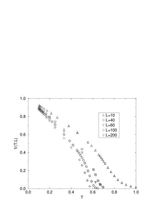
FIG. 1.: The helicity modulus $\Upsilon(T,L)$ as a function of temperature $T$ for various lattices $L\times L$. The error bars are smaller than the symbols.

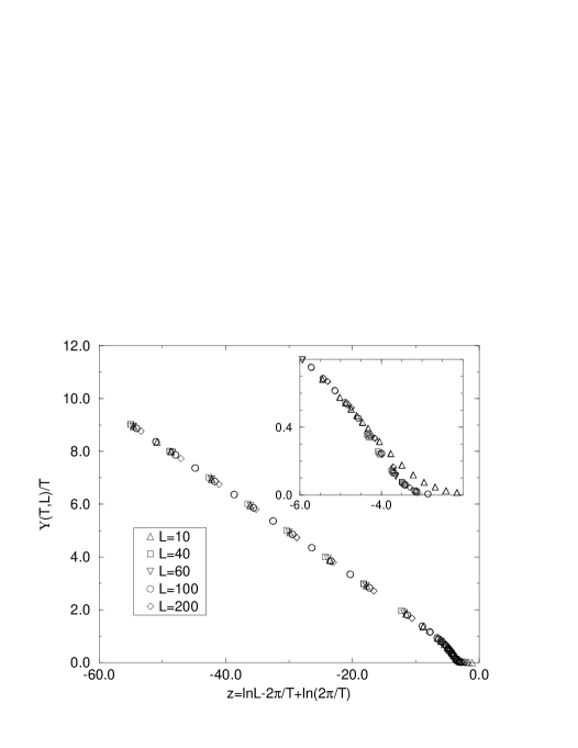
FIG. 2.: Scaling plot $\Upsilon(T,L)/T$ versus $z=\ln L-2\pi/T$ $+\ln(2\pi/T)$. The error bars are smaller than the symbols.

Fig.1 shows our data of the helicity modulus as a function of temperature for various lattice sizes. From this data it is impossible to draw conclusions about the behavior of the helicity modulus of the O(3) model on an infinite lattice. For this reason we have examined the finite–size scaling function in the manner described above.

In Fig.2 we plot $\Upsilon(T,L)/T$ versus $z=\ln L-2\pi/T+\ln(2\pi/T)$ using the data of Fig.1. The data collapse onto a single curve with very little scatter for values $z<-5$, only for $z>-5$ do the data for $\Upsilon(T,10)/T$ begin to deviate from the single scaling curve (cf. the inset of Fig.2), signalling the break down of the expression (3). The corresponding temperature is $T\approx 0.657$, i.e. for temperatures $T$ smaller than $0.657$ the low temperature expansion result (3) should be a good description of the temperature dependence of the correlation length. This temperature is larger than the value $0.37$, obtained in Refs.[7, 13, 14, 15] where the correlation length was computed directly via its second moment definition, and obtained by different methods in Refs.[17].

So far we have only shown that our data of the helicity modulus computed at various temperatures and for different lattice sizes obey scaling. Now we wish to compare the scaled data in Fig.2 with the low temperature prediction Eq.(2). To this end we fit the expression

$$f(z)=a_{1}(a_{2}-z+\ln(a_{2}-z)),$$ (7)

to our scaled data treating $a_{1}$ and $a_{2}=\ln C_{\Upsilon}$ as fit parameters. In principle we should add a constant $a_{3}$ to $f(z)$ to allow for the $O(1)$ term in Eq.(2), however $a_{3}$ turned out to be zero within error bars, therefore we set $a_{3}=0$ for our fits.

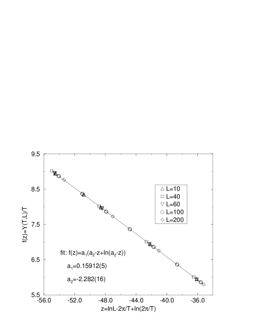
FIG. 3.: Fit of the expression (7) to the scaled data of Fig.2 in the range $-56<z<-35$ (70 data points). The error bars are smaller than the symbols.

data points	$a_{1}$	$a_{2}$	$\chi^{2}$ p.d.f.	$Q$
20	0.1590(4)	-2.23(14)	0.50	0.96
40	0.1592(2)	-2.32(5)	0.64	0.96
60	0.15917(7)	-2.30(2)	0.93	0.63
70	0.15912(5)	-2.28(2)	1.11	0.25
80	0.15905(4)	-2.26(1)	1.09	0.27
100	0.15888(3)	-2.213(6)	1.38	0.0076

TABLE I.: Fitting results of expression (7) to the scaled data shown in Fig.2. $\chi^{2}$ is per degree of freedom and $Q$ is the quality of the fit.

Table I contains our fitting results. We varied the number of data points in the fit to check the stability of our fitting results and to estimate the range of validity of the low temperature result (2) in terms of the variable $z$. We estimate this range from the quality of fit $Q$ (see e.g. Eq.(6.2.18) of Ref.[16]); the closer $Q$ is to 1, the more reliable are the values obtained for the fit parameters $a_{1}$ and $a_{2}$. The value of the parameter $a_{1}$ agrees rather well with the predicted value of $1/(2\pi)=0.15915...$, compare the results of Ref.[18] where the best value $a_{1}=0.162(4)$ was obtained. Fig.3 shows the fitting results of the fit of the form (7) to our scaled data in the range $-56<z<-35$, i.e. including 70 data points.

Since the quality of the fit decreases by an order of magnitude when about 100 data points are included in the fit (cf. Table I), we are on the safe side assuming that formula (2) is valid for values of $z$ in the interval $(-\infty,-35]$ (cf. Fig.3), i.e. expression (2) holds for temperatures and lattice sizes that fulfill

$$\ln\left(\frac{T}{2\pi L}\exp\frac{2\pi}{T}\right)>35.$$ (8)

Our results suggest that the correlation length entering the finite–size scaling form (2) depends on the temperature according to Eq.(3) with $C_{\Upsilon}=0.102$. The prefactor $C_{\Upsilon}$ is about eight times larger than the prefactor $0.0125$[7, 19] obtained from the second moment definition of the correlation length $\xi$[7, 19]. Such a comparatively large prefactor was also found in Ref.[20]. The difference in the prefactors is no surprise to us since we can consider the scaling expression (2) as providing an alternative definition of the correlation length with a prefactor different from that of the second moment definition.

data points	$a_{1}$	$a_{2}$	$\chi^{2}$ p.d.f.	$Q$
20	0.1622(4)	0.6(1)	0.50	0.96
40	0.1626(2)	0.48(5)	0.75	0.87
60	0.16279(7)	0.41(2)	1.12	0.25
70	0.16288(6)	0.39(2)	1.30	0.05

TABLE II.: Fitting results of the expression (9) to the scaled data shown in Fig.2. $\chi^{2}$ is per degree of freedom and $Q$ is the quality of the fit.

We have also fitted the expression

$$f(z)=a_{1}(a_{2}-z),$$ (9)

to our scaled data (the constant $a_{3}$ has been absorbed into $a_{2}$), i.e. neglecting the $\ln\ln$ term in Eq.(2). The results are given in Table II. We find values for $a_{1}$ that differ somewhat from the predicted value of $1/(2\pi)$. Note that as far as the quality of the fit $Q$ (cf. Table II) is concerned, Eq.(9) is as good a description of the scaled data in the range $-56\leq z\leq-35$ as Eq.(7). However, the fit value $a_{1}\approx 0.1626$ does not agree as well with the predicted value [10] $1/(2\pi)$. The inclusion of the $\ln\ln$ correction term yields much better agreement between the value of $a_{1}$ and the universal value $1/(2\pi)$ predicted by the low temperature expansion (2).

Let us conclude with the discussion of the possibility of a Kosterlitz–Thouless transition in the two–dimensional O(3) model. Such a transition has been suggested by Seiler and Patrasciou [6] and its existence has been subject to various Monte Carlo investigations[7, 8]. Since we observe finite–size scaling for the helicity modulus we conclude from our scaled data (cf. Fig.2) that the helicity modulus in the limit of an infinite lattice vanishes at all temperatures. Namely, by fixing the temperature and increasing the lattice size we move along the scaling curve in the direction of increasing $z$ until the helicity modulus vanishes. The existence of a Kosterlitz-Thouless transition, however, would imply a finite value for the helicity modulus below a critical temperature even for an infinite lattice[9]. Our confirmation of the validity of the low temperature expansion together with the strong indication of our scaled data that the helicity modulus on an infinite lattice vanishes, make a Kosterlitz–Thouless transition in the two–dimensional O(3) model extremely unlikely.

In conclusion we have computed numerically the finite–size scaling function of the helicity modulus of the two–dimensional O(3) model and have found very good agreement with the results of the low temperature expansion. We have estimated the ranges of validity of the low temperature expansion in the corresponding variables. Our results suggest that there is no Kosterlitz–Thouless transition in this model.

N.S. would like to thank S. Burnett for valuable discussions.

REFERENCES

- [1] A. M. Polyakov, Phys. Lett. 59B, 79 (1975).
- [2] E. Brézin and J. Zinn–Justin, Phys. Rev. Lett. 36 691 (1976).
- [3] E. Brézin and J. Zinn–Justin, Phys. Rev.B14, 3110 (1976).
- [4] N. D. Mermin and H. Wagner, Phys. Rev. Lett. 17, 1133 (1966).
- [5] J. M. Kosterlitz and D. J. Thouless, J. Phys. C6, 1181 (1973), J. Phys. C7, 1046 (1974).
- [6] A. Patrascioiu and E. Seiler, Nucl. Phys. B (Proc. Suppl.) 30, 184 (1993); A. Patrascioiu and E. Seiler, hep–lat/9508014.
- [7] S. Caracciolo, R. G. Edwards, A. Pelisseto, and A. D. Sokal, Phys. Rev. Lett. 75, 1891 (1995).
- [8] B. Allés, A. Buonanno, and G. Cella, hep–lat/9608002
- [9] D. R. Nelson and J. M. Kosterlitz, Phys. rev. Lett. 39, 1201 (1977); J. V. Jose, L. P. Kadanoff, S. Kirkpatrick, and D. R. Nelson, Phys. Rev. B16, 1217 (1977).
- [10] E. Brézin, E. Korutcheva, Th. Jolicoeur, and J. Zinn–Justin, J. Stat. Phys. 70, 583 (1993).
- [11] U. Wolff, Phys. Rev. Lett. 62, 361 (1989).
- [12] S. Chakravarty, Phys. Rev. Lett. 66, 481 (1990), J. Rudnick and D. Jasnow, Phys. Rev. B16, 2032 (1977).
- [13] P. Hasenfratz and F. Niedermayer, Nucl. Phys. B337 233 (1990).
- [14] U. Wolff, Nucl. Phys. B334 581 (1990).
- [15] J. Apostolakis, C. F. Baillie, and G. C. Fox, Phys. Rev. D43 2687 (1991).
- [16] W. H. Press, B. P. Flannery, S. A. Teukolsky, and W. T. Vetterling, Numerical Recipes (Cambridge University Press, Cambridge, 1988).
- [17] T. Neuhaus, Nucl. Phys. B (Proc. Suppl.) 34, 667 (1994); hep–lat/9608043.
- [18] M. Caffarel, P. Azaria, B. Delamotte, and D. Mouhanna, Europhys. Lett. 26, 493 (1994).
- [19] P. Hasenfratz, M. Maggiore, and F. Niedermayer, Phys. Lett. B245, 522 (1990); P. Hasenfratz and F. Niedermayer, Phys. Lett. B245, 529 (1990).
- [20] A. Billoire, Phys. Rev. B54, 990 (1996).