For: “Mathematics of Materials: Percolation and Composites”, Editors:
 K.M. Golden, G.R. Grimmett, R.D. James, G.W. Milton, and P.N. Sen.
 The IMA Volumes in Mathematics and its Applications (Springer-Verlag, 1997).

SCALING LIMIT FOR THE INCIPIENT SPANNING CLUSTERS

Abstract

Scaling limits of critical percolation models show major differences between low and high dimensional models. The article discusses the formulation of the continuum limit for the former case. A mathematical framework is proposed for the direct description of the limiting continuum theory. The resulting structure is expected to exhibit strict conformal invariance, and facilitate the mathematical discussion of questions related to universality of critical behavior, conformal invariance, and some relations with a number of field theories.

Abstract

AMS(MOS) subject classifications. 82B43, 82B27, 60D05, 82-02

AMS(MOS) subject classifications. 82B43, 82B27, 60D05, 82-02

1 Introduction

Incipient percolation clusters have attracted attention as objects of interesting physical and mathematical properties, and potential for applications. An example of a setup in which they play a role is an array of conducting elements, placed at random in an insulating medium, with the density adjusted to be close to the percolation threshold. In such arrays the current is channelled through fractal-like sets. The concentration of the current, or stress/strain in other similar setups, may result in high amplification of non-linear effects. The phenomenon is of technological interest, and plays a role in high-contrast composite materials and non-linear composites, utilized in thermistors and other devices [1, 2, 3]. Studies of the relevant random geometry have yielded interesting geometric concepts such as the celebrated (but often misunderstood) Incipient Infinite Cluster (IIC). The topic was reviewed from a physics perspective in an article (Stanley [4]) which appeared in Volume 8 of this series, in the proceedings of a workshop held at IMA in 1986.

It is somewhat surprising that percolation threshold phenomena are still a source of delightful and new observations, since the subject seemed to be reaching its maturity already ten years ago. Nevertheless, the subject has recently enjoyed renewed attention; in part because it was realized that some entrenched notions need correction (ref. [5-13]), and in part because it was realized that the scaling (continuum) limit has interesting properties, e.g., conformal invariance, and its construction presents an interesting mathematical challenge [14-16, 10].

This article focuses on issues related to the scaling limit of the Incipient Spanning Clusters (ISC). We discuss a mathematical framework for the direct description of the limiting continuum theory, which is applicable to models below the upper–critical dimension. Within it, we encounter some interesting fractal structures and questions related to: universality of the critical behavior, conformal invariance and relations with certain field theories. The purpose is to describe some recent developments and point directions for possibly interesting progress.

2 The incipient infinite cluster and the incipient spanning clusters

A good starting point for the discussion of the scaling limit is the conceptual difference between two related terms: the Incipient Infinite Cluster (IIC), and the Incipient Spanning Clusters (ISC) (interpreted here as in ref. [12]).

The Incipient Infinite Cluster (IIC) is a thought–provoking notion which has often been used in the discussion of different aspects of critical percolation phenomena ([4]). It has provided a useful and stimulating concept, but one whose different uses have led to some confusion and misinterpretation of theoretical predictions, in particular concerning the question of uniqueness (see the Stauffer paradox discussed in [12]). Consequently, it was recently proposed to differentiate between the two related notions mentioned above: the IIC and the ISC. The distinction is most apparent in the limits in which the two are described by different mathematical entities.

The Incipient Infinite Cluster is a random infinite cluster (or, more completely, a random environment exhibiting an infinite cluster), constructed by a limiting process which provides the “local” picture of the large clusters seen at the percolation threshold — viewed from the perspective of one of their sites. This notion covers three alternative paths which have been explored towards the construction of the IIC:

• Condition on the origin being connected distance $L$ away, and let $L\to\infty$.

• Raise the percolation density above the percolation threshold, condition on the origin belonging to an in infinite cluster, and then let $p\searrow p_{c}$ (where the percolation density presumably vanishes).

• Generate the probability distribution for a random cluster (or a random environment) by centering a typical random configuration relative to one of the sites on its spanning clusters [or just large clusters]. The sampling is to be done with equal weights over all the sites connected to the boundary of $[0,L]^{d}$ (and then let $L\to\infty$), possibly with a corrective exclusion of a boundary zone.

The first two procedures were pointed out by Kesten, who proved their convergence and equivalence in $d=2$ dimensions [17]; the third is more convenient for numerical studies, and was used in [18]. Either way, one may see that the mathematical construction covers the microscopic view of the incipient infinite cluster from the view of one of the rare sites which at $p=p_{c}$ are connected very far – on the microscopic scale. (A somewhat different conception of the IIC is presented in ref [19]. Presumably all will agree in the further scaling/continuum limit).

The Incipient Spanning Clusters, on the other hand, are naturally viewed on the “macroscopic” scale. They are simply the large clusters which reach across the finite sample (in the above example), and connect opposite boundary segments, as indicated in Figure ??. In order to see the entire collection of spanning clusters, we need to keep track of events on the scale of the sample, the relevant limit being: lattice spacing ($\alpha$) $\to 0$.

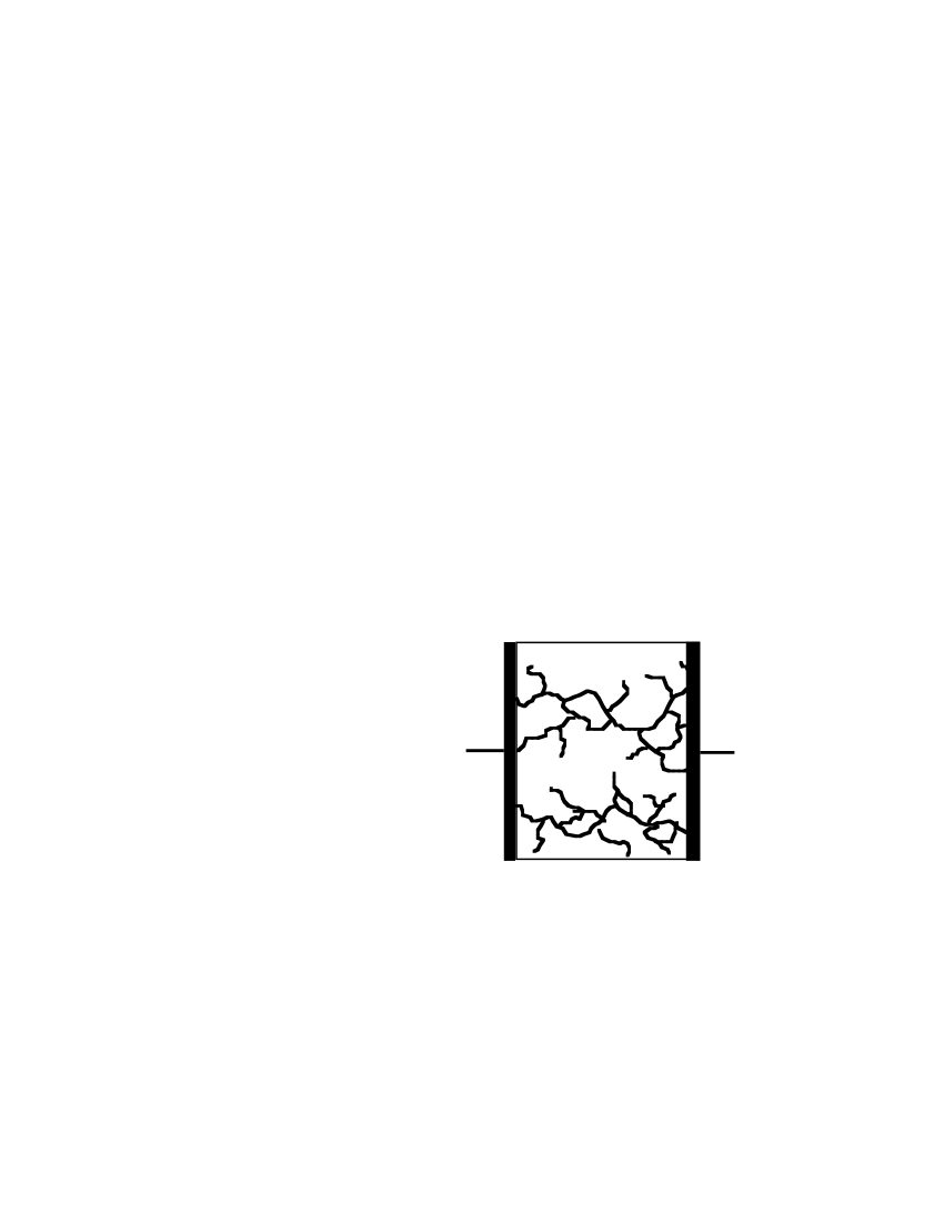
Fig. 1: Incipient Spanning Clusters – a schematic depiction of the the macroscopic view.

A particular difference which stands out, and one which has caused extensive confusion and discussions, is that the the IIC typically shows a single dominant (infinite) cluster, whereas the ISC quite generally exhibit multiple clusters of comparable size, [12]. (A more complete discussion of the related Stauffer paradox is found in ref [12]).

The continuum limit enables a natural discussion of the enhanced symmetry. The highest symmetry emerges at the critical point, for which there is strong evidence of conformal invariance. Considerations related to 2D conformal fields have led to proposals for differential equations which determine some of the properties of the critical measure ([15, 16]). Thus, the continuum limit of the spanning clusters may remind one of the Brownian motion: an object arising from physics, with fascinating mathematical properties, high degree of symmetry, and relation to interesting differential equations.

While we focus here on ICS, similar considerations can be applied to the entire collection of the connected clusters which are visible on the macroscopic scale. The entire ensemble’s scaling limit has been termed the percolation web [12].

3 The microscopic view; three convenient models

There is a variety of situations in which conducting elements are placed at random in an insulating medium. These elements may conduct electric current, or may serve as passages for a liquid seeping through a solid. The individual resistors, or cracks, are visible on the Microscopic Scale. Their relative density is our (dimensionless) control parameter. Following are three convenient models, which offer different advantages as possible starting points for the construction of a (common?) continuum limit.

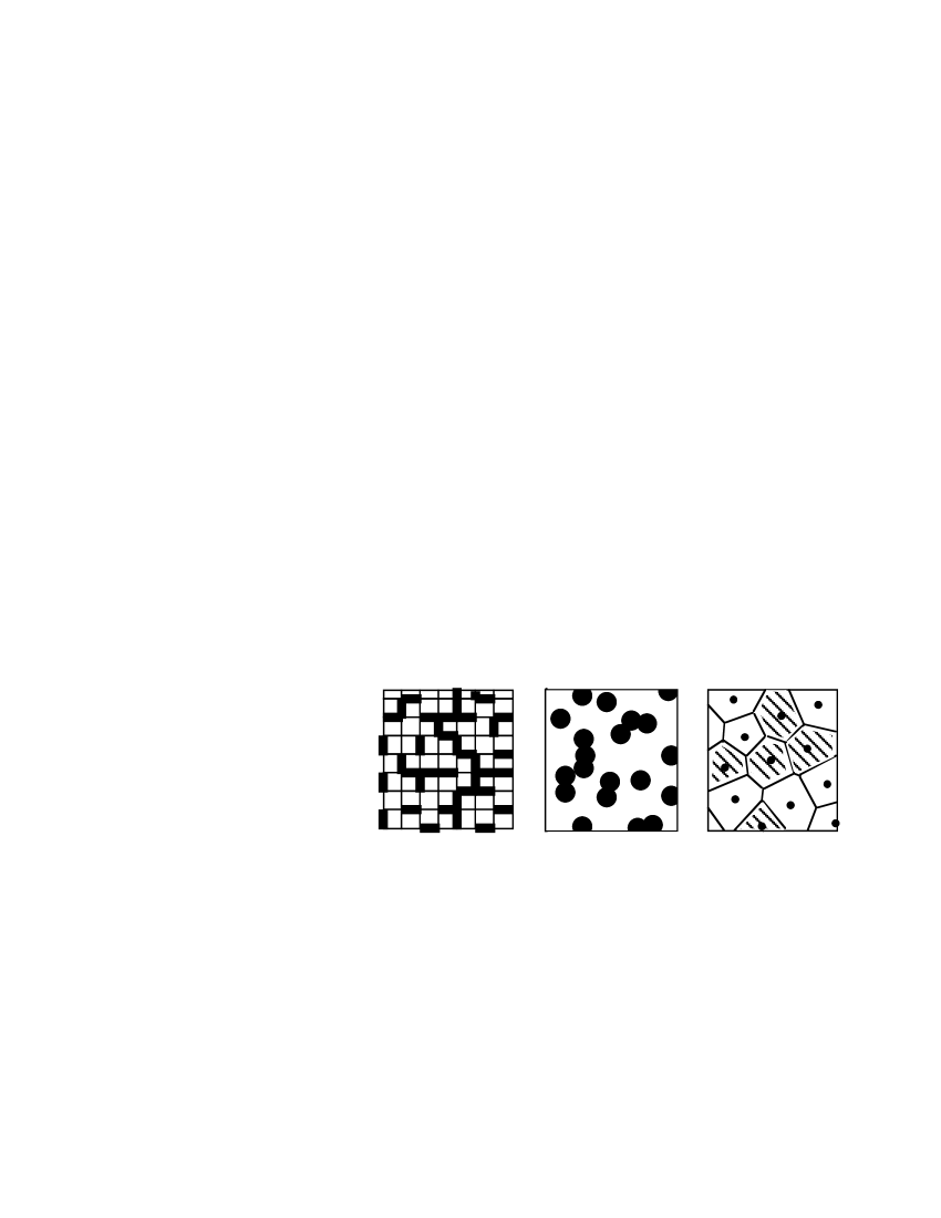
Fig. 2: The microscopic view; different possibilities for the short–distance structure.

Bond-percolation. The model is formulated on the lattice $\alpha Z^{d}$. The randomness is associated with the bonds (pairs of neighboring lattice sites), which are occupied at random, independently with probability $0\leq p\leq 1$ (the control parameter). The occupied bonds are regarded as connecting. They may also represent conductors of conductance $\sigma>0$.

When a bond is not occupied, its dual obstructing object can be regarded as realized. That leads to the self-duality of bond percolation on $Z^{2}$, which is helpful ([20, 21]). In three dimensions, the dual model is that of random plaquettes, which may form encapsulating surfaces obstructing the connections ([22]).

Droplet percolation. This models is formulated over the continuum. The conducting regions consist of randomly distributed d-dimensional balls of radius $\alpha$ (Poisson process, with possible overlaps), with density $\rho d^{d}x$ for the centers of the conducting cells. The relevant dimensionless control parameter is proportional to the density of the conducting regime:

$$p\ =\ \rho\ \alpha^{d}\ .{}$$ (3.1)

The 2D bond model is self dual, while the droplet model is rotation invariant. The following model exhibits both features (a fact noticed independently also by Benjamini and Schramm ([23]), and it, therefore, is our favored starting point for the construction of the purportedly common scaling limit.

Voronoi-tessellation percolation. Starting from a randomly generated configuration of points in $R^{d}$, described by a Poisson process with density $\rho d^{d}x$, the plane is partitioned into the cells of the corresponding Voronoi tessellation. The cells are conducting, or not, independently with probabilities $\{p,1-p\}$. Alternatively stated, two discrete random sets ($A,B\subset R^{d}$) are generated with Poisson densities $p\rho d^{d}x$ and $(1-p)\rho d^{d}x$, and the conducting regime consists of those sites of the continuum which are closer to A than to B. The short-distance scale in this model, $\alpha$, is related to $\rho$ as in eq. ?? (it is of the order of the mean diameter of the Voronoi cells). In two dimensions the model is self-dual, and the critical value for $p$ is $p_{c}=1/2$.

An generalization we shall mention in Section ?? consists of models with a density profile of the form $\rho_{t}(x)d^{d}x$ with $\rho_{t}(x)=t\cdot g(x)$, $g(x)$ continuous and positive. Letting $t\to\infty$ we find a scaling limit for which the density profile shows persistent inhomogeneity on the macroscopic scale. However, since the inhomogeneity corresponds to just different rates of approach towards a common limit, we expect it to have no visible effect on the continuum limit considered here.

Planarity is a very helpful property even without strict self duality. Using it one can prove more for 2D models, at or near $p_{c}$ ([21, 24]), than what is known about other dimensions $2<d<6$, and in particular about $d=3$.

4 The macroscopic perspective

The focus of our discussion is on the geometric features which are visible on the Macroscopic Scale in a systems whose short scale structure is any of the above. Correspondingly, we chose the scale for our discussion so that the object occupies a fixed continuum–scale region $\Lambda_{1}=[-1,1]^{d}$, or more generally $\Lambda_{\ell}=[-\ell,\ell]\times[-1,1]^{d-1}$, and we let the short distance scale be $\alpha<<1$, eventually taken to $0$.

When the sample is placed between two conducting plates, with different electric potentials applied to the two opposite faces:

$$\partial\Lambda_{-}=\{\underline{x}\in\partial\Lambda\ :\ x_{1}=-\ell\}\ ,\ \ \partial\Lambda_{+}=\{\underline{x}\in\partial\Lambda\ :\ x_{1}=\ell\}\ ,$$ (4.1)

we would naturally be interested in the spanning clusters, which are the (maximal) connected clusters linking $\partial\Lambda_{-}$ with $\partial\Lambda_{+}$.

While the changes on the microscopic scale are gradual, at the percolation threshold a drastic transition is observed on the macroscopic scale, where the following is seen with probability which tends to $1$ as $\alpha\to 0$ (for suitably chosen constants $Const.$):

  $p<p_{c}\Rightarrow$

there are no spanning clusters; the diameters of the connected clusters do not exceed $Const.\ \alpha|\log\alpha|$.

  $p>p_{c}\Rightarrow$

there is a unique spanning cluster, which covers the region
“densely”: its spherical voids are all smaller than $Const.\ \alpha|\log\alpha|$.

At the critical point we find:

$p=p_{c}\Rightarrow$

• the spanning probability does not vanish, at least for $\ell<1/2$ (the restriction is not needed for $2D$, otherwise it reflects just a limitation of the existent proof),
  

• for each $0<s<1$ –

$$Prob_{p_{c},a}\left(\begin{array}[]{l}\mbox{the inner region $[-s,s]^{d}$ is connected}\\ \mbox{to the boundary $\partial\Lambda$}\end{array}\right)\ \geq\ C_{d}\ s^{(d-1)/2}$$ (4.4)

(4.5)

• where the bound is uniform in $\alpha$ (!),
  

• there is positive probability for more than one spanning clus-
  ter in $\Lambda$.

Remarks: The proofs of the above assertions are based on a number of different results, some of which were presented most completely for the lattice – rather than continuum, models. The behavior at $p<p_{c}$ follows from the exponential decay of the two point function in the subcritical regime ([25, 26]), the bound on the voids in the percolating phase uses the coincidence of the critical point with the limit of the slab/quadrant percolation thresholds ([27, 28]), as explained in [12]. The statements concerning $p=p_{c}$ in arbitrary dimensions are proven in [12]. The picture described there fits well in the axiomatic description of the critical regime proposed in ref. [29]. The non-uniqueness of the spanning clusters in the two–dimensional case has been familiar to those following the rigorous arguments since the work of Russo [30] and Seymour and Welsh [30, 31], but it became appreciated in some of the physics community only rather recently [11, 13].

Many (though not all ) of the features of the scaling limits of critical percolation are expected to be shared by systems which differ on the microscopic scale. However, beyond the general description presented above, the behavior at $p=p_{c}$ exhibits interesting dimension dependence.

5 Type I and type II critical models

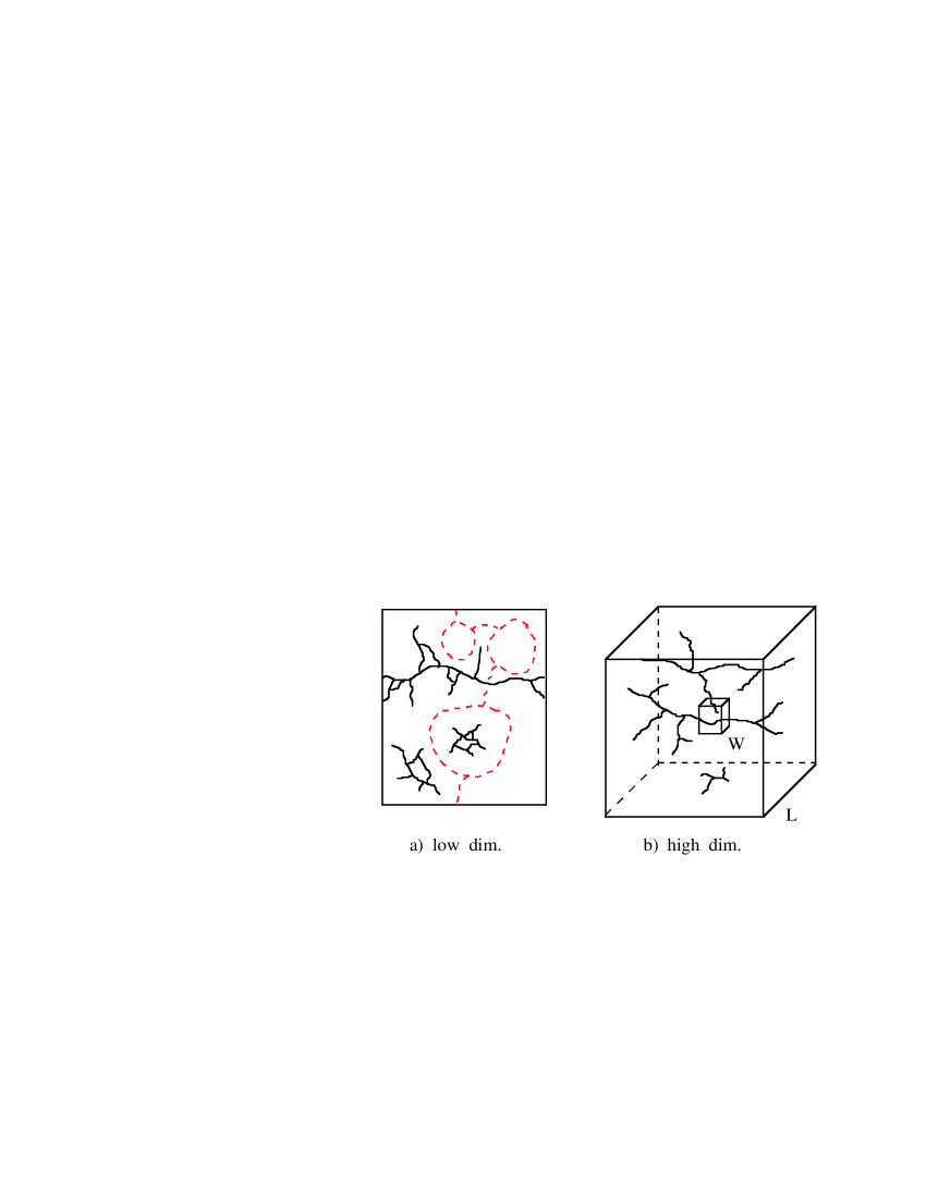
Fig. 3: Two different types of critical behavior (schematically): I) In $2D$ one sees only a finite number of clusters of the size of the volume, typically none of the clusters intersecting a given cube reaches far beyond it – on the corresponding scale, and in the scaling limit the spanning clusters are nowhere dense. II) In high dimensions ($d>6\ ?$) spanning clusters proliferate $(O(L^{d-6}))$ and extend increasing distances. While individual spanning clusters behave as $D=4$ dimensional trees, their union becomes dense in the scaling limit.

The critical behavior is better understood in dimensions $d=2$, and $d>d_{u.c.}$ where $d_{u.c.}$ is the upper–critical dimension whose value for percolation is apparently $d_{u.c.}=6$ ([33-37]). It was, however, recently realized that two cases differ in ways which have pronounced effects on the basic structure of the continuum limits.

In $d=2$ dimensions, the “Russo–Seymour–Welsh theory” [30, 31] (conveniently summarized in [38]) can be used to deduce that:

• A typical configuration has only finitely many spanning clusters – in the sense that

$$Prob_{p_{c},\alpha}\left(\mbox{there are in $\Lambda$ $n$ distinct spanning clusters}\right)\ \leq\ K(n)\ ,$$

(5.1)

uniformly in $0<\alpha\leq 1$, with $K(n)\to 0$ (for $n\to\infty$). More explicitly, $K(n)$ was recently shown to be bounded above $(C)$ and below $(C^{\prime})$ by $A\ e^{-C[C`]\ n^{2}}$, [12].

• Any given internal site in $\Lambda$ is typically surrounded on an infinite sequence of scales ($2^{-n}$; $n=k_{1},k_{2},\ldots$) by “dual circuits” which separate it from all the spanning clusters, and in the limit $\alpha\to 0$ from all clusters whose size remains visible on the macroscopic scale. Of course, exceptions to the rule are found along the spanning clusters, which form random “fractal” sets of lower dimension ($<d=2$).

In contrast, for dimensions $d>6$ under an additional assumption, that $\eta=0$ (as predicted by physical theory [34] which has been supported by the partial rigorous results [36, 39]), we find the following behavior [12]:

• the number of spanning clusters grows, typically, as $a^{-(d-6)}$ (as predicted in ref. [40])

• the spanning probability tends to $1$ and, furthermore, for any fixed open set $B\subset\Lambda$ the probability that a spanning cluster intersects $B$ tends to $1$

• the diameter of the maximal cluster intersecting a given open set, of fixed size on the macroscopic scale ($[-s,s]^{d}$), diverges as $\alpha\to 0$, typically being at least as large as $s^{(d-4)/2}\cdot\alpha^{-(d-6-o(1))/2}$.

One could add that in the latter case the clusters have predominantly tree characteristics, and behave as $D=4$ dimensional objects, as was first suggested in ref. [41, 42].

The above examples, and the results presented below, motivate the distinction which was made in ref. [12] between the following two types of critical behavior.

Type I models: The function

$$\limsup_{\alpha\to 0}\ Prob_{p_{c},\alpha}\left(\begin{array}[]{l}\mbox{the set $[-s,s]^{d}$ is connected}\\ \mbox{to the boundary of $[-1,1]^{d}$}\end{array}\right)\ \ \ =$$ (5.4)

$$\limsup_{\alpha\to 0}Prob_{p_{c},\alpha}\left(\begin{array}[]{l}\mbox{the set $[-1,1]^{d}$ is connected}\\ \mbox{to the boundary of $[-1/s,1/s]^{d}$}\end{array}\right)\ = \tilde{h}(s)$$ (5.7)

is strictly less than one, for some $s<1$. This implies $\lim_{s\to\infty}\tilde{h}(s)=0$, which means that there is no percolation in the scaling limit.

Type II models:

$$Prob_{p_{c},\alpha}\left(\begin{array}[]{l}\mbox{the set $[-s,s]^{d}$ is connected}\\ \mbox{to the boundary of $[-1,1]^{d}$}\end{array}\right)\parbox[t]{28.90755pt}{$\longrightarrow\\ {\scriptstyle\alpha\to 0}$}1\ ,{}$$ (5.8)

for any $0<s<1$.

Remarks: 1) Presumably all other behavior is ruled out for the models considered here, but that was not proven.
2) The function $\tilde{h}(s)$ is obviously submultiplicative, i.e., satisfies $\tilde{h}(s_{1}\cdot s_{2})\ \leq\ \tilde{h}(s_{1})\tilde{h}(s_{2})$ for $0<s_{1},s_{2}<1$. Standard arguments imply the existence of the limit, and its positivity for Type I systems:

$$\lim_{s\searrow 0}\frac{\log\tilde{h}(s)}{\log s}\ =\ \lambda\ >\ 0\ .{}$$ (5.9)

In other words, in Type I critical models $\tilde{h}(s)\ =\ s^{\lambda+o(1)}$ for $s\to 0$, with some $\lambda>0$. In terms of the standard, though not yet fully proven picture [4], the exponent $\lambda$ is related to the Hausdorff dimension of the Incipient Spanning Cluster (or of the ISC), $d_{w}$, as:

$$\lambda\ =\ d-d_{w}\ .$$ (5.10)

In this article we shall not discuss the scaling limit of models of of Type II (i.e., the case $d>d_{u.c.}$). Not that this would be uninteresting: Hara and Slade proposed (as mentioned in [43]) that the limit for individual clusters is related with the Integrated SuperBrownian Excursion process (ISE) of Aldous [44]. Furthermore, looking at the ensemble of all the macroscopic scale cluster we find that in a sense which still has to be made explicit (the one presently in mind is a very weak one) one may anticipate two surprising features: percolation at the critical point, and infinity of infinite clusters [12].

Remark: The above observation may alarm those familiar with lattice percolation models, but the apparent conflict with the general uniqueness Theorems [45, 46] is not a real contradiction; the general result of Burton–Keane [46] requires discreteness on some short–scale.

Our discussion of the scaling limit continues now in the generality of of Type I models. This covers the case of $2D$, and presumably applies also to dimensions $d=3,4,5$ – though there are no rigorous results to support such claim. We of course limit now our attention to the critical regime.

6 Formulation of the scaling limit; type I models

6.1 The question

The quantitative description of the continuum limit is expressed through a number of functions. Two examples are described in Figure ??. The pictures drawn there refer to events defined on the macroscopic scale, with the probabilities considered in the limit $\alpha\to 0$.

Fig. 4: Two functions associated with the continuum limit ($\alpha=$ (lattice spacing) $\to 0$) of Type I critical models: 1) $F$ is the limit of the probabilities that boundary segments are connected as indicated, 2) $G$ is the limit of probabilities that the neighborhoods of the points {$x_{1},x_{2},x_{3}$} are connected.

The question we shall address next is what mathematical object would capture, in a natural way, those geometric features of the Incipient Spanning Clusters which are visible in the scaling limit. This can be rephrased as asking what stochastic–geometric object embedded in $R^{d}$ can be associated with the functions referred to above, and others of this kind, so that they can be naturally viewed as the connectivity probabilities (and not just limits of …).

In the absence of a direct insight a canonical approach could be to to define the object by the list of its quantifiers, and introduce on the space of those some minimal $\sigma$ - algebra which would allow to bring in probabilistic notions. However, as the example of the Wiener process (Brownian motion) shows, it may be worthwhile to learn the regularity properties of the geometric object under consideration.

6.2 The first attempt: ISC as a subset of $\Lambda$

At first sight, it seems natural to regard the ISC as closed subsets of the region $\Lambda\subset R^{d}$. However, this formulation will not serve our purpose.

Before dismissing this attempt, let us recall that what makes the collection of closed subsets of $\Lambda\subset R^{d}$ into a particularly convenient space for the description of random fractals ([47]) is the following classical result.

Theorem 1

For any compact metric space $\Lambda$, the space

$${\mathcal{H}}(\Lambda)=\{A\subset\Lambda:\mbox{\rm\ A is closed }\}$$ (6.1)

is compact in the corresponding Hausdorff metric.

The Hausdorff metric $h(A,B)$ is defined so that $h(A,B)\leq\epsilon$ if and only if $dist(x,B)\leq\epsilon$ for any $x\in A$, and $dist(y,A)\leq\epsilon$ for any $y\in B$.

Alas, the features which are of interest to us, such as the existence and location of connecting paths, are not continuous in the Hausdorff metric. Moreover, the configurations of critical percolation models are typically among the points of discontinuity. The reason is that in typical configurations there are “choke points” where a small-scale change, possibly of a single bond, or cell, would drastically alter the available connecting paths (as indicated in Figure ??a, and more explicitly in Figure 1d of ref. [12]). Such a change shifts the point in ${\mathcal{H}}(\Lambda)$ only a distance of the order $O(\alpha)$, which is not detectable in the scaling limit. However, the effect on the available connecting paths is clearly visible on the large scale.

6.3 Hölder continuity of the connecting paths

Since the scaling limit of the set does not capture the information on the realized connections, it is natural to include that information explicitly in the description of limit. Some of it is expressed through the collection of the realized self-avoiding paths, each given by a continuous function $g:[0,1]\to\Lambda$. In the terminology of [4], we are including both the backbone (BB) paths and the paths connecting the dangling ends to the backbone.

Potential obstacles in describing the configuration through the realized paths are:

• The possibility that as the short scale is refined the connecting paths could become increasingly irregular. It is not a-priori obvious that in the limit $\alpha\to 0$ the connections can still be expressed through continuous functions. (One could worry here about the need to consider more general continua [connected closed sets]. Their collection is somewhat unwieldy, e.g., some continua do not support the image of any continuous non-constant function.)

• It is not initially clear whether the information provided by the set of the connected paths suffices for questions concerning higher order connections. If not, then one might need to list also connected line graphs of higher complexity.

The first concern is completely answered by the following result [48, 49] (see Note Added in Proof, next page).

Theorem 2

For any critical Type I percolation model all the realized connected (self- avoiding) paths in a compact region $\Lambda\subset R^{n}$ can be simultaneously parameterized by uniformly continuous functions, $\underline{g}(t)\ \ 0\leq t\leq 1$, satisfying the Hölder continuity condition:

$$\frac{|\underline{g}(t_{1})-\underline{g}(t_{2})|}{|t_{1}-t_{2}|^{\lambda}}\ \leq\ \kappa(\omega)\ ,\ \ \mbox{for all \ $0\leq t_{1},t_{2}\leq 1$}\ ,$$ (6.2)

with some fixed $0<\lambda<1/d$ and a configuration dependent continuity modulus for which

$$Prob_{p_{c},\alpha}\left(\kappa(\omega)\geq t\right)\ \leq \ g(t)$$ (6.3)

$$\rightarrow 0\ \ \ ,\mbox{ for $t\to\infty$ }$$

uniformly in $\alpha$.

In other words: in Type I models, in the critical regime one seldom finds a connected path in $\Lambda$ which cannot be “traced” in a unit of time by means of a “fairly regular” function. The continuity condition we use is consistent even with a “fractal” landscape, and consequently the regularity does not deteriorate as $\alpha\to 0$. (That is not true for $p>p_{c}$.)

The self–avoidance condition is applied only on the microscopic scale, and should be interpreted in the sense which is natural for the model, e.g., for bond percolation the paths should not repeat any bond, and for the random Voronoi–tessellation the paths should not re–enter any cell. We note that the paths need not appear self–avoiding when viewed on the macroscopic scale (in the limit $\alpha\to 0$).

Concerning the second of the above reservations, the question has a simple answer in $d=2$ dimensions, though the situation in higher $d$ is still not as clearly resolved. The basic issue is: how to determine if a pair of paths which on the scale of the continuum seem to intersect are actually connected on the microscopic scale. As we discussed, there are situations in which two connected paths come within distance $\alpha$ without touching and without there being another path linking the two. Conveniently, at least in $d=2$ dimensions such close encounters 1st kind do not occur at non-terminal points, in the sense which is stated precisely in ref. [12], and proven in ref. [48].

6.4 Our choice: ISC as a collection of realized Hölder–
continuous paths

To formulate the limiting representation of the Backbone and the Incipient Spanning Clusters, we find it convenient to first represent the percolation configuration by the random collection of all the realized (connected) paths in $\Lambda$ which are regular and self-avoiding in the sense explained above. That random object, which we call the percolation Web ($W$, or $W(\omega)$), is of the form

$$W\subset C_{1/d}([0,1],R^{d})\;,$$ (6.4)

where $C_{1/d}([0,1],R^{d})$ is the space of Hölder–continuous functions:

$$C_{1/d}([0,1],R^{d})=\left\{g\in C([0,1],R^{d})\ {:}\sup_{0\leq t_{1},t_{2}\leq 1}\frac{|\underline{g}(t_{1})-\underline{g}(t_{2})|}{|t_{1}-t_{2}|^{1/d}}<\infty\right\}$$

(6.5)

We shall also denote by $W_{\Lambda}(\omega)$ the restriction of $W(\omega)$ to functions with range in $\Lambda\subset\mathtt{R}^{d}$ (i.e. to $C([0,1],\Lambda)$).

In $d=2$ dimensions, the range of values of $W(\omega)$ is constrained by the following consistency conditions, of which the first three are obvious, but the fourth one reflects a non-trivial fact (there [typically] are no close encounters of the $1$st kind, in the limit $\alpha\to 0$).

Percolation web consistency conditions

• (Closure) $W_{\Lambda}(\omega)$ is closed as a subset of $C([0,1],\Lambda)$.

• (Reparametrization–invariance) For each realized path $f\in W_{\Lambda}(\omega)$ any path of the form $\tilde{f}(t)=f(\tau(t))$, with $\tau(\cdot)$ continuous and of bounded derivative [or just a Lipschitz function], is also realized.

• (Splicing stability) If two paths of $W_{\Lambda}(\omega)$ intersect at non-terminal points, then the paths obtained by different “splicings” of the four resulting segments are also realized.

We denote by $\Omega_{\Lambda}$ the collection of subsets of $C([0,1],\Lambda)$ satisfying the consistency conditions C1 – C3.

(Trying not to be too formalistic here, let us just note that $\Omega=\Omega_{R^{d}}$ is a complete separable metric space. The continuum limit of critical percolation models in a macroscopic region $\Lambda$ will be described by probability measures on the natural $\sigma$ algebra on $\Omega(\Lambda)$.)

The Backbone can now be described by the collections of paths in the Web which traverse $\Lambda$,

$$B_{\Lambda}(\omega)=\left\{f\in W_{\Lambda}(\omega):g_{1}(0)=-\ell,\;\;g_{1}(1)=\ell\right\}$$ (6.6)

and the collection of the Incipient Spanning Clusters is described by a collection of pairs of paths, of the form:

$$S_{\Lambda}(\omega)=\left\{(f,g){\Big{|}}\begin{array}[]{l}\mbox{$f\in W_{\Lambda}(\omega),\;\;g\in B(\omega)$, \ with}\\ \mbox{$\underline{f}(0)=\underline{g}(t)$ for some and $0\leq t\leq 1$ }\end{array}\right\}\ \ ,$$ (6.7)

where $(f,g)\in S_{\Lambda}(\omega)$ is taken to imply that there is an actual contact between the paths (at the microscopic level, which is otherwise no longer visible).

7 The web — an existence result

From the perspective of the continuum limit, the microscopic model is a construction scaffold. When it is removed, a more remarkable structure is exposed (as in Emily Dickinson’s metaphor).

Once we have a direct way to formulate the continuum theory, it is mathematically natural to restart the discussion and pose the question in the standard existence and uniqueness terms. It should be appreciated that a successful formulation of the uniqueness question will shed light on the phenomenon of universality in critical behavior.

Following is an existence result [48].

Theorem 3

For each dimension in which the critical behavior is Type I, there is a one–parameter family of probability measures ($\mu$) on $\Omega$ which have the following properties.

• (Independence) For disjoint closed regions, $A\subset B\subset R^{d}$, $W_{A}(\omega)$ and $W_{B}(\omega)$ are independent [as random variables].

• (Euclidean invariance) The probability measure is invariant under translations and rotations.

• (Regularity) The spanning probabilities of compact rectangular regions are neither $0$ nor $1$:

$$R_{s}:=Prob{[\mu]}\left(\begin{array}[]{c}\mbox{there is in $[-s,s]^{d}$ a }\\ \mbox{left $\leftrightarrow$ right spanning cluster}\end{array}\right)\ \ \stackrel{{\scriptstyle\textstyle>\;0}}{{{}_{{}_{\textstyle<\;1}}}}$$ (7.1)

A convenient parametrization within the family of measures is the crossing probability $R_{1}$.

The measures are constructed as continuum limits of sequences of models with suitably adjusted percolation densities. If the standard picture is correct, the density needs be adjusted with the lattice spacing as:

$$p\ =\ p_{c}+(R_{1}-1/2)\ Const.\ \alpha^{1/\nu}\ .$$ (7.2)

In order to end with a rotation invariant measure, we start from either the droplet percolation model, or the Voronoi-tessellation percolation model.

Some open problems:

  Convergence –

A characteristic shortcoming of the available methods is the lack of proof of convergence of the scaling limit. Our construction relies on compactness arguments, which guarantee convergence along subsequences. Proof of convergence will be an outstanding technical contribution to the subject. Alternatively stated, this is a question of uniqueness of the scaling limit.

  Uniqueness –

A broader formulation of the uniqueness question is:
do the three conditions seen in the existence result, Theorem ??, limit the range to only the one–parameter family of measures?
If not, are there additional assumptions which would?
Also: is the full rotation invariance of such measures implied by just the rotation invariance of the cube–crossing probabilities?

Since the measures in question include all the continuum limits of critical percolation models, positive answer would cast in a clear mathematical form some of the expected universality of critical behavior – in a sense which was clearly articulated only relatively recently, in Langlands et.al. [5] and related works [15, 6-9].

Other mathematical challenges are to affirm (or test) the Renormalization Group picture, which suggests some exact properties for the constructed measures, and establish the conjectured conformal invariance of the critical measure (a special member of the one-parameter family).

8 Relation with the renormalization group

The continuum object constructed in Theorem ?? bears an interesting relation to the RG picture. While still no sensible formalism has been found for an exact representation of the renormalization group transformation as a map, the one–parameter family of measures presented in Theorem ?? may be viewed as corresponding exactly to what would be the unstable (i.e., expanding) fiber extending from the critical point in such a space. Along this fiber, the RG maps coincide with dilatations.

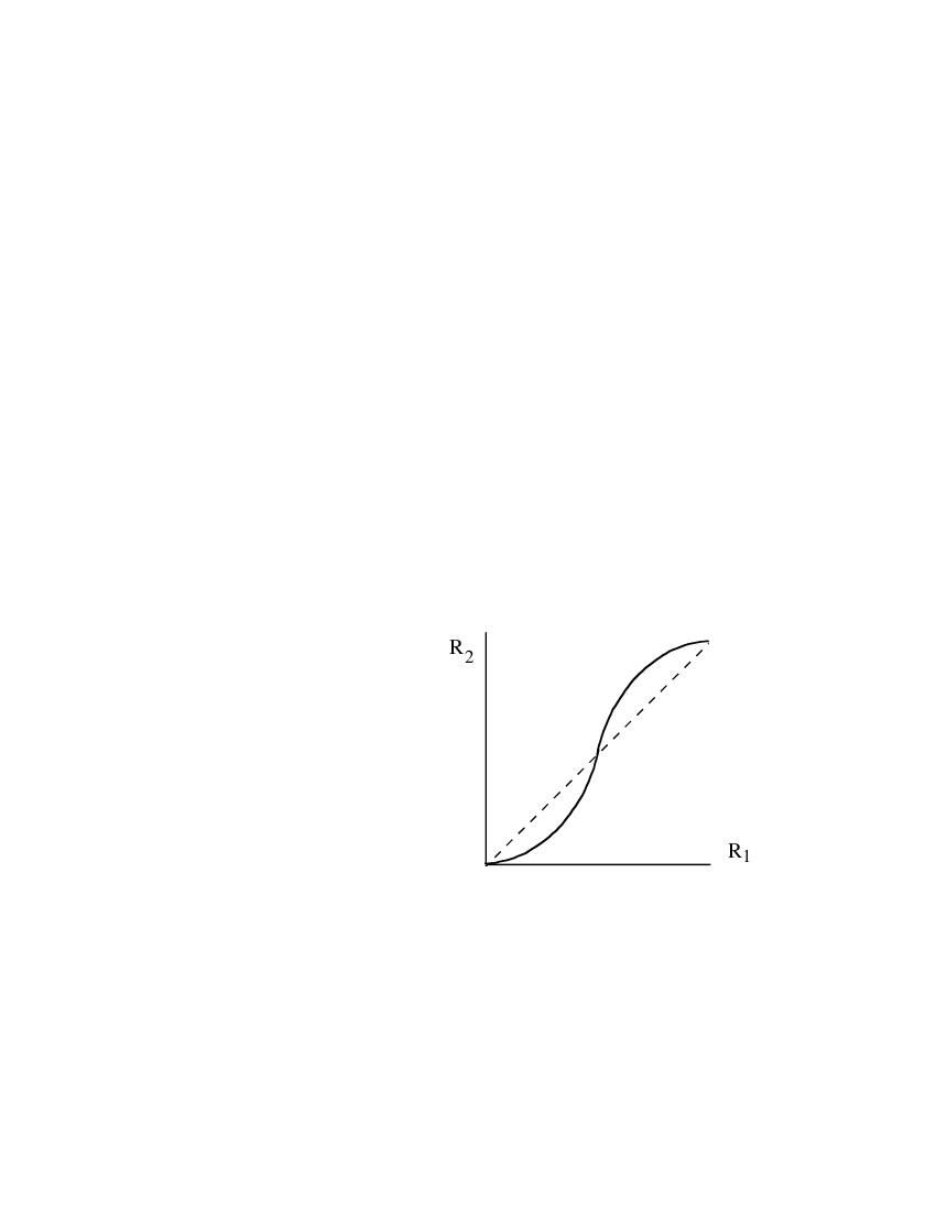
Fig. 5: The conjectured relation between two crossing probabilities in the one-parameter family of the constructed measures (schematically). The map this function generates on $[0,1]$ corresponds to the action of the Renormalization Group along the expanding fiber. Assuming the standard RG picture, the slope of the function at its middle [unstable] fixed point is exactly $2^{1/\nu}$, $\nu$ being the correlation–length critical exponent.

It is interesting to plot the joint values of $R(s)$ and $R(1)$ (say, for $s=2$). The standard RG picture leads us to expect there the $S$-shape of a function which as a map of the unit interval into itself has one unstable fixed point and two stable fixed points at $0$ and $1$ (as in Figure ??). The slope of the function at the unstable fixed point should be exactly $s^{1/\nu}$. (For $2D$ the predicted value is $\nu=4/3$, den Nijs [50]).

Even in the absence of an exact setup, the renormalization group picture has provided very effective approximate tools [51]. One may view Figure ?? as presenting a limit of the “cell to cell” renormalization group map, which recently became appreciated as one of the more effective approximate RG methods [6, 52, 53].

9 Fractal structure

In Type I models, the number of clusters connecting the boundary of a cube $\Lambda\subset R^{d}$, centered at $0$, with the contracted cube $s\Lambda$, $0<s<1$, is finite; in the sense that the probability for observing $k$ such clusters obeys bounds which are uniform in the short–distance/lattice–spacing $\alpha$ (as $\alpha\to 0$), and decay to zero for $k\to\infty$. Correspondingly, the scaling limit exhibits (a.s.) only a finite number of such clusters (once one knows how to count them), and altogether only countably many macroscopic size clusters in $\Lambda$ (the infinity is caused by the union over all scales). Furthermore, the number of “left $\leftrightarrow$ right” spanning clusters remains finite in the continuum limit.

Details of the expected fractal structure were discussed in the review article of Stanley [4] in the context of lattice models. New considerations are added when one looks at the scaling limit. To present some basic results, let us start with–

Definition: 1. For a given configuration of the percolation Web, $W_{\Lambda}(\omega)$, we say that two sites, $x,y\in\Lambda$ are connected if $W_{\Lambda}(\omega)$ includes a path visiting each of them.

2. The connected cluster of a site $x\in\Lambda$ is the union of the sites $y\in\Lambda$ connected to it. We denote it ${\mathcal{C}}(x)={\mathcal{C}}_{\omega}(x)$.

3. ${\mathcal{C}}(\partial\Lambda)$ is the collection of sites connected (as in 1.) to the boundary $\partial\Lambda$.

4. The ramification number $R_{\omega}(x)$ is the maximal value of $k$ for which there are $k$ paths in $W(\omega)$ starting at $x$ and otherwise non-intersecting.

There are some surprises: first is the lack of transitivity of the relation “$x$ is connected to $y$”. We view this not as a shortcoming of the terminology, but rather as an expression of an interesting phenomenon, related to the existence of tenuous connections (when a pivotal bond is reversed, one obtains a configuration in which two realized paths meet without being connected on the microscopic level, an example is indicated in Figure ??a).

The second “surprise” is the first statement in the following list of properties of the scaling limit, ref. [48].

Theorem 4

For Type I critical models, in typical realizations of the percolation Web:

1. The connected clusters of (Lebesgue-)almost all sites $x\in\Lambda$ contain no other site, i.e. $R(x)=0$ or

$${\mathcal{C}}(x)=\{x\}\ .{}$$ (9.1)

2. The collection of sites violating eq. (??), which includes the random set ${\mathcal{C}}_{\omega}(\partial\lambda)$, is of Hausdorff dimension $\leq(d-\lambda)$ (as defined by eq. (??). Furthermore,

3. The above set is of finite ramification; there is a non-random value $k<\infty$ such that $R_{\omega}(x)\leq k$ for all (not just a.e.) $x\in\Lambda$.

For $2D$, we guess that the maximal ramification number is about $k=5$, though that is still not fully resolved.

10 Conjectured conformal invariance

The particular measure which corresponds to the fixed–point value of $R_{1}$ is expected to be fully dilatation invariant. It is conjectured that it is also strictly covariant under conformal maps.

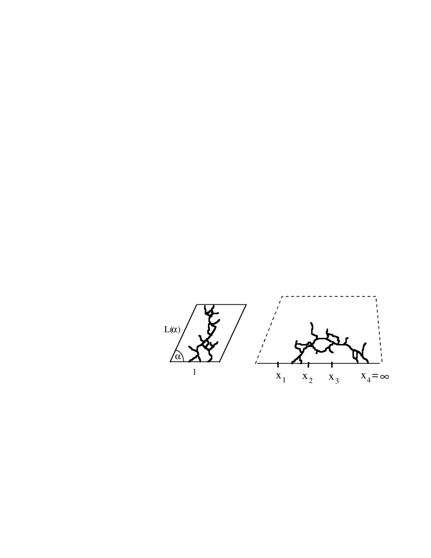
Fig. 6: The setup for the question of Langlands et al. [5] and Cardy’s surmise.

The conformal invariance is expected in any dimension, but the conformal group is particularly large in $2D$ and it is there that the related considerations have been shown to have powerful consequences, and have led to explicit predictions concerning critical behavior in a rich collection of models [54, 55]. For the rest of this section we restrict the attention to two dimensional systems.

The $2D$ scaling limit was studied numerically by Langlands et.al.
(LPPS) [5]. In addition to testing the universality of the spanning probabilities (in a sense which broke new grounds [6, 7, 8, 9]), LPPS asked how should the aspect ratio of a parallelogram be adjusted with the angle (see Figure ??), if one wants to keep the spanning probability constant. This author’s suggestion that the criterion should be conformal equivalence fitted well with the numerical data. A much more complete answer was proposed by J. Cardy [15], who produced a differential equation for the upper–half–plane version of the problem (to which the original one is reduced via the corresponding Riemann map). Cardy’s equation for the crossing probability has a unique solution with the natural boundary conditions, and the resulting function of the angle $\alpha$ and the length $L$ (see Figure ??) was found to be in perfect agreement with the numerical results of LPPS.

Cardy’s equation drew on a field–theoretic perspective, and on an extrapolation based on relations with some other models of Statistical Mechanics. Other insights followed, including Pinson’s proposal [56] for the exact values of the probabilities of different windings for twisted boundary conditions. The reader is referred to [16] for an account of these developments.

The bottom–up derivation of the conformal invariance is still an open challenge. There are some partial results, such as the following one (whose proof is not that difficult) which is conditioned on a strong assumption about the scaling limit.

The result stated below follows [48], but we note that a related statement with a somewhat different formulation was presented in [23] ([the two were arrived at independently]). To formulate the proven assertion, let us first present a statement which upon some consideration appears believable, though its proof has still eluded us.

Conjecture: The Voronoi-tessellation percolation models with position–dependent density profiles of the form $\rho(x)=t\cdot g(x)$, with $g(\cdot)$ continuous and non–vanishing in $\Lambda\subset R^{2}$, the limit $t\to\infty$ exist (for the ISC and for the Web processes), and is independent of the function $g(\cdot)$.

Theorem 5

In $d=2$ dimensions, under the above conjecture and assuming also the critical behavior is Type I, the scaling limit of the Voronoi percolation model is conformally invariant, in the sense that for any map $T\ :\ \Lambda\rightarrow R^{2}$ which is invertible and conformal on $\Lambda$, the image of the ISC [Web] process in $\Lambda$ coincides with the ISC [Web] process in $T\Lambda$.

A particular expression of the conformal invariance is that the function defined in Figure ?? satisfies

$$F_{D}(\{\gamma_{1},\ldots,\gamma_{k}\})\ =\ F_{TD}(\{\gamma_{1},\ldots,\gamma_{k}\})\ ,$$ (10.1)

where $\{\gamma_{1},\ldots,\gamma_{k}\}$ refers to a collection of boundary segments which are to be connected by a common cluster. (One may of course generate a large number of other, similar, functions.)

One may employ also the Riemann map which takes the interior of $D$ conformally onto the upper–half–plane; Figure ?? indicates two such events for which conformal invariance implies equality of probability. In case the boundary of $D$ consists of four segments, conformal invariance implies that the probability depends only on one cross–ratio, i.e., is given by a function of the form

$$f(x_{1},\ldots,x_{4})=\phi(\ u(x_{1},\ldots,x_{4})\ )\ ,{}$$ (10.2)

with

$$u(x_{1},\ldots,x_{4})\ =\ \frac{(x_{1}-x_{2})(x_{3}-x_{4})}{(x_{1}-x_{3})(x_{2}-x_{4})}\ .$$ (10.3)

11 Cardy’s equation

The equation which Cardy proposed for the above quantity can be transcribed as [15, 16]:

$$u(1-u)\frac{d^{2}\phi}{du\mbox{ }^{2}}+\frac{2}{3}(1-2u)\frac{d\phi}{du}\ =\ 0\ ,$$ (11.1)

with the boundary values $\phi(0)=0$, $\phi(1)=1$. The solution can be presented in the integral form:

$$\phi(u)\ =\ \int_{0}^{u}\frac{d\ x}{[x(1-x)]^{2/3}}\ /\ Norm.{}$$ (11.2)

Some algebraic aspects of Cardy’s equation are more visible when it is expressed in terms of the differential operators:

$${\mathcal{L}}_{n}\ =\ -\sum_{j\neq 1}\left(x_{j}-x_{1}\right)^{n+1}\frac{\partial}{\partial x_{j}}\ .$$ (11.3)

In terms of these, the equation (as originally presented) is

$$\left({\mathcal{L}}_{-2}-{\textstyle\frac{3}{2}}{\mathcal{L}}_{-1}^{2}\right)f(x_{1},\ldots,x_{4})\ =\ 0\ .{}$$ (11.4)

Cardy’s original argument [15] invoked an analogy with equations describing the effects on the free energy of certain Potts models of changes in the boundary conditions. Various step in this approach are still beyond the reach of rigorous methods. Let us, however, point out that the very intuitive hypothesis of invariance under conformal maps which preserve the relevant domain (plus the necessary differentiability) implies:

$${\mathcal{L}}_{1}\left({\mathcal{L}}_{-2}-{\textstyle\frac{3}{2}}{\mathcal{L}}_{-1}^{2}\right)f(x_{1},\ldots,x_{4})\ =\ 0\ .{}$$ (11.5)

The derivation of this equation is an elementary and amusing exercise in the Virasoro algebra, of the commutation relations:

$$\left[{\mathcal{L}}_{n},{\mathcal{L}}_{m}\right]\ =\ (n-m)\ {\mathcal{L}}_{n+m}\ ,{}$$ (11.6)

starting from the observation that the conformal invariance assumption implies

$${\mathcal{L}}_{0}f(\ldots)\ =\ 0\ \ ,\mbox{and}\ \ {\mathcal{L}}_{1}f(\ldots)\ =\ 0\ .{}$$ (11.7)

Equation (??) holds since the two operators generate flows preserving $f(\ldots)$, being associated with Möbius transformations which preserve the upper–half–plane and the point $x_{1}$ (${\mathcal{L}}_{-1}$, however, corresponds to a shift of $x_{2},\ldots$ which leaves $x_{1}$ behind). Thus, when the two factors in eq. (??) are transposed $f(\ldots)$ is annihilated by ${\mathcal{L}}_{1}$. The commutator of the two terms is a combination of ${\mathcal{L}}_{0}$, ${\mathcal{L}}_{1}$ and a term proportional to ${\mathcal{L}}_{-1}$ which is eliminated through the judicious choice of the coefficient $3/2$ in eq. (??).

The transition from eq. (??) to eq. (??) amounts to the removal of the former’s leftmost factor. That is however a big step, since it transforms an equation with limited content into one which completely determines the solution. (Although one should not be too dismissive of eq. (??): in terms of the conformal invariance structures, it conveys the fact that for the percolation problem the conformal charge is zero, which is a speculation born out by the Russo–Seymour–Welsh theory [30, 31].)

Though we are still short of a proof, it turns out that one may explain from the Continuum Percolation Web’s perspective a mechanism for the extraction of Cardy’s equation, eq. (??), from eq. (??). The argument employs a plausible description of an effect caused by the separation of scales ([48]).

12 Selected characteristic exponents

Fig. 7: Some characteristic exponents associated with spanning probabilities in $2D$. Solid lines indicate spanning clusters, and dotted lines indicate spanning dual, separating, clusters. Example a) is implied by Cardy’s equation, b) and c) are based on more elementary observations, [21, 48].

An interesting aspect of the explicit solution, eq. (??), is that it yields the power $\epsilon^{1/3}$ for the probability that a short interval, of size $\epsilon$, is connected in the half plane a distance of order $1$ away. This exponent does not appear to be obvious to the naked eye. In Figure ?? we present it next to two other characteristic exponents which have a more elementary derivation (discussed along with other examples and applications in ref. [21, 10, 48]).

Less one would be lulled by the simplicity of the exponents seen in Figure ??, let us mention that the probability of a full annulus to be spanned is predicted to behave as $(r/R)^{5/48}$, den Nijs [50].

Question: What are the values of the characteristic exponents for $k$ disjoint spanning clusters, in the full or cut annulus, for all the other values of $k$?

The exact answer may be within the reach of the methods of Conformal Field Theory [55, 15], or the Coulomb–gas representation, [57], which has been recently discussed by T. Spencer[58]. It was recently proven by other methods that for large $k$ the exponent is of the order of $Const.\ k^{2}$, [12].

13 Relation with field theory

The continuum object described here in earlier sections is related to a number of “field theories”. Cardy’s equation for the function $F$ drew on its analogy with the vacuum expectation value of a product of operators switching the boundary conditions (in Potts models). Another field theoretical object is related with the function $G$, also defined in Figure ??. Its simplest manifestation is in the one–point function defined next.

In the scaling limit of a Type I model, the probability that a given site $x\in D$ is connected to the boundary of the domain $D$ is zero, but the probability that a small ball around it, $B(x,\epsilon)=$ $\{y\ :\ |y-x|\leq\epsilon\}$, is connected to $\partial D$ is positive. Based on the ideas mentioned in Section 5, one expects that for a suitable $d_{w}$ the following limit exists

$$\ \ \ \ h_{D}(x)\ =\ \lim_{\epsilon\to 0}\ \epsilon^{-k(2-d_{w})}\ Prob\left(\mbox{$B(x,\epsilon)$ is connected to $\partial D$}\right)\ .{}$$ (13.1)

If so, and if the probability measure maps covariantly under conformal maps, then, for any conformal transformation $T\ :D\to\mathtt{R}^{d}$

$$h_{D}(x)\ =\ (|\det(\partial T/\partial x)|^{1/d})^{2-d_{w}}\ h_{TD}(Tx)\ .$$ (13.2)

The function $h_{D}(x)$ can be viewed as the expectation value of an entity defined by the limit

$$\psi_{D}(z)\ =\ \texttt{w}-\lim_{\epsilon\to 0}\ \epsilon^{-(2-d_{w})}\ \mathtt{I}[\mbox{$B(x,\epsilon)$ is connected to $\partial D$}]\ .$$ (13.3)

The limit is initially interpreted in the weak sense (i.e., expectation values of …). If we try to give $\psi_{D}(z)$ a stronger meaning, in the context of the continuum process discussed in earlier sections, we find that for a given realization of the continuum percolation Web, $\psi_{D}(z)$ is zero at almost all points, $\{z\in D\}$, but it diverges along the fractal set connected to the boundary. It would be natural to think of it as a distribution–valued random field, but clearly some more thought should be given for a complete development of this interpretation. Related concepts on the horizon are: the stress–energy tensor for percolation, and operator product expansions for entities like $\psi_{D}(z)$ (discussed in other contexts in [59, 54, 60, 55]).

Let us conclude by noting that similar considerations apply to the n–point function associated with the function $G_{D,\epsilon}$ defined in Figure ??.

If, as in eq. (??), the following limit exists,

$$g_{D}(z_{1},\ldots,z_{n})\ =\ \lim_{\epsilon\to 0}\epsilon^{-k(2-d_{w})}G_{D,\epsilon}(z_{1},\ldots,z_{n})\ ,$$ (13.4)

then under the “plain” conformal invariance hypothesis the resulting function should satisfy

$$g_{D}(z_{1},\ldots,z_{n})\ =\ \prod_{j=1}^{n}|T^{\prime}(z_{j})|^{2-d_{w}}\ g_{TD}(Tz_{1},\ldots,Tz_{n})\ .{}$$ (13.5)

We switched here to notation appropriate for $2D$, where a rich class of conformal transformations is provided by the maps $T\ :D\to\mathtt{C}$ which are analytic and invertible on $D$. Equation (??) is reminiscent of the transformation law of the vacuum expectation values of products of field operators in conformal field theory [54], although the higher order connectivity function were not yet transcribed into such expectations of products of local field operators, and percolation seems to be missing the reflection positivity (corresponding to the positivity of the inner product) which plays an important role in field theories.

It would be interesting to see further development of the field theoretic content of the continuum theory described here. This should be done both within the perspective native to percolation models, and in the direction of links with other field theoretic structures. Existence of such links is suggested by the Fortuin–Kasteleyn relations of percolation with Ising and Potts models [61], and the relation of the latter with $\phi^{4}$ and other field theories.

References

- [1] D. J. Bergman and Y. Imry, “Critical behavior of the complex dielectric constant near the percolation threshold of a heterogeneous material,” Phys. Rev. Lett., 39, 1222 (1977).
- [2] D. McLachlan, M. Blaszkiewicz, and R. Newnham, “Electrical resistivity of composites,” J. Am. Ceram. Soc., 73, 2187 (1990).
- [3] J. P. Clerc, G. Giraud, J. M. Laugier, and J. M. Luck, “The electrical conductivity of binary disordered systems, percolation clusters, fractals, and related models,” Adv. Phys., 39, 191 (1990).
- [4] H. E. Stanley, “Fractal and multifractal approaches to percolation: some exact and not–so–exact results,” in Percolation Theory and Ergodic Theory of Infinite Particle Systems (H. Kesten, ed.), Springer – Verlag, 1987.
- [5] R. Langlands, C. Pichet, P. Pouiliot, and Y. Saint-Aubin, “On the universality of crossing probabilities in two-dimensional percolation,” J. Stat. Phys., 67, 553 (1992).
- [6] R. Ziff, “On the spanning probability in 2D percolation,” Phys. Rev. Lett., 69, 2670 (1992).
- [7] A. Aharony and J.-P. Hovi, “Comment on ‘Spanning probability in 2D percolation’ ”. Phys. Rev. Lett., 72, 1941 (1994).
- [8] D. Stauffer, J. Adler, and A. Aharony, “Universality at the three-dimensional percolation threshold,” J. Phys. A, 27, L 475 (1994).
- [9] J.-P. Hovi and A. Aharony, “Scaling and universality in the spanning probability for percolation”, Phys. Rev. E, 53, 235 (1996).
- [10] M. Aizenman, “The Critical Percolation Web: Construction and conjectured conformal invariance properties,” in STATPHYS 19, Proceedings Xiamen 1995 (H. Bai-lin, ed.), World Scientific, 1995.
- [11] C.-K. Hu and C.-Y. Lin Phys. Rev. Lett., 77, 8 (1996).
- [12] M. Aizenman, “On the number of incipient spanning clusters.” Nuclear Physics B [FS] 485, 551 (1997).
- [13] P. Sen, “Non-uniqueness of spanning clusters in 2 to 5 dimensions,” Int. J. Mod. Phys. C, 7, 603 (1996).
- [14] B. Mandelbrot, “Fractals in physics: Squig clusters, diffusions, fractal measures, and unicity of fractal dimensionality,” J. Stat. Phys., 34, 895 (1984).
- [15] J. Cardy, “Critical percolation in finite geometries,” J. Phys. A, 25, L201 (1992).
- [16] R. Langlands, P. Pouiliot, and Y. Saint-Aubin, “Conformal invariance in two-dimensional percolation,” Bull. AMS, 30, 1 (1994).
- [17] H. Kesten, “The incipient infinite cluster in two-dimensional percolation,” Prob. Th. Rel. Fields, 73, 369 (1986).
- [18] J.-P.Hovi, A.Aharony, D.Stauffer, and B.B.Mandelbrot, “Gap independence and lacunarity in percolation clusters,” Phys. Rev. Lett., 77, 877 (1996).
- [19] J. Chayes, L. Chayes, and R. Durrett, “Inhomogeneous percolation problems and incipient infinite cluster,” J. Phys A: Math. Gen., 20, 1521 (1987).
- [20] H. Kesten, “The critical probability of the bond percolation on the square lattice equals ,” Commun. Math. Phys., 74, 41 (1980).
- [21] H. Kesten, “Scaling relations for percolation,” Commun. Math. Phys., 109, 109 (1987).
- [22] M. Aizenman, J. Chayes, L. Chayes, J. Fröhlich, and L. Russo, “On a sharp transition from Area Law to Perimeter Law in a system of random surfaces,” Commun. Math. Phys., 92, 19 (1983).
- [23] I. Benjamini and O. Schramm, “Conformal invariance and Voronoi percolation.” 1996 preprint.
- [24] K. Alexander, “The RSW theorem for continuum percolation and the CLT for Euclidean minimal spanning trees.” to appear in Ann. Prob.
- [25] M. Aizenman and D. Barsky, “Sharpness of the phase transition in percolation models,” Commun. Math. Phys., 108, 489 (1987).
- [26] M. Menshikov and A. Sidorenko, “Coincidence of critical points for Poisson percolation models,” Th. Prob. Appl., 32, 603 (in Russian; 547 in translation) (1987).
- [27] D. Barsky, G. Grimmett, and C. Newman, “Percolation in half–spaces; equality of critical densities and continuity of the percolation probability,” Prob. Th. Rel. Fields, 90, 111 (1991).
- [28] G. Grimmett and J. Marstrand, “The supercritical phase of percolation is well behaved,” Proc. R. Soc. Lond. Ser. A, 430, 439 (1990).
- [29] C. Borgs, J. Chayes, H. Kesten, and J. Spencer, “The birth of the infinite cluster: finite–size scaling in percolation.” In preparation.
- [30] L. Russo, “A note on percolation,” Zeit. Wahr., 43, 39 (1978).
- [31] P. Seymour and D. Welsh, “Percolation probabilities on the square lattice,” in Advances in Graph Theory Annals of Discrete Mathematics (B. Bollobás, ed.), vol. 3, North Holland, 1978.
- [32] S. Feng, B. Halperin, and P. Sen Phys. Rev. B, 35, 197 (1987).
- [33] G. Toulouse, “Perspectives from the theory of phase transitions,” Nuovo Cimento B, 23, 234 (1974).
- [34] A. Harris, T. Lubensky, W. Holcomb, and C. Dasgupta, “Renormalization – group approach to percolation problems,” Phys. Rev. Lett., 35, 327, (1975).
- [35] M. Aizenman and C. Newman, “Tree graph inequalities and critical behavior in percolation models,” J. Stat. Phys., 36, 107 (1984).
- [36] T. Hara and G. Slade, “Mean-field critical behavior for percolation in high dimensions,” Commun. Math. Phys., 128, 333 (1990).
- [37] D. Barsky and M. Aizenman, “Percolation critical exponents under the triangle condition,” Ann. Prob., 19, 1520 (1991).
- [38] G. Grimmett, Percolation. Springer-Verlag, 1989.
- [39] G. Slade, “The lace expansion and the upper critical dimension for percolation,” in Mathematics of Random Media Lectures in Applied Mathematics, vol. 27, Amer. Math. Soc., 1991.
- [40] A. Coniglio, Shapes, surfaces, and interfaces in percolation clusters, in Proc. Les Houches Conf. on Physics of finely divided matter ed. M. Daoud and N. Boccara (Springer, Berlin, 1985).
- [41] A. Aharony, Y. Gefen, and A. Kapitulnik, “Scaling at the percolation threshold above six dimensions,” J. Phys. A, 17, L 197 (1984).
- [42] S. Alexander, G. Grest, H. Nakanishi, and T. Witten, Jr., “Branched polymer approach to the structure of lattice animals and percolation clusters,” J. Phys. A, 17, L 185 (1984).
- [43] E. Derbez and G. Slade, “Lattice trees and Super-Brownian Motion.” 1996 preprint.
- [44] D. Aldous, “Tree-based models for random distribution of mass,” J. Stat. Phys., 73, 625 (1993).
- [45] M. Aizenman, H. Kesten, and C. M. Newman, “Uniqueness of the infinite cluster and continuity of connectivity functions for short- and long- range percolation,” Commun. Math. Phys., 111, 505 (1987).
- [46] R. M. Burton and M. Keane, “Density and uniqueness in percolation,” Commun. Math. Phys., 121, 501 (1989).
- [47] K. Falconer, Fractal Geometry. J. Wiley, 1990.
- [48] M. Aizenman. “Scaling Limits for Percolation Models” In preparation, title tentative.
- [49] M. Aizenman and A. Burchard, “Tortuosity Bounds for Random Curves”, In preparation.
- [50] M. den Nijs, “Extended scaling relations for the magnetic critical exponents of the Potts model,” Phys. Rev. B, 27, 1674 (1983).
- [51] P. J. Reynolds, H. E. Stanley, and W. Klein, “A large-cell Monte Carlo renormalization group for Percolation,” Phys. Rev. B, 21, 1223 (1980).
- [52] C.-K. Hu, “Histogram Monte Carlo renormalization– group method for percolation,” Phys. Rev. B, 46, 6592 (1992).
- [53] C.-K. Hu, C. Chen, and F. Wu, “Histogram Monte Carlo position–space renormalization group: Applications to the site percolation,” J. Stat. Phys., 82, 1199 (1996).
- [54] A. Belavin, A. Polyakov, and A. Zamolodchikov, “Infinite conformal symmetry in two-dimensional quantum field theory,” Nucl. Phys. B, 241, 333 (1984).
- [55] P. Ginsparg, “Applied conformal field theory,” in Fields, Strings and Critical Phenomena (E. Brézin and J. Zinn-Justin, eds.), North-Holland, Amsterdam, 1990.
- [56] H. Pinson, “Critical percolation on the Torus,” J. Stat. Phys., 75, 1167 (1994).
- [57] P. di Francesco, H. Saluer, and J. Zuber, “Relations between the Coulomb gas picture and conformal invariance of two dimensional critical models,” J. Stat. Phys., 49, 57 (1987).
- [58] T. Spencer, private communication.
- [59] L. Kadanoff and H. Ceva Phys. Rev. B, 3, 3918 (1971).
- [60] J. Cardy, “Conformal invariance and statistical mechanics,” in Fields, Strings and Critical Phenomena (E. Brézin and J. Zinn-Justin, eds.), North-Holland, Amsterdam, 1990.
- [61] C. Fortuin and P. Kasteleyn, “On the random cluster model. I. introduction and relation to other models,” Physica, 57, 536 (1972).