Low-Energy Properties of Regularly Depleted Spin Ladders

Abstract

We investigate a model for the regularly depleted two-leg spin ladder systems. By using Lieb-Schultz-Mattis theorem, it is rigorously shown that this model realizes massless excitations or, alternatively, a degenerate ground state, although the original spin ladder system has a spin gap and a unique ground state. The ground state of the depleted model is either a spin singlet or partially ferromagnetic reflecting topological properties of the depleted sites. In order to show that the low-energy excitations are indeed massless, we proceed our analysis in two different ways by resorting to effective field theories. We first investigate an effective weak-coupling model in terms of renormalization group methods. Although the tendency to massless spin excitations is seen in the strong coupling regime, it turns out that the model is still massive for any finite coupling, implying that a conventional weak-coupling approach is not efficient to describe massless modes in our model. To overcome this difficulty, we further study low-energy properties of the depleted spin model by mapping on the non-linear sigma model, and confirm that the massless spin excitation indeed occur.

I Introduction

Since many decades one-dimensional quantum spin models have been a prominent subject of theoretical study, representing a simple, but very rich class of many-body systems. During the last three years the problem of several coupled quantum spin chains has attracted much attention.[3] One reason lies certainly in the discovery of quasi one-dimensional spin systems in layered cuprate materials which are the basis of high-temperature superconductors. Synthesized under high pressure the CuO₂-planes of the infinite layer compound SrCuO₂ creates regular line defects which lead to nearly decoupled one-dimensional spin systems with ladder structure. There is a homologous series of compounds, Sr_n-1 Cu_n+1 O_2n, which form ladders with different numbers of legs (= (n+1)/2) depending on $n$.[4] The only (two-leg) spin ladder compound previously known was (VO)₂ P₂ O₇. [5]

Spin 1/2 ladder systems with antiferromagnetic (AF) nearest neighbor coupling behave differently if they have an even or an odd number of ladder legs. In case of an even number of legs the system has a resonating valence bond (RVB) ground state (short-range singlet correlation) and a gap to the lowest excitations. On the other hand, an odd number of legs leads to gapless excitations and a ground state with quasi long-range order similar to that of the single AF spin 1/2 chain.[6] These properties have been clearly observed in experiments for the compounds SrCu₂O₃ (two-leg ladder) and Sr₂Cu₃O₅ (three-leg ladder) and the size of the excitation gap for the two-leg ladder system is in good agreement with theoretical predictions.[7]

An interesting new aspect occurs if these systems contain non-magnetic impurities, i.e., some spins are removed from the ladder. This can be achieved, for example, by substituting Cu-ions by non-magnetic Zn. Experiments showed that even a rather small concentration of Zn ($>1\%$) is sufficient to yield a transition to antiferromagnetic long-range order in this two-leg ladder compound SrCu₂O₃ as observed in recent experiments. [8] In model calculations it was actually demonstrated that in the vicinity of a removed spin a staggered magnetization develops which extends over several lattice constants. [9] Each removed spin leaves locally an unpaired spin 1/2 degree of freedom behind. These residual spins interact with each other through exchange of excitations of the ladder system analogous to the RKKY-interaction. It can be shown easily that if two impurities lie on the same sublattice (ladders are bipartite lattices) then the effective interaction between the corresponding residual spins is ferromagnetic (FM). On the other hand the interaction is AF if the two impurities occupy different sublattices. [10] In the ground state these residual impurity spins correlate due to their effective interaction. The orientation of the local staggered moments associated with each impurity is also correlated with that of the impurity spin. One can easily see that this leads to an in-phase alignment of the local staggered moments throughout the whole sample. In this context it is crucial that this system has no frustrating interactions. With coupling among the ladders this behavior is indeed sufficient to create AF long-range order. For the coherence of the AF correlation it does not matter whether the impurities are located in a regular or random way along the ladder. However, it is still not clear yet whether and under which conditions true long-range order would also emerge in the ground state of a single ladder. [10, 11]

While the pure two-leg spin ladder has an excitation gap, a finite impurity concentration seems to yield gapless excitations. This was argued recently for the random depletion of spins, where for low energies the system can be reduced to an effective random spin chain.[10] More recently, Iino et al. [12] and Motome et al. [13] analyzed the excitation spectrum numerically. For very small impurity concentrations the spin gap feature of the two-leg ladder system is still a dominant structure and only few low-lying excitations appear far below the gap. However, already at a concentration as small as $4\%$ a crossover to a regime occurs where the original excitation gap has essentially disappeared.[12, 13]

In this paper we would like to consider the problem of low-lying excitations on a more rigorous basis for the case of the regular arrangement of impurities in two-leg ladder systems. In sec II, we first prove rigorously by the Lieb-Schultz-Mattis theorem that any finite concentration of removed spins leads to an excited state with the energy of $O(1/N)$, which implies the formation of either gapless excitations or the existence of a degenerate ground state with spin gap ($N$: number of lattice sites of the finite system). In the next step, we will attempt to determine which possibility is actually realized in the model by field-theoretical methods. For this purpose we first introduce in sec.III an effective Hubbard-type ladder model and study its low-energy properties using the renormalization group method. In this Hubbard model the effective depletion of spins is incorporated in the strong coupling limit of on-site interaction which is introduced to produce the singlet bound states at each depleted lattice point. Though the tendency to gapless excitations is seen as the singlet bound state becomes strong, it turns out that the model is still massive for any finite couplings. This may suggest that it is not straightforward to incorporate the effects of depletion in a conventional continuum limit. To clarify this point, we further study in sec. IV the depleted spin model by employing a complementary field theoretical approach, i.e. the non-linear sigma model. To this end, we first calculate the dispersion of the spin waves by the Holstein-Primakoff mapping. We then find that in the case of singlet (partially ferromagnetic) ground state, the spectrum of the lowest band is linear (quadratic) without a gap, suggesting that correlations between unpaired spins are in fact essential for low-energy excitations. Based on this observation, we study the model with singlet ground state by using the mapping to the non-linear sigma model. It is found that the coefficient of the topological term in the effective sigma model is $\pi i$, analogous to the spin 1/2 antiferromagnetic Heisenberg chain, suggesting that our spin ladder systems with periodic depletion indeed have massless spin excitations, being consistent with the analyses in sec.II and III. Brief summary is given in sec. V.

We wish to mention here that the model studied numerically by Iino and Imada[12] is similar to the one we introduce in Sec.II. They discussed how the massless states appear as the impurity concentration is increased. Our approach based on the rigorous statements may provide the results complementary to theirs, and also via the present analysis we will clearly see how the coherence of the eigenfunction is modified by the depletion.

II Regularly Depleted Spin Ladder

A Model

As mentioned above, the presence of the gapless state is a quite common feature in the depleted spin ladders.[6, 7, 8, 9, 10, 11, 12, 13] Although this has been already claimed by various studies based on impurity models, it may be important to rigorously prove that such a gapless state can be indeed realized by the depletion. In order to study the effects of depleted spins on two-leg ladder systems, we study here a special class of the spin models, i.e., regularly depleted spin ladder systems, from which one can clearly see the drastic change of the ground state. The model Hamiltonian we consider is

$$H= H^{(1)}+H^{(2)}+H_{\rm coup},$$ (3)

$$H^{(i)}=J_{\|}\sum_{j=0}^{N-1}(1-\theta_{j}^{(i)})(1-\theta_{j+1}^{(i)})\mbox{\boldmath$S$}_{j}^{(i)}\cdot\mbox{\boldmath$S$}_{j+1}^{(i)},$$

$$H_{\rm coup}=J_{\bot}\sum_{j=0}^{N-1}(1-\theta_{j}^{(1)})(1-\theta_{j}^{(2)})\mbox{\boldmath$S$}_{j}^{(1)}\cdot\mbox{\boldmath$S$}_{j}^{(2)},$$

where $\theta$ is defined by $\theta_{j}^{(1)}=\theta_{j}$ and $\theta_{j}^{(2)}=\theta_{j+m/2}$ with

$$\theta_{j}=\left\{\begin{array}[]{ll}1&\hbox{ for }j=0\hbox{ (mod }m)\\ 0&\hbox{ otherwise }\end{array}\right..$$ (4)

In what follows, we set $J_{\|}=1$ and $J_{\bot}=J$ for simplicity. This model is defined on the two coupled chains, each of which consists of $N$ sites labeled by $j=0,1,\cdots,N-1$. An even-integer $m$ denotes the period of depleted sites (we call them impurities) with $N=mM$, where $M$ denotes the number of impurities on each chain. Periodic boundary conditions are imposed on the system. We show the model in Fig. 1 schematically for the case of $m=6$.

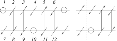
FIG. 1.: Regularly-depleted two-leg spin ladder system with $m=6$. The number assigned to each site is used in the spin-wave analysis in section IV.A.

Although our model seems rather special, it is to be noted that the model contains an essential property expected generally for the depleted models[12]: the gapless states are essentially formed by the coherent motion of unpaired spins generated by the depletion,[9] though an unpaired spin may be a rather complicated object in general. For example, in the case where the period of the depletion is large (dilute limit of impurities), our model reproduces the known results for the system with a few non-magnetic impurities. But also for the high density limit, we can discuss what is essential for the formation of a gapless state in the depleted systems. Moreover, since we can give a rigorous statement for the model, it may serve as a key model by which we can check whether an approximate treatment works well or not when we study wider class of depleted ladder systems. In fact, we will treat a slightly different model in the next section, for which the exact results obtained in this section provide a guideline for analyzing the results correctly.

B The Lieb, Schultz and Mattis Theorem

By using the Lieb, Schultz and Mattis (LSM) theorem [14], we now prove that the depleted model (3) indeed has an excited state of $O(1/N)$. The LSM theorem is elementary, but provides quite powerful tool to demonstrate that a given system is gapless or has degenerate ground states. This theorem can be applied not only to half-odd integer spin models[14, 15] but also to the spin ladder systems, which suggests that odd-leg ladder models are expected to have massless excitations, while it is not applicable to even-leg ladder models, indicating the presences of an excitation gap. The relation between the LSM scheme and the massive RVB states was discussed previously in detail in literature (see for example Ref.14 and references therein).

We now wish to apply this theorem to the depleted model (3). The theorem uses two properties. One is the symmetry of the model based on the translation combined with reflection. The other is the response of the ground state energy to twisted boundary conditions, or equivalently to external gauge fields. This plays an important role for studying low-energy properties in quantum many-body systems. In particular, such effects appear in quite different ways for massless and massive systems. For example, for massless systems, the ground state energy increases as a function of the twist angle of $O(1/N)$, where $N$ is the size of the system, so that the ground state changes into one of the excited states when we follow the spectral flow of the ground state up to the twist angle $\Phi=2\pi$[17, 18]. On the other hand, for massive systems, there is a gap above the ground state of $O(1)$, and hence we cannot reach the excited states by twisting the ground state. In this way, we can use twisted boundary conditions to find a gapless excitation.

We now turn to the question whether we can find such an excitation of $O(1/N)$ in the present model. To this end, let us introduce the operator $T_{m/2}$ for $m/2$-lattice translation and the reflection operator $R$,

$$T_{m/2}\mbox{\boldmath$S$}_{j}^{(i)}T_{m/2}^{-1}=\mbox{\boldmath$S$}_{j+m/2}^{(i)},$$ (5)

$$R\mbox{\boldmath$S$}_{j}^{(1,2)}R^{-1}=\mbox{\boldmath$S$}_{j}^{(2,1)}.$$ (6)

Let $O$ be the product operator $O=RT_{m/2}$. The total Hamiltonian is invariant under the operation of $O$ since $OH^{(1,2)}O^{-1}=H^{(2,1)}$ and $OH_{\rm coup}O^{-1}=H_{\rm coup}$. On the other hand, for a finite size system the ground state is non degenerate within the subspace of fixed $S^{z}_{tot}$ ($=0$), so that we can write $O|\Psi_{0}\rangle=e^{i\alpha}|\Psi_{0}\rangle$.

Now we introduce the twist operator, which plays the central role in the LSM theorem,

$$U^{(i)}=\exp\left[\frac{2\pi i}{N}\sum_{j=0}^{N-1}(1-\theta_{j}^{(i)})jS_{j}^{(i)z}\right].$$ (7)

This operator transforms under $O$ such that

$$OU^{(1)}O^{-1}= U^{(2)}\exp\left(-\frac{m\pi i}{N}S^{(2)z}\right)$$ (9)

$$\times\exp\left[2\pi i\sum_{j=0}^{m/2-1}(1-\theta_{j}^{(2)})S_{j}^{(2)z}\right],$$

$$OU^{(2)}O^{-1}= U^{(1)}\exp\left(-\frac{m\pi i}{N}S^{(1)z}\right),$$ (11)

$$\times\exp\left[2\pi i\sum_{j=0}^{m/2-1}(1-\theta_{j}^{(1)})S_{j}^{(1)z}\right],$$

and therefore $U=U^{(1)}U^{(2)}$ is transformed as

$$OUO^{-1}= U\exp\left(-\frac{m\pi i}{N}S^{z}\right)$$ (13)

$$\times\exp\left[2\pi i\sum_{i=1}^{2}\sum_{j=0}^{m/2-1}(1-\theta_{j}^{(i)})S_{j}^{(i)z}\right]$$

$$= -U.$$ (14)

The second line comes from the facts that we are concerned with the total spin $S^{z}=0$ sector and that in the last exponential there are $m-1$ (odd) spins inside of the dashed box in Fig.1, each of which gives the factor $-1$. Owing to this property, we can construct an excited state $|\Psi\rangle=U|\Psi_{0}\rangle$ with different “parity”, which is orthogonal to the ground state, $\langle\Psi_{0}|\Psi\rangle=0$.

The remaining task is to calculate the energy increment $\delta E=\langle\Psi|H|\Psi\rangle-\langle\Psi_{0}|H|\Psi_{0}\rangle$. We have

$$\delta E= \sum_{i=1}^{2}\sum_{j=0}^{N-1}(1-\theta_{j}^{(i)})(1-\theta_{j+1}^{(i)})$$ (17)

$$\times\left(\cos\frac{2\pi}{N}-1\right)\langle\Psi_{0}|S_{j}^{(i)+}S_{j}^{(i)-}|\Psi_{0}\rangle$$

$$\leq 2(N-M)\left(1-\cos\frac{2\pi}{N}\right)<2\left(1-\frac{2}{m}\right)\frac{4\pi^{2}}{N}.$$

Namely, the excited state orthogonal to the ground state has the excitation energy of $O(1/N)$. Therefore, we end up with the rigorous statement that our model (3) for regularly depleted ladder systems has either the massless spin excitations or the ground state is degenerate in the thermodynamic limit. In subsequent sections, we will focus our attention to the question whether low-energy excitations of our system are indeed massless, and, if so, which type of spin excitations contributes to this massless mode.

Before concluding this section, we wish to remark the following points. As mentioned above, it is the most crucial point in the LSM theorem whether we can construct a state orthogonal to the ground state by the use of the twist operator. In the present system, an unpaired spin in the dashed box in Fig.1 gives the factor $-1$. In the ordinary two-leg ladder systems without depletion, we have always an even number of spins inside the dashed box (however, in this case translation by one site is sufficient to consider, which still gives the factor $(-1)^{2}=1$). Therefore, we can explicitly see that a drastic change in the ground state directly reflects how the phase coherence of the wave function is changed by the depletion.

Some aspects of the ground state can be discussed by applying Marshall’s theorem to our model.[19, 20] The ground state has the spin quantum number $S=0~{}(M)$ for $m=4~{}(2)$ mod 4, so that the ground state of our model is either a spin singlet or partially ferromagnetic. Therefore, in the partially ferromagnetic case, the ground state itself is degenerate, since the state under consideration ($S^{z}=0$ state) is, of course, a member of the spin $S=M$ multiplet. As mentioned in the introduction, this can be easily understood by noticing that the effective interaction between the unpaired spins is ferromagnetic (antiferromagnetic) if the depleted sites are on the same (different) sublattice(s).[10]

III Weak-coupling approach to Hubbard ladder

In the previous section, we have proved that our model for the regularly depleted ladder systems is characterized by massless spin excitations or degenerate ground states with a gap. In order to determine which possibility is actually realized and to study, if possible, the nature of elementary excitations in more detail, we wish to introduce a low-energy effective theory in the continuum limit and study its low-energy properties by using the renormalization group (RG) method. One immediately notices, however, that it is not straightforward to study the effect of the periodic depletion in an ordinary bosonization approach. For example, we cannot take a conventional way in which each chain is first bosonized and the inter-chain coupling is then taken into account via the RG procedure, because a bare single chain would be divided into many disconnected pieces by the depleted sites. To avoid this difficulty, it is desirable to find a way to include the effect of the periodic depletion after bosonization. Based on these observations we introduce a Hubbard-type ladder model in which the effect of the depletion is incorporated in terms of the on-site interaction. We then investigate its low-energy properties by the one-loop RG method. We will use the notations similar to those of Balants and Fisher[21], who studied the ordinary Hubbard type ladder systems without depletion.

A Model

The Hamiltonian we consider is the two-leg ladder of correlated electrons,

$$H= \sum_{i=1}^{2}(H_{\rm hop}^{(i)}+H_{\rm int}^{(i)})+H_{\rm coup},$$ (21)

$$H_{\rm hop}^{(i)}=-t\sum_{j=0}^{N-1}\sum_{\sigma}\left(c_{j\sigma}^{(i)\dagger}c_{j+1\sigma}^{(i)}+h.c.\right),$$

$$H_{\rm int}^{(i)}=\sum_{j=0}^{N-1}(U+U^{\prime}\theta_{j}^{(i)})n_{j\uparrow}^{(i)}n_{j\downarrow}^{(i)},$$

$$H_{\rm coup}=J\sum_{j=0}^{N-1}(1-\theta_{j}^{(1)})(1-\theta_{j}^{(2)})\mbox{\boldmath$S$}_{j}^{(1)}\cdot\mbox{\boldmath$S$}_{j}^{(2)},$$

where we have introduced two types of the Hubbard interactions $U>0$ and $U+U^{\prime}<0$. The interaction $U$ is introduced to produce Heisenberg spins on the lattice sites for large $U$. On the other hand, the attractive interaction $U^{\prime}$ is introduced to effectively represent the depleted spins. Namely, in the $U+U^{\prime}\rightarrow-\infty$ limit, electrons on $j=0~{}(m/2)$ mod $m$ sites for chain-1 (-2) form bound states, i.e. onsite spin singlets, and hence the spin degrees of freedom are effectively frozen out on these sites, as illustrated in Fig.2. In order to correctly reproduce the depleted ladder systems, the number of electrons should be $2(N+M)$, and then the corresponding Fermi momentum is

$$k_{F}=\frac{\pi}{2a_{0}}\left(1+\frac{1}{m}\right),$$ (22)

where $a_{0}$ is the lattice constant.

FIG. 2.: Schematic illustration of the two-leg Hubbard ladder in the strong-coupling limit $U^{\prime}\rightarrow-\infty$

We now investigate low-energy properties of this model with the RG method. Passing to the continuum limit, the fermion operators become

$$c_{j\sigma}^{(i)}/\sqrt{a_{0}}\rightarrow e^{-ik_{F}x}\psi_{iL\sigma}(x)+e^{ik_{F}x}\psi_{iR\sigma}(x)$$ (23)

with $aj\rightarrow x$, and the hopping Hamiltonian is reduced to

$$H_{\rm hop}^{(i)}=v_{F}\int dx\Bigg{[} \frac{\pi}{8}(J_{iL}^{0}J_{iL}^{0}+J_{iR}^{0}J_{iR}^{0})$$ (25)

$$+\frac{2\pi}{3}(J_{iL}^{a}J_{iL}^{a}+J_{iR}^{a}J_{iR}^{a})\Bigg{]}$$

where $v_{F}=2ta_{0}\cos(\pi/2m)$. Here and in what follows, operator products should be normal-ordered, though we do not explicitly indicate this. $J_{iL(R)}^{\mu}$ is the left (right) component of the U(1) and SU(2) currents defined by

$$J_{iL(R)}^{\mu}(x)=\psi_{iL(R)\alpha}^{\dagger}\frac{\sigma^{\mu}_{\alpha\beta}}{2}\psi_{iL(R)\beta}(x),$$ (26)

where $\sigma^{0}$ is the unit matrix: The component $\mu=0$ is the usual U(1) current divided by 2, and those with $a=\mu=1,2,3$ are the SU(2) currents, respectively. Next we bosonize the Hubbard interaction in this approximation. In the following we neglect the oscillating terms which are incommensurate with the Fermi momentum and $\theta_{j}^{(i)}$, as they may disappear after the integration. According to calculations briefly summarized in Appendix A, the intra-chain interaction leads to the following Hamiltonian density,

$$-{\cal H}_{\rm int}= \widetilde{g}_{\rho}J_{iL}^{0}J_{iR}^{0}+\widetilde{g}_{x\rho}(J_{1L}^{0}J_{2R}^{0}+J_{2L}^{0}J_{1R}^{0})$$ (29)

$$+\widetilde{g}_{u}(-)^{i-1}(M_{iL}M_{iR}^{\dagger}+M_{iL}^{\dagger}M_{iR})$$

$$+\widetilde{g}_{\sigma}J_{iL}^{a}J_{iR}^{a},$$

where

$$M_{iL(R)}(x)=\psi_{iL(R)\downarrow}\psi_{iL(R)\uparrow},$$ (30)

and we have dropped the chiral interactions because they merely renormalize the Fermi velocities. Here, repeated indices $i$ and $a$ are summed over. Note that the Umklapp interaction appears though the density of the system under consideration is more than half-filling. This is due to the existence of $\theta_{j}$ in eq.(21), which fixes $U^{\prime}$ on regularly placed lattice sites. We can also take the continuum limit of the inter-chain coupling

$$-{\cal H}_{\rm coup}= \widetilde{g}_{x\sigma}(J_{1L}^{a}J_{2R}^{a}+J_{2L}^{a}J_{1L}^{a})+\widetilde{g}_{t\sigma}(L_{L}^{a}L_{R}^{a\dagger}+L_{L}^{a\dagger}L_{R}^{a})$$ (32)

$$+\widetilde{g}_{t\rho}(L_{L}^{0}L_{R}^{0\dagger}+L_{L}^{0\dagger}L_{R}^{0})$$

where $L_{L(R)}$ is the staggered components of the spin operator

$$L_{L(R)}^{\mu}=\psi_{1L(R)\alpha}^{\dagger}\frac{\sigma^{\mu}_{\alpha\beta}}{2}\psi_{2L(R)\beta}$$ (33)

The initial values of these coupling constants are given by the Hubbard and inter-chain interactions, as summarized in Table I, where we have defined $\widetilde{U}^{\prime}=U^{\prime}/m,\widetilde{U}=U+\widetilde{U}^{\prime}$ and $\widetilde{J}=J(1-2/m)$.

$\widetilde{g}_{\rho}$	$\widetilde{g}_{x\rho}$	$\widetilde{g}_{u}$	$\widetilde{g}_{\sigma}$	$\widetilde{g}_{x\sigma}$	$\widetilde{g}_{t\sigma}$	$\widetilde{g}_{t\rho}$
$-2\widetilde{U}a_{0}$	0	$-\widetilde{U}^{\prime}a_{0}$	$2\widetilde{U}a_{0}$	$-\widetilde{J}a_{0}$	$-\frac{1}{2}\widetilde{J}a_{0}$	$\frac{3}{2}\widetilde{J}a_{0}$

TABLE I.: Coupling constants

The bosonized forms of the interactions are also listed in Appendix C.

B RG Equations and Flows

We now derive the RG equations for the above coupling constants in one-loop order. Using the operator product expansions and resultant RG equations given in Appendix B, we end up with the following set of scaling equations,

$$\frac{dg_{\rho}}{dl}=-4g_{u}^{2}-\frac{1}{4}(g_{t\rho}^{2}+3g_{t\sigma}^{2}),$$ (34)

$$\frac{dg_{x\rho}}{dl}=\frac{1}{4}(g_{t\rho}^{2}+3g_{t\sigma}^{2}),$$ (35)

$$\frac{dg_{u}}{dl}=-g_{\rho}g_{u},$$ (36)

$$\frac{dg_{\sigma}}{dl}=-g_{\sigma}^{2}-\frac{1}{2}(g_{t\sigma}+g_{t\rho})g_{t\sigma},$$ (37)

$$\frac{dg_{x\sigma}}{dl}=-g_{x\sigma}^{2}-\frac{1}{2}(g_{t\sigma}-g_{t\rho})g_{t\sigma},$$ (38)

$$\frac{dg_{t\sigma}}{dl}=-\left[\frac{1}{2}(g_{\rho}-g_{x\rho})+(g_{\sigma}+g_{x\sigma})\right]g_{t\sigma}$$ (39)

$$\qquad\qquad\qquad-\frac{1}{2}(g_{\sigma}-g_{x\sigma})g_{t\rho},$$ (40)

$$\frac{dg_{t\rho}}{dl}=-\frac{1}{2}(g_{\rho}-g_{x\rho})g_{t\rho}-\frac{3}{2}(g_{\sigma}-g_{x\sigma})g_{t\sigma}$$ (41)

with $l=\ln L$, where $g_{k}=\widetilde{g}_{k}/2\pi v_{F}$.

We have numerically integrated the above set of equations to obtain the RG flows. Typical examples of the RG flows are shown in Figs.3 and 4.

FIG. 3.: RG flows for (a) $g_{\rho}$, (b) $g_{u}$, (c) $g_{t\sigma}$ and (d) $g_{t\rho}$: Plotted values are multiplied by the factor 10. $g_{x\rho}\sim 0$ in this figure. The parameters used are $U=1,U^{\prime}=-20,j=0.01$ and $m=50$.

FIG. 4.: RG flows for (a) $g_{\sigma}$ and (b) $g_{x\sigma}$: Plotted values are multiplied by the factor 400. The parameters used are the same as those in Fig.3.

We note that a characteristic scale $l_{c}$ exists, at which all renormalized couplings except for $g_{x\rho}$ exhibit divergence properties, though those in Fig.4 look convergent at a first glance. We will see below that this divergence is mainly driven by the charge sector, so that $l_{c}$ may be identified with the scale at which the mass gap is generated for the charge sector. Accordingly, couplings for other spin modes are strongly affected. In what follows, we analyze characteristic properties of RG flows around $l_{c}$ analytically. Note first that the key parameter in our approach is $U^{\prime}$, which would make singlet bound pairs on particular sites, freezing out the spin degrees of freedom. Now we fix the other parameters, e.g. $U=1,m=50,J=0.01$. In this case, the Umklapp interaction turns out to be relevant in the range $U^{\prime}_{c}<U^{\prime}<0$ ( $U^{\prime}_{c}\sim-40$ for this particular choice of interactions. We will explain the meaning of $U_{c}^{\prime}$ below). In this range, $g_{\rho}$ is most relevant and we can neglect $g_{t\sigma}$ and $g_{t\rho}$ eqs.(34)$\sim$(36), resulting in

$$\frac{dg_{\rho}}{dl} \sim -4g_{u}^{2},$$ (42)

$$\frac{dg_{u}}{dl} \sim -g_{\rho}g_{u},$$ (43)

near the divergent point. This is a familiar U(1) scaling equation, from which we obtain $g_{\rho}\sim-1/(l_{c}-l)$. This expression near the divergent point is confirmed by the numerical integration of the RG equations. This result means that the charge gap is generated by the Coulomb interactions $U$ and $U^{\prime}$.

What happens for the spin sector in this case ? Note that the next relevant interactions are the inter-chain staggered interactions $g_{t\sigma}$ and $g_{t\rho}$ for the spin sector, since they act as composite of spin and charge degrees of freedom, the dimension of which is unity if we replace the massive charge degree of freedom by its mean value, as can be seen in Table.II. Neglecting small terms, we thus obtain

$$\frac{dg_{t\sigma}}{dl} \sim -\frac{1}{2}g_{\rho}g_{t\sigma},$$ (44)

$$\frac{dg_{t\rho}}{dl} \sim -\frac{1}{2}g_{\rho}g_{t\rho}.$$ (45)

Using the above-obtained $g_{\rho}$ for the charge sector, we have the RG flows

$$g_{t\sigma} \sim \frac{g_{t\sigma 0}}{(l_{c}-l)^{1/2}},$$ (46)

$$g_{t\rho} \sim \frac{g_{t\rho 0}}{(l_{c}-l)^{1/2}},$$ (47)

near the divergent point. Therefore, it is seen that the spin modes scale to the strong coupling fixed-point and the spin gap is still open. This may not be plausible for the depleted spin ladders, according to the rigorous theorem obtained in the previous section. This is because the effect of the depletion is not fully taken into account in the present one-loop RG method.[22] It should be noted, however, that the effect of the depletion actually has the tendency to make the spin sector massless. Namely, we can indeed see that the coefficients $g_{t\sigma 0}$ and $g_{t\rho 0}$ quickly decrease with increasing $|U^{\prime}|$. [23] In fact from the numerical integration of the RG equations, we estimate them as

$$g_{t\sigma 0},g_{t\rho 0}\sim\frac{\mbox{const.}}{|U^{\prime}|^{\alpha}},$$ (48)

with $\alpha\sim 1$ (See Fig.5).

FIG. 5.: (a) $-g_{t\sigma 0}\times 10^{3}$ and (b) $g_{t\rho 0}\times 2\cdot 10^{2}$ as functions of negative $U^{\prime}$.

Therefore, although the spin gap still exists for finite $U^{\prime}$, we can expect, by smooth extrapolation to $U^{\prime}\rightarrow-\infty$, that the divergence in the above RG flows may be suppressed, leading to the massless spin modes.

We should mention here that the above treatment would fail at some negative critical value $U^{\prime}=U^{\prime}_{c}$ if we only increase $|U^{\prime}|$ by keeping $U$ fixed. Namely, for $|U^{\prime}|>U^{\prime}_{c}$, the charge mode becomes massless, and then we cannot use the model as a weak-coupling analog of the depleted lattice. This pathological result may come from the fact that the extremely strong attractive $U^{\prime}$ may overwhelm the repulsive $U$ completely, resulting in the spin bound states similarly to the attractive Hubbard model and hence making the charge mode massless. So, it may be necessary to take a strong-coupling limit by appropriately tuning the ratio of $U$ and $U^{\prime}$ in the present model with attractive $U^{\prime}$.

C Discussions

Within the above analysis for the effective weak coupling model, it turns out that the model is still massive for any finite coupling, though the tendency to gapless excitations is seen as the singlet bound state becomes strong. This may suggest that it is not straightforward to incorporate the effects of depletion in a conventional continuum limit. In this sense, we should say that our analysis in this section is not satisfactory to describe massless excitations in the depleted spin model. In this connection, we would like to note here that the present RG analysis is based on the effective weak-coupling “electron” model because we believe that this electron model belongs to the same universality class of the original spin model. In fact we have numerically solved the RG equations not only for the spin sector but also for the charge sector, and found that all the trajectories flow to the strong coupling fixed points. Furthermore, as an extension, one could examine whether the above situation is improved if we solve the RG equations only for spin sectors by discarding the charge degrees of freedom, which should be a more accurate approximation for the original spin model. Unfortunately, even if we concentrate on the RG equations for the spin sector, we still encounter the problem that the spin sector is massive since the dimension of the inter-chain couplings reduce to 1, as can be seen from Table II. In this sense, a conventional weak-coupling bosonization approach, in which two chains are assumed to be weakly coupled with each other, does probably not allow a straightforward description of the low-energy properties of the depleted model. We thus have to find or develop a more effective way to incorporate the effect of depletion correctly. This problem will be discussed in the following section.

IV Non-linear sigma model approach

In the previous section, we have seen that it is not straightforward to incorporate the effect of depletion in an ordinary weak-coupling approach. In particular, it is quite difficult in this weak-coupling model to figure out which kind of spin excitations would actually become massless. To clarify this point, and also to confirm that the massless modes are actually realized, we would like to consider a different field theoretical approach by using non-linear sigma model techniques.[24, 25, 26, 11]

Let us reconsider here the essential ingredients important for low energy excitations in our model. When applying the LSM theorem in sec.II, we have seen that the presence of unpaired spins associated with vacant sites play a crucial role. All other spins are essentially bound into local singlet pairs and cannot contribute to the very low energy spectrum. The vacant sites break the uniformity of the system by introducing these unpaired spin degrees of freedom and by the local polarization of a staggered moment in their vicinity. A short-ranged effective interaction among the unpaired spins is mediated through polarization of the remaining spins, which is (anti-)ferromagnetic for $m=2~{}(4)$ mod 4. These interactions are weak and are assumed to introduce a gapless spectrum. In a weak coupling approach in the previous section, we have started with ordinary boson fields by simply applying the conventional bosonization schemes to each chain, and have not explicitly taken into account the above properties in the beginning. Therefore, in order to describe the massless mode better, we need a rather complicated combination of these boson fields by incorporating higher-order interactions. This may be a reason why it was difficult in the weak coupling model to explicitly construct the massless spin excitations.

Based on these observations, we would like to consider below a complementary approach which allows us to describe the formation of massless excitations more easily. We will concentrate on the regime of comparatively small $m$ where the background of the staggered magnetization plays an important role. We first perform a spin-wave analysis of the depleted model to clarify the nature of spin excitations. We then convert the lowest spin mode to the non-linear sigma model, finding that the massless excitations are indeed generated for the depleted model.

A Spin-Wave Analysis

We consider now a regularly depleted spin ladder with rather small $m$. Then the polarization cloud of staggered magnetization around each vacancy have a strong overlap with each other. Assuming coherent, though slightly inhomogeneous staggered magnetization throughout the whole ladder we may use the Holstein-Primakoff mapping. Because after regular depletion (period $m$) the unit cell of the ladder is large we represent the spin operators by $2m$ kind of bosons $a_{l}^{(i)}$ with $i=1,2$ and $l=0,1,\cdots m-1$ (We here include the depleted sites $i=1,~{}l=0$ and $i=2,~{}l=m/2$ for simplicity. But their sector easily decouples, which has always zero-energy),

$$S^{(i)z}_{mj+l}=\pm\left(\frac{1}{2}-n_{l}^{(i)}(mj+l)\right),$$ (49)

$$S^{(i)+}_{mj+l}=\left\{\begin{array}[]{c}\sqrt{1-n_{l}^{(i)}(mj+l)}a_{l}^{(i)}(mj+l)\\ a_{l}^{(i)\dagger}(mj+l)\sqrt{1-n_{l}^{(i)}(mj+l)}\end{array}\right.\quad$$ (52)

where $n_{l}$ is the number operator. In (4.2) we take the upper (lower) relation for $i+l=$ odd (even). In the momentum representation,

$$a_{l}^{(i)}(mj+l)=\frac{1}{\sqrt{M}}\sum_{k=0}^{M-1}\exp\left[\frac{2\pi i}{N}(mj+l)k\right]a_{l}^{(i)}(k),$$ (53)

the Hamiltonian becomes, up to quadratic order of the boson operators,

$$H=\sum_{k}\sum_{i,j=1}^{2m}\left(a_{i}^{\dagger}h_{ij}a_{j}+a_{i}h_{ij}a_{j}^{\dagger}+a_{i}^{\dagger}\Delta_{ij}a_{j}^{\dagger}+a_{i}\bar{\Delta}_{ij}a_{j}\right)$$ (54)

where we have omitted some trivial constant terms. We have used a simplified notation (See Fig.1 for this numbering), $a_{0}^{(1)}(k)=a_{1}$, $\cdots,a_{m-1}^{(1)}(-k)=a_{m}$, $a_{0}^{(2)}(-k)=a_{m+1}$, $\cdots$, $\cdots$, $a_{m-1}^{(2)}(k)=a_{2m}$, and the $2m\times 2m$ matrices $h$ and $\Delta$ are given in Appendix D. By the Bogoliubov transformation

$$a_{i}=\sum_{j=1}^{2m}\left(U_{ij}b_{j}+\bar{V}_{ij}b_{j}^{\dagger}\right),$$ (55)

which should satisfy the relations

$$UV^{\dagger}-\bar{V}U=0,\quad UU^{\dagger}-\bar{V}V^{T}={\boldmath 1},$$ (56)

we can reach the diagonal form of the Hamiltonian, up to constant terms,

$$H=\sum_{j=1}^{2m}\omega_{j}b_{j}^{\dagger}b_{j}+\hbox{const.},$$ (57)

In Figs.6,7, we show the dispersion $\omega_{i}$ as a function of $k$, in which we omitted the zero-energy modes associated with depleted spins. We can observe that several bands appear because of the periodic depletion. It is remarkable that within this approach the difference between the cases $m=2$ and $m=4$ (mod 4) is reproduced clearly.

FIG. 6.: Dispersion of $m=6$ system with $J=1$ as functions of $k$ with $N=600$. In the usual notation, $k=100$ point corresponds to the momentum $2\pi i\times 100/600=\pi/3$. See eq.(D6)

FIG. 7.: Dispersion of $m=8$ system with $j=1$ as functions of $k$ with $N=800$. In the usual notation, $k=100$ point corresponds to the momentum $2\pi i\times 100/800=\pi/4$.

As discussed in section II, the ground state of the former case is ferromagnetic (partially spin polarized), which is reflected in the quadratic dispersion of the lowest band for the small momenta (Fig.6). In contrast the latter behaves quite differently, displaying a linear low-energy spectrum. Therefore, the lowest band is indeed due to the interaction between unpaired spins, as discussed at the beginning of this section. Though the lowest spin mode does not have an excitation gap in both cases, one cannot naively conclude a gapless spectrum for the system, because higher-order quantum corrections play an important role to determine whether or not the system is indeed gapless. This problem is investigated in the subsection B.

We would like to mention here that although our approach is valid for the case of small $m$, the qualitative properties of the low-energy spin excitation spectrum are the same for large $m$. In this case, however, a quantitative description would have to include the effects of the coupling among elementary excitations beyond (4.4) and (4.7). It is not our aim to address this problem here.

B Mapping to the Non-Linear Sigma Model

Based on the above spin-wave analysis, we would like to now consider the lowest band due to the unpaired spins and to discuss the role of quantum effects by employing sigma model techniques. The results in the previous subsection suggest that the system with $m=4$ (mod 4) can be mapped to the non-linear sigma model, as is usually the case for uniform spin chains as well as uniform spin-ladder systems. We restrict ourselves to such cases in this section.

We use here the coherent state path-integral method.[27] The partition function $Z={\rm tr}\exp(-\beta H)$ can be represented by $Z=\int\prod_{i,j}{\cal D}[\mu(\mbox{\boldmath$N$}^{(i)}(j))]\exp(-S)$, where the unit vector $\mbox{\boldmath$N$}^{(i)}(j)$ specifies the coherent state of the spin at the $j$th site of the $i$th chain such that $\langle\mbox{\boldmath$N$}^{(i)}(j)|\mbox{\boldmath$S$}_{j}^{(i)}|\mbox{\boldmath$N$}^{(i)}(j)\rangle=s\mbox{\boldmath$N$}^{(i)}(j)$ with $s=1/2$, and $\mu(\mbox{\boldmath$N$})$ is the invariant measure $\int d\mu(\mbox{\boldmath$N$})|\mbox{\boldmath$N$}\rangle\langle\mbox{\boldmath$N$}|=1$. The Euclidean action $S$ is

$$S=S_{B}+S_{\|}+S_{\bot},$$ (58)

where

$$S_{B}=-is\sum_{i=1}^{2}\sum_{j=0}^{N-1}(1-\theta_{j}^{(i)})\omega[\mbox{\boldmath$N$}^{(i)}(j)],$$ (59)

$$S_{\|}=s^{2}\int_{0}^{\beta}\!\!d\tau\sum_{i=1}^{2}\sum_{j=0}^{N-1}(1-\theta_{j}^{(i)})(1-\theta_{j+1}^{(i)})$$ (60)

$$\qquad\qquad\qquad\qquad\qquad\times\mbox{\boldmath$N$}^{(i)}(j)\cdot\mbox{\boldmath$N$}^{(i)}(j+1),$$ (61)

$$S_{\bot}=Js^{2}\int_{0}^{\beta}\!\!d\tau\sum_{j=0}^{N-1}(1-\theta_{j}^{(1)})(1-\theta_{j}^{(2)})$$ (62)

$$\qquad\qquad\qquad\qquad\qquad\times\mbox{\boldmath$N$}^{(1)}(j)\cdot\mbox{\boldmath$N$}^{(2)}(j).$$ (63)

Here $\omega[\mbox{\boldmath$N$}]$ is the Berry phase defined by

$$\omega[\mbox{\boldmath$N$}]=\int_{0}^{\beta}\!\!d\tau\!\!\int_{0}^{1}\!\!du\mbox{\boldmath$N$}\cdot(\partial_{\tau}\mbox{\boldmath$N$}\times\partial_{u}\mbox{\boldmath$N$}).$$ (64)

After staggering the configuration

$$\mbox{\boldmath$N$}^{(i)}(j)=(-)^{i+j+1}\mbox{\boldmath$n$}^{(i)}(j),$$ (65)

we suppose

$$\mbox{\boldmath$n$}^{(i)}(j)=\mbox{\boldmath$m$}(j)+(-)^{i+j+1}a_{0}\mbox{\boldmath$l$}(j).$$ (66)

In what follows, we assume the fields $m$ and $l$ are sufficiently smooth functions. If we want to describe not only the lowest band but also the massive bands, we must include several kinds of fields. However, we concentrate on the lowest one only. We expect that the above (non-trivial) assumption are sufficient for this description.

Let us now derive the continuum limit of the action. First we consider the Berry phase term and divide it into two contributions,

$$S_{B} = -is\sum_{i=1}^{2}\sum_{j=0}^{N-1}(-)^{i+j+1}\omega[\mbox{\boldmath$n$}^{(i)}(j)]$$ (68)

$$+is\sum_{i=1}^{2}\sum_{j=0}^{N-1}(-)^{i+j+1}\theta_{j}^{(i)}\omega[\mbox{\boldmath$n$}^{(i)}(j)].$$

Taking now the continuum limit in each chain in eq.(68), the topological terms cancel out due to the factor $(-)^{i}$, and we find

$$(\ref{Ber1})=2is\int\!\!d^{2}x\mbox{\boldmath$l$}\cdot(\mbox{\boldmath$m$}\times\partial_{2}\mbox{\boldmath$m$}),$$ (69)

where $x_{1}=x~{}(=a_{0}j)$ and $x_{2}=\tau$. Then the contribution from eq.(68) is evaluated

$$(\ref{Ber2}) = is\sum_{j=1}^{M-1}\left\{\omega[\mbox{\boldmath$n$}^{(1)}(mj)]-\omega[\mbox{\boldmath$n$}^{(2)}(mj+m/2)]\right\}$$ (70)

$$\sim is\sum_{j=1}^{M-1}\int\!\!d\tau(-)\delta\mbox{\boldmath$n$}^{(1)}(mj)$$ (72)

$$\qquad\qquad\cdot\left[\mbox{\boldmath$n$}^{(1)}(mj)\times\partial_{\tau}\mbox{\boldmath$n$}^{(1)}(mj)\right],$$

where $\delta\mbox{\boldmath$n$}^{(1)}(mj)\equiv\mbox{\boldmath$n$}^{(1)}(mj)-\mbox{\boldmath$n$}^{(2)}(mj+\frac{m}{2})\sim-\frac{m}{2}a_{0}\partial_{x}\mbox{\boldmath$m$}(mj)+2a_{0}\mbox{\boldmath$l$}(mj)+O(a_{0}^{2})$. We have assumed that the short-range AF order is strong enough to justify our continuum limit. As noted above in this subsection, we here concentrate on the case $m=4$ (mod 4), because the above equation is valid only for $m/2=$ even. Substituting this relation, we have

$$(\ref{Ber2})= -\frac{is}{2}\int\!\!d^{2}x\mbox{\boldmath$m$}\cdot(\partial_{1}\mbox{\boldmath$m$}\times\partial_{2}\mbox{\boldmath$m$})$$ (74)

$$-\frac{2is}{m}\int\!\!d^{2}x\mbox{\boldmath$l$}\cdot(\mbox{\boldmath$m$}\times\partial_{2}\mbox{\boldmath$m$}).$$

Next, we evaluate the intra-chain interaction. For example, the contribution from chain 1 is

$$S_{\|}^{(1)} = \frac{s^{2}}{2}\int\!\!d\tau\sum_{j=0}^{M-1}\sum_{l=1}^{m-2}\left[\mbox{\boldmath$n$}^{(1)}(mj+l)-\mbox{\boldmath$n$}^{(1)}(mj+l+1)\right]^{2}$$ (75)

$$\sim \frac{a_{0}s^{2}}{2}\sum_{l=1}^{m-2}\int\!\!\frac{dx}{m}\int\!\!d\tau\left[(\partial_{x}\mbox{\boldmath$m$})^{2}-4(-)^{l}\partial_{x}\mbox{\boldmath$m$}\cdot\mbox{\boldmath$l$}+4\mbox{\boldmath$l$}^{2}\right]$$ (76)

$$= \frac{a_{0}s^{2}}{2}\frac{m-2}{m}\int\!\!d^{2}x\left[(\partial_{x}\mbox{\boldmath$m$})^{2}+4\mbox{\boldmath$l$}^{2}\right].$$ (77)

This type of approximation may be justified for rather small $m$ where we can assume that the region between the vacant sites is clearly dominated by the staggered spin polarization. Then all the intermediate spins vary very slowly and essentially in phase with each other. The contribution from chain 2 is exactly the same, and we find

$$S_{\|}=as_{0}^{2}\left(1-\frac{2}{m}\right)\int\!\!d^{2}x\left[(\partial_{x}\mbox{\boldmath$m$})^{2}+4\mbox{\boldmath$l$}^{2}\right].$$ (78)

Inter-chain interaction is similarly evaluated

$$S_{\bot}=2Ja_{0}s^{2}\left(1-\frac{2}{m}\right)\int\!\!d^{2}x\mbox{\boldmath$l$}^{2}.$$ (79)

Collecting terms thus obtained and integrating the field $l$ out, we have $S=\int d^{2}x{\cal L}$, where

$${\cal L}= \frac{1}{2g}\left[v(\partial_{1}\mbox{\boldmath$m$})^{2}+\frac{1}{v}(\partial_{2}\mbox{\boldmath$m$})^{2}\right]$$ (81)

$$\qquad-\frac{\theta}{8\pi}\epsilon_{\mu\nu}\mbox{\boldmath$m$}\cdot(\partial_{\mu}\mbox{\boldmath$m$}\times\partial_{\nu}\mbox{\boldmath$m$}),$$

where

$$\theta=2\pi is=\pi i,$$ (82)

$$g=\frac{m}{s(m-1)}\sqrt{1+r/2},$$ (83)

$$v=2Ja_{0}s\frac{m-2}{m-1}\sqrt{1+r/2},$$ (84)

with $r=1/J~{}(=J_{\|}/J_{\bot})$.

It should be noted here that the topological term in the above action appears with the coefficient $\pi i$, which suggests that the present system should be massless, as we expected. Therefore, combining this result with the analyses in secs. II and III, we end up with the conclusion that the present depleted system with spin singlet ground state should have massless spin excitations, belonging to the same universality class as the uniform $s=1/2$ Heisenberg chain.

Before concluding this section, a brief comment on the case of larger $m$ is in order. As we mentioned, our present approach is valid for the case of rather small $m$. If we naively set $m\rightarrow\infty$, bulk quantities such as $g$ and $v$ in eq.(84) reduce to the formula derived by Dell’Aringa et. al.[26] for the uniform non-depleted spin ladders, while the coefficient $\theta$ remains $\theta=\pi i$. This result seems somewhat paradoxical at first sight. However, one should note that the continuum limit in our approach means $M\equiv N/m\rightarrow\infty$. Therefore, however large $m$ may be, the system always has the periodic array of impurities with finite density (infinite number of impurities in the thermodynamic limit), which may form the massless mode inside of the Haldane gap even for the limit of large $m$. This massless mode should be smoothly extrapolated from the massless mode obtained for the small $m$ case. In this sense, the limit $m\rightarrow\infty$ contains a subtle problem. We think that in the present approximation the topological term $\theta=\pi i$ correctly reflects this massless mode whereas the values of $g$ and $v$ are determined by the host part with the Haldane gap in the large $m$ limit. Therefore, to apply our analysis to the low-energy physics in the large $m$ case consistently, we need to improve systematically the evaluation of the bulk quantities of $g$ and $v$. In fact, we have checked in a preliminary calculation that the estimated values of the above bulk quantities are improved if we include not only the lowest spin mode but also higher modes. From these discussions, we believe that the present conclusion drawn from the above treatment applies also to the case of larger $m$ at least qualitatively, although the approximation becomes worse when $m$ becomes large. To improve our results in the large $m$ case is an open problem to be explored in the future study. Note that in the case of larger $m$, an appropriate scheme to treat low-energy excitations has been considered recently by Nagaosa et al. in the context of a randomly depleted spin ladder [11].

V Summary

We have considered a class of the models for regularly depleted two-leg spin ladder systems, and investigated their low-energy properties. It has been proved rigorously that by the depletion this special class of the models generates a new state which is characterized either by the presence of gapless excitations or a degenerate ground state. To see whether the massless states are really produced by the depletion, we have investigated low-energy properties in terms of two different field theoretical approaches.

We have first proposed a scheme to describe low-energy properties by applying renormalization group methods to an effective weak-coupling model of Hubbard type, in which the effect of the depletion is incorporated in the strong coupling limit of the on-site interaction. This model has been analyzed in a weak coupling approximation based on the one-loop RG method. Although we have seen how the tendency to a massless state is developed when the effect of the depletion becomes strong, it has been found that our model is still massive for any finite couplings. This implies that it is not easy to describe the effect of depletion in a naive continuum limit by a conventional method.

To clarify this point, we studied the depleted spin model by mapping it to the non-linear sigma model. We have found via the spin-wave analysis that the dispersion relation of the lowest spin wave mode has indeed a linear spectrum in the case of the singlet ground state, which allowed us to mapping to the non-linear sigma model with a topological term. It has been shown that the coefficient of this topological term is $\pi i$, which coincides with that of the models which have massless spin excitations such as the spin 1/2 Heisenberg chain. By combining all the analyses in secs.II, III and IV, we thus conclude that the periodic depletion of the present spin ladder systems should produce massless spin excitations.

Finally we note that the drastic change from the spin-gap state to the gapless state observed in the present model reflects that the phase coherence in the wave function is quite sensitive to the depletion. In this sense, the formation of the gapless spin state in our periodic model have the same basic origin as that with random non-magnetic impurities, although the low-temperature thermodynamics of the two is rather different. [10]

A Continuum limit of interactions

In this Appendix, we derive the continuum limit of interactions (29) and (32). First, the continuum limit of the intra-chain interaction is calculated as

$$H_{\rm int}^{(i)}=\int dx \left(Ua+U^{\prime}a\theta_{j}^{(i)}\right)\bigl{(}2J_{iL}^{0}J_{iR}^{0}-2J_{iL}^{a}J_{iR}^{a}$$ (A2)

$$+e^{4ik_{F}x}\psi_{iL\uparrow}^{\dagger}\psi_{iR\uparrow}\psi_{iL\downarrow}^{\dagger}\psi_{iR\downarrow}+{\rm h.c.}\bigr{)}$$

Note here that $\theta_{j}$ defined by eq.(4) can be rewritten as

$$\theta_{j}=\frac{1}{m}\sum_{l=1}^{m}e^{2\pi ilj/m}.$$ (A3)

Therefore, various kinds of terms behave as

$$e^{4ik_{F}x}=e^{2\pi i(1+1/m)j}=\hbox{(ossillating terms)},$$ (A4)

$$\theta_{j}^{(i)}=\frac{1}{m}+\hbox{(ossillating terms)},$$ (A5)

$$\theta_{j}^{(i)}e^{4ik_{F}x}=(-)^{i-1}\frac{1}{m}+\hbox{(ossillating terms)},$$ (A6)

where $i$ in $\theta^{(i)}$ is $i=1,2$. Consequently, if we neglect oscillating terms, we have eq.(29).

Next consider the inter-chain coupling. By using the continuum limit of the spin operator,

$$S_{j}^{(i)a}/a_{0}\rightarrow J_{iL}^{a}+J_{iR}^{a}+\left(e^{2ik_{F}x}N_{i}^{a}+\hbox{ h.c.}\right),$$ (A7)

where

$$N_{i}^{a}=\psi_{iL\alpha}^{\dagger}\frac{\sigma^{a}_{\alpha\beta}}{2}\psi_{iR\beta}.$$ (A8)

the inter-chain coupling terms are calculated as

$$H_{\rm coup}= \int dx\left(1-\theta_{j}^{(1)}\right)\left(1-\theta_{j}^{(2)}\right)$$ (A9)

$$\times \Bigl{[}J_{1L}^{a}J_{2R}^{a}+J_{2L}^{a}J_{1R}^{a}+\left(N_{1}^{a}N_{2}^{a\dagger}+\hbox{h.c.}\right)$$ (A12)

$$~{}+(2k_{F}\hbox{ oscillating terms})$$

$$~{}+(4k_{F}\hbox{ oscillating terms})\Bigr{]}.$$

Note that

$$\left(1-\theta_{j}^{(1)}\right)\left(1-\theta_{j}^{(2)}\right)=1-\frac{2}{m}\sum_{l=1}^{m/2}e^{4\pi ilj/m}.$$ (A13)

Therefore, we have formulae similar to (A6),

$$\left(1-\theta_{j}^{(1)}\right)\left(1-\theta_{j}^{(2)}\right)=1-\frac{2}{m}+\hbox{ (oscillating terms),}$$ (A14)

$$\left(1-\theta_{j}^{(1)}\right)\left(1-\theta_{j}^{(2)}\right)e^{2ik_{F}x}=\hbox{ (oscillating terms)},$$ (A15)

$$\left(1-\theta_{j}^{(1)}\right)\left(1-\theta_{j}^{(2)}\right)e^{4ik_{F}x}=\hbox{ (oscillating terms)}.$$ (A16)

By expressing $N_{1}^{a}N_{2}^{a\dagger}$ by $L$,

$$N_{1}^{a}N_{2}^{a\dagger}+\hbox{h.c.}=\frac{1}{2}(L_{L}^{a}L_{R}^{\dagger a}+\hbox{h.c.})-\frac{3}{2}(L_{L}^{0}L_{R}^{\dagger 0}+\hbox{h.c.}),$$ (A18)

we end up with eq.(32).

B Operator product expansion

The basic operator product expansion (OPE) for Fermi fields is

$$\psi_{iL\alpha}^{\dagger}(z)\psi_{jL\beta}(w)\sim\frac{\delta_{ij}\delta_{\alpha\beta}}{2\pi(z-w)},$$ (B1)

where $z=v_{F}\tau+ix$. Here and in what follows, we neglect regular terms. Operator products should be normal-ordered, though we do not explicitly indicate this. Similar formulae hold for right-moving currents, by replacing $z\rightarrow\bar{z}$. Define $f^{\mu\nu\lambda}$ and $d^{\mu\nu\lambda}$ as $[\sigma^{\mu}/2,\sigma^{\nu}/2]=f^{\mu\nu\lambda}\sigma^{\lambda}/2$ and $\sigma^{\mu}\sigma^{\nu}=d^{\mu\nu\lambda}\sigma^{\lambda}$. Namely, $f^{0\mu\nu}=f^{\mu 0\nu}=f^{\mu\nu 0}=0,~{}f^{abc}=i\epsilon^{abc}$ and $d^{0\mu\nu}=d^{\mu 0\nu}=d^{\mu\nu 0}=\delta^{\mu\nu},~{}d^{abc}=\delta^{ab}\delta^{c0}+i\epsilon^{abc}$. Then we have

$$J_{iL}^{\mu}(z)J_{jL}^{\nu}(w)\sim\delta_{ij}\left[\frac{\delta^{\mu\nu}}{8\pi^{2}(z-w)^{2}}+\frac{f^{\mu\nu\lambda}J_{jL}^{\lambda}(w)}{2\pi(z-w)}\right],$$ (B2)

$$L_{L}^{\mu}(z)L_{L}^{\nu\dagger}(w)\sim\frac{\delta^{\mu\nu}}{8\pi^{2}(z-w)^{2}}$$ (B3)

$$\qquad\qquad\qquad\qquad+\frac{d^{\mu\nu\lambda}J_{1L}^{\lambda}(w)-d^{\nu\mu\lambda}J_{2L}^{\lambda}(w)}{2\pi(z-w)},$$ (B4)

$$L_{L}^{\mu\dagger}(z)L_{L}^{\nu}(w)\sim\quad(1\leftrightarrow 2),$$ (B5)

$$M_{iL}(z)M_{jL}(w)\sim\delta_{ij}\left[\frac{-1}{4\pi^{2}(z-w)^{2}}+\frac{-J_{jL}^{0}}{\pi(z-w)}\right],$$ (B6)

$$J_{iL}^{\mu}(z)L_{L}^{\nu}(w)\sim\frac{(\delta_{i1}d^{\mu\nu\lambda}-\delta_{i2}d^{\nu\mu\lambda})L_{L}^{\lambda}(w)}{4\pi(z-w)},$$ (B7)

$$J_{iL}^{\mu}(z)L_{L}^{\nu\dagger}(w)\sim\quad(1\leftrightarrow 2),$$ (B8)

$$J_{iL}^{\mu}(z)M_{jL}(w)\sim\delta_{ij}\frac{-\delta^{\mu 0}M_{jL}(w)}{2\pi(z-w)}.$$ (B9)

The OPEs among various 4-Fermi interactions in the text follow from the above formulae. Using these OPEs, we can derive the one-loop order RG equation as follows: Suppose

$$H=H_{*}-\sum_{i}\frac{g_{i}}{2\pi v_{F}}\int dxO_{i},$$ (B10)

where the operators $O_{i}$ represent the various 4-Fermi interactions with dimension 2 given above. The RG equations for such perturbations are given by

$$\frac{dg_{k}}{dl}=(2-x_{k})g_{k}+2\pi^{2}\sum_{i,j}C_{ijk}g_{i}g_{j},$$ (B11)

where $x_{k}$ is the dimension of the operator $O_{k}$ and $C_{ijk}$ is the OPE coefficients defined by

$$O_{i}(z)O_{j}(w)\sim\sum_{k}\frac{C_{ijk}}{|z-w|^{2}}O_{k}(w).$$ (B12)

C Bosonization

The Fermi fields are bosonized as

$$\psi_{iL\alpha} = \frac{1}{\sqrt{2\pi a}}e^{-i\sqrt{4\pi}\varphi_{iL\alpha}},$$ (C1)

$$\psi_{iR\alpha} = \frac{1}{\sqrt{2\pi a}}e^{i\sqrt{4\pi}\varphi_{iR\alpha}}.$$ (C2)

Define

$$\varphi_{i\alpha} = \varphi_{iL\alpha}+\varphi_{iR\alpha},$$ (C3)

$$\theta_{i\alpha} = \varphi_{iL\alpha}-\varphi_{iR\alpha},$$ (C4)

and

$$\varphi_{ic}=\frac{1}{\sqrt{2}}(\varphi_{i\uparrow}+\varphi_{i\downarrow}),\quad\theta_{ic}=\frac{1}{\sqrt{2}}(\theta_{i\uparrow}+\theta_{i\downarrow}),$$ (C5)

$$\varphi_{is}=\frac{1}{\sqrt{2}}(\varphi_{i\uparrow}-\varphi_{i\downarrow}),\quad\theta_{is}=\frac{1}{\sqrt{2}}(\theta_{i\uparrow}-\theta_{i\downarrow}).$$ (C6)

For ladder systems, it is convenient to define furthermore the in- and out-of-phase Bose fields,

$$\varphi_{c}^{\pm}=\frac{1}{\sqrt{2}}(\varphi_{1c}\pm\varphi_{2c}),\quad\theta_{c}^{\pm}=\frac{1}{\sqrt{2}}(\theta_{1c}\pm\theta_{2c}),$$ (C7)

$$\varphi_{s}^{\pm}=\frac{1}{\sqrt{2}}(\varphi_{1s}\pm\varphi_{2s}),\quad\theta_{s}^{\pm}=\frac{1}{\sqrt{2}}(\theta_{1s}\pm\theta_{2s}).$$ (C8)

Then, except for the gradient terms, we have the bosonized form of the various interactions in the text, summarized in the Table II.

Coupling constants	Corresponding operators
$g_{u}$	$\frac{1}{\pi^{2}a^{2}}\sin\sqrt{4\pi}\varphi_{c}^{+}\sin\sqrt{4\pi}\varphi_{c}^{-}$
$g_{\sigma}$	$\frac{-1}{2\pi^{2}a^{2}}\cos\sqrt{4\pi}\varphi_{s}^{+}\cos\sqrt{4\pi}\varphi_{s}^{-}$
$g_{x\sigma}$	$\frac{1}{2\pi^{2}a^{2}}\cos\sqrt{4\pi}\varphi_{s}^{+}\cos\sqrt{4\pi}\theta_{s}^{-}$
$(g_{t\sigma}-g_{t\rho})/2$	$\frac{1}{2\pi^{2}a^{2}}\cos\sqrt{4\pi}\theta_{s}^{-}\cos\sqrt{4\pi}\varphi_{c}^{-}$
$-(g_{t\sigma}+g_{t\rho})$	$\frac{1}{2\pi^{2}a^{2}}\cos\sqrt{4\pi}\varphi_{s}^{-}\cos\sqrt{4\pi}\varphi_{c}^{-}$
$2g_{t\sigma}$	$\frac{-1}{4\pi^{2}a^{2}}\cos\sqrt{4\pi}\varphi_{s}^{+}\cos\sqrt{4\pi}\varphi_{c}^{-}$

TABLE II.: Bosonized operators

D Spin wave Hamiltonian

Here we summarize the expressions for the matrices $h$ and $\Delta$ in eq.(54). Let us restrict ourselves to the $J=1$ case. First, the matrix $h$ is diagonal and given by

$$h_{ij}=\frac{1}{4}\delta_{ij}\times\hbox{(\# of the nearest neighbour for $i$th site)},$$ (D1)

where $i$th site means its simplified notation used in eq.(54). For example, $m=6$ case, we have

$$h=\frac{1}{4}{\rm diag}(0,2,3,2,3,2,2,3,2,0,2,3),$$ (D2)

and $m=8$ case

$$h=\frac{1}{4}{\rm diag}(0,2,3,3,2,3,3,2,2,3,3,2,0,2,3,3).$$ (D3)

Interaction part $\Delta$ is constructed as follows: First denote it by $m\times m$ submatrices

$$\Delta=\frac{1}{4}\left(\begin{array}[]{cc}\delta&1_{m}\\ 1_{m}&\bar{\delta}\end{array}\right),$$ (D4)

where the matrix $\delta$ represents intra-chain coupling, defined by

$$\delta=\left(\begin{array}[]{ccccccc}0&\gamma&&&&&\bar{\gamma}\\ \gamma&0&\bar{\gamma}&&&&\\ &\bar{\gamma}&0&\gamma&&&\\ &&\gamma&0&&&\\ &&&&\ddots&&\\ &&&&&0&\gamma\\ \bar{\gamma}&&&&&\gamma&0\end{array}\right),$$ (D5)

with

$$\gamma\equiv\exp(2\pi ik/N),$$ (D6)

and $1_{m}$ is the $m\times m$ unit matrix, corresponding to the inter-chain coupling. The matrix $\Delta$ thus defined corresponds to that of spin ladders without depletion. To include the effects of the depletion, the non-zero elements in the first row and column, as well as in the $3m/2+1$th row and column should be set to 0.

REFERENCES

- [1] On leave from Theoretische Physik, ETH-Hönggerberg, 8093 Zürich, Switzerland.
- [2] fukui@yukawa.kyoto-u.ac.jp
- [3] E. Dagotto and T.M. Rice, Science 271, 618 (1996).
- [4] Z. Hiroi, M. Azuma, M. Takano and Y. Bando, J. Solid State Chem. 95, 230 (1991); M. Takano, Z. Hiroi, M. Azuma and Y. Takeda, Jpn. J. Appl. Phys. Series 7, 3 (1992).
- [5] D.C. Johnston, J.W. Johnson, D.P. Goshorn and A.P. Jacobson, Phys. Rev. B35, 219 (1987).
- [6] T.M. Rice, S. Gopalan and M. Sigrist, Europhys. Lett. 23, 445 (1993).
- [7] M. Azuma, Z. Hiroi, M. Takano, K. Ishida and Y. Kitaoka, Phys. Rev. Lett. 73, 3463 (1994).
- [8] M. Nohara, H. Takagi, M. Azuma, Y. Fujishiro and M. Takano, preprint; M. Azuma, Y. Fujishiro, M. Takano, T. Ishida, K. Okuda, M. Nohara and H. Takagi, preprint.
- [9] H. Fukuyama, N. Nagaosa, M. Saito and T. Tanimoto, J. Phys. Soc. Jpn. 65, 2377 (1996).
- [10] M. Sigrist and A. Furusaki, J. Phys. Soc. Jpn. 65, 2385 (1996).
- [11] N. Nagaosa, A. Furusaki, M. Sigrist and H. Fukuyama, J.Phys.Soc.Jpn. 65, 3724 (1996).
- [12] Y. Iino and M. Imada, preprint.
- [13] Y. Motome, N. Katoh, N. Furukawa and M. Imada, J. Phys. Soc. Jpn. 65, 1949 (1996).
- [14] E. H. Lieb, T. Schultz and D. J. Mattis, Ann. Phys. (N. Y.) 16, 407 (1961).
- [15] I. Affleck and E. H. Lieb, Lett. Math. Phys. 12, 57 (1986).
- [16] N.E. Bonesteel, Phys. Rev. B 40, 8954 (1989).
- [17] F. C. Alcaraz, M. N. Barber and M. T. Batchelar, Ann. Phys. 182, 280 (1988).
- [18] B. Sutherland and B.S. Shastry: Phys. Rev. Lett. 65 (1990) 1833.
- [19] See, for example, A. Auerbach, Interacting Electrons and Quantum Magnetism, Springer Verlag, 1994.
- [20] E. Lieb and D.C. Mattis, J. Math. Phys. 3, 749 (1962).
- [21] L. Balants and M. P. A. Fisher, Phys. Rev. B53, 12 133 (1996).
- [22] Because of this reason, we cannot reproduce the difference between and mod 4 by the effective theory.
-
[23]
Note that the other coupling constants
and for spin modes behave near the
as
Therefore, divergent terms suppressed by faster than and because of eq.(48). This is the reason why we could not see the divergent behavior in Fig.4.(D7) (D8) - [24] F. D. M. Haldane, Phys. Lett. 93A, 464 (1983); Phys. Rev. Lett. 50, 1153 (1983).
- [25] For reviews, see, I. Affleck, in Field Theory Methods and Quantum Critical Phenomena, Les Houches 1988, eds. E. Brézin and J. Zinn-Justin, North-Holland, 1990: E. Fradkin, Field Theories of Condensed Matter Physics, Addison-Wesley Publishing, 1994: A. M. Tsvelik, Quantum Field Theory in Condensed Matter Physics, Cambridge University Press, 1995.
- [26] D. Sénéchal, Phys. Rev. B52, 15 319 (1995): G. Sierra, preprints, cond-mat/9512007; cond-mat/9610057: S. Dell’Aringa, E. Ercolessi, G. Morandi, P. Pieri and M. Roncaglia, preprint, cond-mat/9610148.
- [27] J. R. Klauder, Phys. Rev. D19, 2349 (1979): H. Kuratsuji and T. Suzuki, J. Math. Phys. 21, 472 (1980).