Controlling Smart Matter

Abstract

Smart matter consists of many sensors, computers and actuators embedded within materials. These microelectromechanical systems allow properties of the materials to be adjusted under program control. In this context, we study the behavior of several organizations for distributed control of unstable physical systems and show how a hierarchical organization is a reasonable compromise between rapid local responses with simple communication and the use of global knowledge. Using the properties of random matrices, we show that this holds not only in ideal situations but also when imperfections and delays are present in the system. We also introduce a new control organization, the multihierarchy, and show it is better than a hierarchy in achieving stability. The multihierarchy also has a position invariant response that can control disturbances at the appropriate scale and location.

1 Introduction

Embedding microscopic sensors, computers and actuators into materials allows physical systems to actively monitor and respond to their environments in precisely controlled ways. This is particularly so for microelectromechanical systems (MEMS) [5, 4, 9] where the devices are fabricated together in single silicon wafers. Applications include environmental monitors, drag reduction in fluid flow, compact data storage and improved material properties.

In many applications of such systems the relevant mechanical processes are slow compared to sensor, computation and communication speeds. These cases give rise to a smart matter regime, where control programs execute many steps within the time available for responding to mechanical changes. In addition to the challenge of manufacturing such systems, a key difficulty in realizing the potential of smart matter is developing appropriate control programs. This is due to the need to robustly coordinate a physically distributed real-time response with many elements in the face of failures, delays, an unpredictable environment and a limited ability to accurately model the system’s behavior. When the system contains many elements, these characteristics limit the effectiveness of conventional control algorithms, which rely on a single global processor with rapid access to the full state of the system and detailed knowledge of its behavior.

A more robust approach for such systems uses a collection of distributed autonomous processes, or agents, that each deal with a limited part of the overall control problem. Individual agents can be associated with each sensor or actuator in the material, or with various aggregations of these devices, to provide a mapping between agents and physical location. This leads to a community of computational agents which, in their interactions, strategies, and competition for resources, resemble natural ecosystems [18]. Distributed controls allow the system as a whole to adapt to changes in the environment or disturbances to individual components [16]. One disadvantage however, is that multiagent system behavior is much more difficult to characterize formally, thus necessitating a more phenomenological approach, as used in this paper.

Multiagent systems have been extensively studied in the context of distributed problem solving [7, 10, 22, 11]. They have also been applied to problems involved in acting in the physical world, such as distributed traffic control [25], flexible manufacturing [31], the design of robotic systems [28], and self-assembly of structures [29]. However, the use of multiagent systems for controlling smart matter is a challenging new application due to the very tight coupling between the computational agents and their embedding in physical space. Specifically, in addition to computational interactions between agents from the exchange of information, there are mechanical interactions whose strength decreases with the physical distance between them.

An important issue in designing multiagent systems to control smart matter is how the agents are to be organized. From the point of view of an individual agent, the organization determines what other agents it communicates with to receive information about the state of the system for use in its control computation. This computational organization acts in conjunction with the physical couplings among the agents based on their physical locations within the material.

In this paper we investigate the organization of multiagent systems for controlling smart matter. Specifically, we focus on a particular application of smart matter: maintaining a configuration that is unstable in the absence of controls. This situation has been studied in the case of small systems with global controls [3]. The organizations we study are:

1. A global organization, in which complete information is immediately available to agents when they make control decisions. Although not feasible in practice for many large scale systems, this provides an ideal behavior to compare with that of other organizations.

2. A local organization, in which each agent communicates with spatially close neighbors.

3. A simple hierarchy, in which groups of spatially adjacent agents are considered in aggregate, with manager agents handling the information appropriate to the aggregated region. This allows control decisions to be made at various scales while maintaining local responsiveness and limiting the required communication.

4. A multihierarchy, which consists of a collection of overlapping hierarchies, in which each agent is simultaneously a manager at each level of aggregation. This novel architecture has been studied in the context of image recognition systems [23].

To make this discussion concrete, we use a simple example of smart matter consisting of an unstable elastic chain of elements with nearest neighbor interactions and sensors and controllers that act on each element. We show how a hierarchy is a reasonable compromise between rapid local responses with simple communication and the use of global knowledge. This holds not only in ideal situations but also when imperfections and delays are present in the system. We also show how a multihierarchy control organization is somewhat better than a hierarchy in achieving stability. In addition, the position invariant response of the multihierarchy can control disturbances at an appropriate scale and location.

This study allows us to determine how well these organizations use the available control force to achieve stability, both when the agents have a good model of the system’s behavior and when they operate with imperfect models or with delays in the actuator response. Finally, we investigate the conditions under which the large transient response of the system can become explosive even if the agents maintain stability.

2 Control Dynamics for Smart Matter

In this paper we consider the problem of maintaining a spatially extended physical system near an unstable configuration. We suppose that sensors and actuators are embedded in this system at various locations. Associated with these devices are computational agents that use the sensor information to determine appropriate actuator forces. The overall system dynamics can be viewed as a combination of the behavior at the location of these agents and the behavior of the material between the agent locations. For the latter, the dynamics consists of high frequency oscillations that, as we will see below, are not important for the overall stability. This is because stability is primarily determined by the behavior of the lowest frequency modes. We assume that there are enough agents so that their typical spacing is much smaller than the wavelengths associated with these lowest modes. Hence, to focus on the lower frequency dynamics it is sufficient to characterize the system by the displacements at the locations of the agents only. In this case, the high-frequency dynamics of the physical substrate between agents does not significantly affect overall stability. Instead, the substrate serves only to couple the agents’ displacements. Thus, for our purposes, the system can be described by a vector ${\bf u}{\left(t\right)}$ giving the displacement of each agent at time t, and the corresponding velocities ${\bf\dot{{\bf u}}}{\left(t\right)}$.

In general, the relevant physical forces will depend on these displacement and velocity vectors. If the control mechanism is successful, the departures from the desired configuration will remain small so the forces will be dominated by the linear response of the system. We thus consider a linear system where the forces depend linearly on displacements and velocities. The dynamical equation describing the system will then be given by:

$${{{d^{2}{\bf u}}\over{dt^{2}}}=A{\bf u}-G\dot{{\bf u}}}$$

(1)

The coupling matrices A and G determine the forces produced by the displacements and velocities, respectively. Typically, the velocity-dependent force arises from damping in the physical system. For simplicity, we assume that the damping is the same for all parts of the system. Specifically, we take G to be a diagonal matrix all of whose elements are equal to the same positive value, which we denote as $\Gamma$, i.e., $G=\Gamma I$ where I is the identity matrix. We also assume that the matrix A is such as to make the uncontrolled system unstable, i.e., most small initial displacements eventually become arbitrarily large.

A number of control methods can be used. We focus on a simple case where the controls act only on the current state of the physical system rather than, for example, on averages of past behavior or directly in response to arbitrary messages from other agents. In this case, the control programs are particularly simple in that they need not save information about the system’s behavior, and the control force becomes a function only of the agent displacements and velocities as provided by the sensors. By considering the behavior near the desired configuration, we can linearize the control function. For the part of the control depending on the displacements the force becomes $-C{\bf u}$, where the elements of the control matrix C are determined by the particular organization of sensors and actuators, their communication architecture and the control algorithm.

There could also be a velocity-dependent control force. This would amount to an additional damping on the system. Some amount of damping is important because otherwise a successful control could keep any original perturbation from growing, but not necessarily from oscillating. As additional perturbations are added, the total amplitude will tend to grow. While the linear system will continue to maintain control, the ever larger oscillations will require larger control forces so nonlinear behavior will become important and the actuators will eventually fail. Thus it is important to damp out the oscillations in addition to preventing their growth. This damping could be part of the physical behavior of the uncontrolled system, or added as part of the control mechanism. Since the latter case amounts to an addition to the physical damping, we do not consider it explicitly here but rather assume that $\Gamma{>}0$ so there is some damping in the system.

With this control mechanism, the dynamics of Eq. 1 becomes

$${{{d^{2}{\bf u}}\over{dt^{2}}}=M{\bf u}-G\dot{{\bf u}}}$$

(2)

where the new matrix M is given by

$${M=A-C}$$

(3)

The solution of Eq. 2 can be written as

$${{\bf u}{\left(t\right)}=\sum_{k}{\bf e}^{{\left(k\right)}}{\left(a^{+}_{k}e^{\Lambda^{+}_{k}t}+a^{-}_{k}e^{\Lambda^{-}_{k}t}\right)}}$$

(4)

where ${\bf e}^{{\left(k\right)}}$ is the k^th normalized eigenvector of the matrix M, with eigenvalue $\lambda_{k}$, i.e., $M{\bf e}^{{\left(k\right)}}=\lambda_{k}{\bf e}^{{\left(k\right)}}$. Substituting Eq. 4 into Eq. 2 gives a condition that $\Lambda^{{\pm}}_{k}$ must satisfy, namely $\Lambda^{2}_{k}+\Gamma\Lambda_{k}-\lambda_{k}=0$ so that

$${\Lambda^{{\pm}}_{k}=-{{\Gamma}\over{2}}{\pm}\sqrt{{{\Gamma^{2}}\over{4}}+\lambda_{k}}}$$

(5)

The coefficients $a^{{\pm}}_{k}$ in Eq. 4 are determined from the initial conditions, i.e., the displacement and velocity of each element in the chain at time 0.

A necessary property of a successful control mechanism is that it achieve stability, i.e., prevent any solution from growing arbitrarily large as time increases. From Eq. 4, we see this is equivalent to the requirement that $\hbox{\rm Re}{\left(\Lambda^{{\pm}}_{k}\right)}{\leq}0$ for all k. From Eq. 5, $\hbox{\rm Re}{\left(\Lambda^{-}_{k}\right)}{\leq}0$ is always true, but $\hbox{\rm Re}{\left(\Lambda^{+}_{k}\right)}{\leq}0$ requires

$${\lambda_{k}{\leq}0}$$

(6)

for all k. This thus gives a stability criterion for a control mechanism: no eigenvalue of the resulting M matrix can be positive. This criterion is independent of the amount of damping in the system, and is similar to standard stability criteria for distributed systems [34]. Conversely, this discussion also gives a criterion for the uncontrolled system to be unstable, namely the largest eigenvalue of A is positive.

3 Control Organizations

In this section we describe a number of ways to organize distributed control. An organization determines the information about the system available to each agent for its control computation. The effectiveness of these organizations is evaluated in the remaining sections of this paper.

3.1 Global

In the global organization, each agent has full access to the positions of all the others. In many respects, this is the simplest organization to program since the desired global behaviors can be controlled directly. It is commonly used for controlling systems with a few agents but does not scale well to larger numbers due to the communication requirements of the sensors and actuators and requirements for an accurate physical model.

3.2 Local

The simplest organization to implement physically is one in which each agent decides what to do based only on its own state and not on that of others. While this architecture has the advantage of requiring no communication or coordination among the various controllers, the effects of changes in one control element are communicated to others only through physical interactions, thus limiting the ability of agents to “plan ahead” or respond rapidly to problems in distant regions of the system.

A direct extension of this organization allows information from nearest neighbors to be used as well. This is relatively easy to implement since the communication pattern fits readily within the physical layout of the agents.

3.3 Hierarchy

A common compromise between the use of all the information provided by the global organization and the simple construction of the local organization is a hierarchically organized system. In this case, the control system is divided into a number of levels, with “managers” at each level responsible for communicating with subordinate agents below and superior agents above. In terms of information flow, the managers can aggregate the states of lower level agents and make this aggregate information available to agents in other parts of the system. In this way, each agent has, in addition to its own state, some averaged information about the state on larger scales. Hierarchical organizations for control have been used in other contexts, such as controlling vibrations in a stable system [13, 17].

While not as detailed as full global information, a hierarchical organization provides some contextual information with only a modest communication overhead. This organization can be viewed in two ways, giving rise to different types of implementations. First, the managers can be viewed as actual agents responsible for communicating aggregated information but not directly connected to sensors or actuators. Because the managers operate with information averaged over space and time, they could work more slowly, and perhaps do more complex computations, than the lowest level agent. This requires implementing two kinds of agents, with at least somewhat different hardware or software. In another view, the managers simply represent the behavior of communication channels between the actual agents. This simpler perspective is more appropriate for the method of averaging information we discuss since the managers do not have more complex programs than the lowest level agents.

This type of organization introduces an additional distance measure between two agents: the number of levels in the hierarchy that must be climbed to find their first common ancestor. This ultrametric distance [14] determines the aggregation level of the information received, and for some pairs of agents it differs considerably from their physical separation.

Figure 1: An example of a hierarchical organization, depicting the grouping of 9 agents into 3 levels.

A simple example of this organization is illustrated in Fig. 1. It depicts the grouping of nine agents into a hierarchy. Consider agent number 3, with displacement information $u_{3}$. It receives information from its immediate manager, who conveys aggregate information from agents 1, 2 and 3. From the next level up, it receives aggregate information from 1 through 9.

More generally, consider a uniform tree structure with branching ratio b and depth d so that the total number of nodes, N, is given by $N=b^{d}$. We number the levels of the tree from 0 for the root at the top down to the leaves at depth d. At level j, there are $b^{j}$ nodes, which we denote by numbers from 1 to $b^{j}$. At level j, node x has parent ${\left\lfloor{\left(x-1\right)}/b\right\rfloor}+1$ at level $j-1$ and the set of children ${\left\{b{\left(x-1\right)}+i;i=1,\ldots,b\right\}}$ at level $j+1$. This node has descendents ${\left\{b^{d-j}{\left(x-1\right)}+i;i=1,\ldots,b^{d-j}\right\}}$ at the bottom of the tree, corresponding to the actual control agents. Alternatively, agent m, at the bottom of the tree, has ancestor $x={\left\lfloor{\left(m-1\right)}/b^{d-j}\right\rfloor}+1$ at level j, all of whose descendents at the bottom of the tree have an ultrametric distance to m less than or equal to $d-j$. We define

$${\eta{\left(m,j\right)}=b^{d-j}{\left\lfloor{\left(m-1\right)}/b^{d-j}\right\rfloor}+1}$$

(7)

as the number of the first agent along the bottom of the tree with the same ancestor at level j as agent m.

In this discussion, the focus is on one-dimensional structures with uniform branching. However, the hierarchy can apply also to 2 or 3-dimensional physical systems where higher levels correspond to larger physical regions, and nonuniform branching.

3.4 Multihierarchy

One potential difficulty with the hierarchical organization is the occasional extreme mismatch between the physical and organizational distances between agents. In particular, agents near an organizational boundary of a high level part of the hierarchy require many levels in the hierarchy to communicate with some of their physical neighbors. This introduces an inhomogeneity in the response of the system in that some medium-scale perturbations can be controlled entirely within a single part of the hierarchy while others, crossing these high level boundaries, require additional levels of communication and aggregation of information. This means that the hierarchy will not always allow a response at the most appropriate scale.

Figure 2: An example of a multihierarchical organization. Only two parts are shown, those centered on agents 5 and 6. The full organization has a separate hierarchy centered around every agent.

To address this issue, and also provide a more uniform structure for the agents, we consider the multihierarchy organization that has been used in the context of machine vision algorithms [23]. In this case, each agent acts as a manager at all levels and the organization consists of a set of interleaved hierarchies. Thus each agent has information from multiple parents. An example is shown in Fig. 2. Note that each agent has three parents, only two of which are shown in the figure.

To complete the specification of the organization, some rule for combining the information from the multiple parents must be employed. Simple functions for such rules are the maximum or average of information received from the parents. Different choices amount to a focus on different aspects of the problem. For instance, using the maximum causes the agents to respond to the worst perturbation at any scale.

For a physical system where influences tend to decrease with physical distance, we use the multihierarchy to provide each agent with aggregated information centered on its location. Thus each agent uses information from only one parent, in effect repeating the aggregation for the hierarchical case but allowing each agent to be in the “center” of the hierarchy. That is, each agent gets a somewhat different average based on distance from that agent, rather than grouping all agents under a single manager in the hierarchical case.

The agents within ultrametric distance $k$ of agent $m$ are ${\left\{m+i;i=-{\left\lfloor b^{k}/2\right\rfloor},\ldots,{\left\lfloor b^{k}/2\right\rfloor}\right\}}$, but excluding any beyond the edges of the chain, i.e., we require $0{<}m+i{\leq}N$. Because of this symmetric form, the distance from m to n is the same as from n to m. Let

$${\eta^{{\left({\rm min}\right)}}_{mk}=\max{\left(1,m-{\left\lfloor b^{k}/2\right\rfloor}\right)}}$$

(8)

so all agents $\eta^{{\left({\rm min}\right)}}_{mk}{\leq}i{\leq}\eta^{{\left({\rm max}\right)}}_{mk}$ have ultrametric distance of at most k from agent m. With this definition the maximum distance can be more than the depth of the tree that would be used for the single hierarchy. For example, in Fig. 2, agents 1 and 6 have ultrametric distance 3. The number of agents within ultrametric distance k is then

$${N_{mk}=\eta^{{\left(max\right)}}_{mk}-\eta^{{\left(min\right)}}_{mk}+1}$$

(9)

4 Example: An Unstable Elastic Array

In what follows we illustrate these ideas by controlling a discrete system motivated by the classical problem of the buckling instability of a beam [26]. Basically the control problem consists in applying forces perpendicular to the beam so as to prevent it from buckling when loaded beyond the critical stress. In this case the unbuckled state corresponds to an unstable fixed point, posing a challenging control problem.

Consider an array of N elements of unit mass separated by a distance a, with nearest neighbors coupled by springs with force constants $\alpha$. The length of the array is given by $S={\left(N+1\right)}a$. We denote the transverse displacement of element m away from the desired control point by $u_{m}$. We will consider boundary conditions that pin the array at its ends (i.e., at its elements $m=0$ and $m=N+1$). There is also a force transverse to the array, of magnitude $f_{m}u_{m}$, acting on element m of the chain with $f_{m}{>}0$, which pushes elements away from the desired configuration (i.e., $u_{m}=0$) so as to render it unstable in the absence of any controlling mechanisms.

In the simple case where all the couplings have the same value $\alpha$, the eigenvectors are the normal modes of an extended oscillator, given by

$${e^{{\left(k\right)}}_{m}=\sqrt{{{2}\over{N+1}}}\hskip 2.12006pt\sin{{\pi ka}\over{S}}m}$$

(10)

An important property of the normal modes is their orthogonality, that is

$${\sum_{m=1}^{N}e^{{\left(j\right)}}_{m}e^{{\left(k\right)}}_{m}={{2}\over{N+1}}\sum_{m}\sin{\left({{\pi jam}\over{S}}\right)}\sin{\left({{\pi kam}\over{S}}\right)}=\delta_{jk}}$$

(11)

where $\delta_{kj}$ is one when $j=k$ and zero otherwise.

In this case the matrix A is tridiagonal and given by

$${A_{mn}=\left\{\matrix{-2\alpha+f&m=n\cr\alpha&m=n{\pm}1\cr 0&\hbox{\rm otherwise}\cr}\right.}$$

(12)

For the corresponding eigenvalues we have

$${{\left(A{\bf e}^{{\left(k\right)}}\right)}_{m}={\left(-2\alpha+f\right)}e^{{\left(k\right)}}_{m}+\alpha{\left(e^{{\left(k\right)}}_{m+1}+e^{{\left(k\right)}}_{m-1}\right)}}$$

(13)

which, with simple trigonometric identities, can be written as

$${{\left(-2\alpha+f+2\alpha\cos{\left({{\pi ka}\over{S}}\right)}\right)}e^{{\left(k\right)}}_{m}}$$

(14)

When there are no controls, $M=A$ and this gives

$${\lambda_{k}=f-2\alpha{\left[1-\cos{\left({{\pi ka}\over{S}}\right)}\right]}}$$

(15)

4.1 Stability

When the system is not controlled, Eqs. 15 and 6 show the k^th mode of the system is unstable when

$${f{>}f^{{\left(k\right)}}_{crit}\equiv 2\alpha{\left(1-\cos{{\pi ka}\over{S}}\right)}\approx{{\alpha\pi^{2}a^{2}k^{2}}\over{S^{2}}}}$$

(16)

where the last expression holds in the limit of $S\gg ak$ or equivalently $N\gg k$. This critical value is very close to the one determining the buckling instability of elastic frames [26]. When f is greater than this minimum amount, the solutions given by Eq. 4 grow exponentially in time.

The magnitude of the critical force increases with increasing k, so the lowest mode is most easily destabilized. Thus, the shorter the wavelength of the perturbation, the smaller the amount of stabilizing force needed on each element to keep the system from going unstable. Conversely, long wavelength instabilities need stronger stabilizing forces.

For simplicity, we focus on the case where the uncontrolled system has a few unstable modes, say up to $k{\leq}I$. That is, we take $f^{{\left(I+1\right)}}_{crit}{>}f{>}f^{{\left(I\right)}}_{crit}$. We also consider the case of relatively modest damping so that the higher modes exhibit oscillatory behavior rather than simple overdamped relaxation. These oscillations pose a challenging control problem since local displacements can differ from that of the global behavior of the lower modes to be controlled. Specifically, from Eqs. 5 and 15 the requirement of a modest damping constrains its value to be

$${\Gamma^{2}/4{<}f^{{\left(I\right)}}_{crit}}$$

(17)

If we also have $\Gamma^{2}/4{<}f^{{\left(I+1\right)}}_{crit}-f$, then all higher modes are underdamped even with the destabilizing force.

4.2 Control Algorithm

To study the effectiveness of different organizations we select a simple control procedure. Each agent estimates the amplitude of the unstable modes based on its available information about other agents. It then pushes with a force proportional to these amplitudes.

With this focus on the lowest modes, the agents attempt to devote their control capabilities only into the modes that requires stabilization. We assume the agents are aware of the ideal functional form of the modes of the system so that the estimate can be obtained by a least squares fit to the available amplitudes, which is a linear relation. This assumption is relaxed in Sec. 5.

Specifically, suppose agent m has access to L values ${\left\{x_{l},v_{l}\right\}}$, for $l=1,\ldots,L$, where $x_{l}$ is a set of agents and $v_{l}$ is the average value of the displacements of those agents. We define $e^{{\left(i\right)}}_{x_{l}}$ as the average value of the eigenvector for those agents, i.e., ${\left(1/{\left|x_{l}\right|}\right)}\sum_{k\in x_{l}}e^{{\left(i\right)}}_{k}$. Given these values the agent m performs a weighted least square fit to estimate the modes to be controlled. That is, the agent attempts to distinguish that part of the displacement in unstable modes, needing control, from that in stable modes which do not need to be controlled. The number of modes estimated is limited by the smaller of the number of unstable modes in the uncontrolled system, I, and the number of different values, i.e., L. The fit is obtained by minimizing

$${\delta=\sum_{l=1}^{L}W_{lm}{\left(v_{l}-\sum_{i=1}^{\min{\left(I,L\right)}}a_{i}e^{{\left(i\right)}}_{x_{l}}\right)}^{2}}$$

(18)

where the $W_{lm}$ are the weights used by the agent and the sum over i includes all modes to be estimated. This can be cast into a standard least squares form by defining $\tilde{v}_{l}=v_{l}\sqrt{W_{lm}}$ and $\tilde{D}_{li}=e^{{\left(i\right)}}_{x_{l}}\sqrt{W_{lm}}$ so that $\delta={\left|\tilde{D}{\bf a}-\tilde{{\bf v}}\right|}^{2}$.

The most direct method for finding this fit is by setting ${{d\delta}\over{da_{j}}}=0$, which gives

$${\sum_{l=1}^{L}{\left(\sum_{i}\tilde{D}_{li}a_{i}-\tilde{v}_{l}\right)}\tilde{D}_{lj}=0}$$

(19)

for every value of j, so that the estimate of the amplitudes is given by the solution to

$${\tilde{D}^{T}\tilde{D}{\bf a}=\tilde{D}^{T}\tilde{{\bf v}}}$$

(20)

a linear equation for the mode amplitudes.

If the positions and weights are chosen so that $\sum_{l}W_{lm}e^{{\left(i\right)}}_{x_{l}}e^{{\left(j\right)}}_{x_{l}}$ is zero unless $i=j$, i.e., the terms of the fit are orthogonal, then

$${a_{i}={{\sum_{l=1}^{L}W_{lm}v_{l}e^{{\left(i\right)}}_{x_{l}}}\over{\sum_{l=1}^{L}W_{lm}{\left(e^{{\left(i\right)}}_{x_{l}}\right)}^{2}}}}$$

(21)

For example, this holds in the special case where the fit is to just one mode.

More generally, when the terms of the fit are not orthogonal, Eq. 20 can be used to solve for the amplitudes a. However, this can give large numerical errors, especially when one of the modes is close to zero at the location of agent m. The amplitude corresponding to such a mode is not well determined, and a more robust method [12] relies on the pseudoinverse $\tilde{D}^{+}$ of the matrix $\tilde{D}$ to give ${\bf a}=\tilde{D}^{+}\tilde{{\bf v}}$. This will generally set to zero the estimated amplitudes of modes that are zero at the location of the agent.

Given this estimate, the m^th agent evaluates the total displacement in the modes to be controlled given by $\sum_{i}a_{i}e^{{\left(i\right)}}_{m}$ and then exerts a force proportional to this net displacement, with the proportionality constant given by s. In terms of the control matrix C, this force is the value of ${\left(C{\bf u}\right)}_{m}$.

To complete the specification of this control algorithm requires giving the values used and the weights for the fit. These depend on the particular organizational structures and are described below.

4.2.1 Global

In a global organization each agent has access to the state of all other agents and all agents count equally, i.e., $W_{lm}=1$. In terms of the general control discussion given above, this means $L=N$, $x_{l}={\left\{l\right\}}$ and $v_{l}=u_{l}$. This will generally be done by sending all the sensor information to a central controller, which then determines the fit and broadcasts the result to all the agents. Thus all agents use the same amplitude values and these are exactly the correct values for the current mode amplitudes. Because of Eq. 11, the fits are given by Eq. 21 so the control matrix becomes

$${C_{mn}=s\sum_{i}{{e^{{\left(i\right)}}_{m}e^{{\left(i\right)}}_{n}}\over{\sum_{k=1}^{N}{\left(e^{{\left(i\right)}}_{k}\right)}^{2}}}=s\sum_{i}e^{{\left(i\right)}}_{m}e^{{\left(i\right)}}_{n}}$$

(22)

In this case, ${\bf e}^{{\left(k\right)}}$ is still an eigenvector of the full control matrix $M=A-C$. This is because, with Eq.  11,

$${{\left(C{\bf e}^{{\left(k\right)}}\right)}_{m}=\sum_{n}C_{mn}e^{{\left(k\right)}}_{n}=s\sum_{i}{{e^{{\left(i\right)}}_{m}}\over{\sum_{l}{\left(e^{{\left(i\right)}}_{l}\right)}^{2}}}\sum_{n}e^{{\left(i\right)}}_{n}e^{{\left(k\right)}}_{n}=s\delta_{k{\leq}I}\hskip 2.12006pte^{{\left(k\right)}}_{m}}$$

(23)

where $\delta_{k{\leq}I}=1$ for $k{\leq}I$ and 0 for larger k. That is, C multiplies unstable modes by s, but gives zero for all other modes. Thus the eigenvalues of the matrix M become

$${\lambda_{k}=-f^{{\left(k\right)}}_{crit}+f-s\delta_{k{\leq}I}}$$ (24)

This implies that the control mechanism only affects the behavior of the unstable modes.

From Eq. 6, the condition for the stability of the lowest mode, and hence all higher modes as well, is

$${s{\geq}f-f^{{\left(1\right)}}_{crit}}$$

(25)

4.2.2 Local

In this case agent m has only a single value, namely its own displacement. Thus $L=1$, $x_{1}={\left\{m\right\}}$ and $v_{1}=u_{m}$. With only a single value, the weights are arbitrary, and we take $W_{1m}=1$. In this case the agent only has data to estimate one mode, namely the lowest one. Eq. 21 gives

$${a_{1}={{u_{m}}\over{e^{{\left(1\right)}}_{m}}}}$$

(26)

so that the control force is $sa_{1}e^{{\left(1\right)}}_{m}=su_{m}$. Thus the control matrix is proportional to the identity matrix: $C_{mn}=s\delta_{mn}$.

The corresponding eigenvalues for the matrix M are

$${\lambda_{k}=-f^{{\left(k\right)}}_{crit}+f-s}$$

(27)

and Eq. 6 again gives Eq. 25 as the stability requirement. In this case the control also acts (unnecessarily) to further stabilize higher modes.

4.2.3 Hierarchy

For hierarchical systems, one must also decide on the appropriate number of levels, or branching ratio in the hierarchy. We suppose the weights are $W_{lm}=r^{d_{lm}}$ with $d_{lm}$ the ultrametric distance between elements l and m, and r characterizes the reduction in interaction strength that two agents undergo when they are separated by one further level.

Consider now agent m. In our hierarchical control organization, each agent receives information from each of its ancestors, indicating averaged displacement. In this case $L=d+1$, $x_{l}$ is the set of the agents situated at ultrametric distance $l-1$ or less and $v_{l}$ is the average displacement of all these agents. These averaged values are given by

$${v_{l}}$$

(28)

and

$${x_{l}}$$

(29)

with $\eta{\left(m,j\right)}$ given by Eq. 7. This information is obtained from the ancestor at level $d-l+1$ of the tree, and hence involves ultrametric distances up to $l-1$. The weight associated with this information is $W_{lm}=r^{l-1}$.

In this case, the fit functions with the weights are not necessarily orthogonal, so instead of Eq. 21, we must use the more general Eq. 20. In this case $\tilde{v}_{l}=v_{l}\sqrt{r^{l-1}}$, $\tilde{D}_{li}=e^{{\left(i\right)}}_{x_{l}}\sqrt{r^{l-1}}$ and the control force exerted by agent m is $s\sum_{i}{\left(\tilde{D}^{+}\tilde{{\bf v}}\right)}_{i}e^{{\left(i\right)}}_{m}$. What is the contribution from agent n to the force exerted by agent m? Suppose $d_{mn}=k$. Then $u_{n}$ appears only in the values $v_{l}$ for which $l-1{\geq}k$, and with coefficient $1/b^{l-1}$. Thus in $\sum_{l}{\left(\tilde{D}^{+}\right)}_{il}\tilde{v}_{l}$, $u_{n}$ enters with coefficient $\sum_{l{\geq}k+1}{\left(\tilde{D}^{+}\right)}_{il}\sqrt{r^{l-1}}/b^{l-1}$. Hence, the control matrix becomes

$${C_{mn}=s\sum_{i}\sum_{l=d_{mn}+1}^{d+1}{{1}\over{b^{l-1}}}{\left(\tilde{D}^{+}\right)}_{il}\sqrt{r^{l-1}}e^{{\left(i\right)}}_{m}}$$

(30)

The dependence on node n enters only through the ultrametric distance between it and node m, thus satisfying the requirement for a hierarchical control matrix that if node $n_{1}$ and node $n_{2}$ have the same ultrametric distance to node m then $C_{mn_{1}}=C_{mn_{2}}$.

The resulting control matrix has the same eigenvectors as the local and global cases for the controlled modes. This means that the stability criterion is the same as Eq. 25. The remaining, uncontrolled, modes are more complex with this control organization but do not influence the stability.

4.2.4 Multihierarchy

The multihierarchical organization is basically the same as the hierarchical one, except for a change in the definition of the ultrametric distance. Instead of using a single hierarchy to define the distance, now a different tree structure is used for each agent. This means that the averaged values used to define $x_{l}$ and $v_{l}$ differ from those of the hierarchy, but the general description remains the same, in that these values are averaged over all agents at ultrametric distance $l-1$ from agent m, but now using the ultrametric distance function for agent m. In computing these sets we ignore any values outside the range of the array.

For agent m we have $x_{l}={\left\{\eta^{{\left({\rm min}\right)}}_{m,l-1},\ldots\eta^{{\left({\rm max}\right)}}_{m,l-1}\right\}}$. Furthermore

$${v_{l}={{1}\over{N_{m,l-1}}}\sum_{i=\eta^{{\left({\rm min}\right)}}_{m,l-1}}^{\eta^{{\left({\rm max}\right)}}_{m,l-1}}u_{i}}$$

(31)

where we use the definitions of Eqs. 8 and 9. The derivation then follows as for the hierarchy, giving

$${C_{mn}=s\sum_{i}\sum_{l=d_{mn}+1}^{L_{m}}{{1}\over{N_{m,l-1}}}{\left(\tilde{D}^{+}\right)}_{il}\sqrt{r^{l-1}}e^{{\left(i\right)}}_{m}}$$

(32)

with the ultrametric distance $d_{mn}$ being defined with respect to agent m as described in Sec. 3.4. Different agents can have differing numbers of values, due to the variation in the number of levels to reach the edge of the chain. Specifically, $L_{m}$ is the smallest value for which both $m-1{\leq}{\left\lfloor b^{L_{m}-1}/2\right\rfloor}$ and $N+1-m{\leq}{\left\lfloor b^{L_{m}-1}/2\right\rfloor}$. This can be expressed as $L_{m}={\left\lceil\log_{b}{\left(2\max{\left(m-1,N+1-m\right)}\right)}\right\rceil}+1$.

As with the hierarchy, the resulting control matrix has the same eigenvectors as the local and global cases for the controlled modes. This means that the stability criterion is the same as Eq. 25. The remaining, uncontrolled, modes are more complex but do not influence the stability.

4.3 Results

The effect of different organizations is seen in the forces required to stabilize the system as a function of the number of agents.

Specifically, we consider how the “same material” scales with increasing number of agents. We suppose that when agents are inactive they don’t change the physical properties of the material to be controlled, so they have no influence on the mass per unit length of the elastic array. Since the dispersion relation of Eq. 15 has the modes, including the lowest one, depending on N; i.e., $\lambda_{k}\approx f-\alpha\pi^{2}k^{2}/N^{2}$ it suggests that the appropriate scaling to maintain the low mode frequencies is to have $\alpha\sim N^{2}$. Furthermore, we will consider the case where the first two modes are unstable, i.e., $I=2$, so that $f^{{\left(3\right)}}_{crit}{>}f{>}f^{{\left(2\right)}}_{crit}$. In this case, since $a\sim 1/N$, f will be independent of N. We will choose $\alpha=1$ for $N=8$ and scale $\alpha$ to keep the frequency of the lowest mode constant. Hence, from Eq. 6, $\alpha\approx{{N^{2}}\over{64}}$. With these values we can select $f=0.8$ to make the first two modes unstable. To construct the stability diagram we choose the smallest control matrix that gives stability, which from Eq. 25 means $s=f-f^{{\left(1\right)}}_{crit}$.

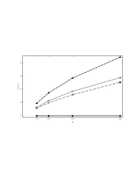
Figure 3: Scaling of the norm of the minimal control matrix required to achieve stability for various organizations: global (solid, black), local (dashed, black), hierarchy (solid, gray) and multihierarchy (dashed, gray) as a function of N. The hierarchical organizations are chosen with $r=0.5$ and branching ratio 2.

Fig. 3 shows the norm of the control matrix C as a function of N for these values, as given by the Frobenius norm [12], ${\left|C\right|}=\sqrt{\sum_{ij}{\left|C_{ij}\right|}^{2}}$. It shows that the global control can stabilize the system with the smallest control matrix, as expected since it does not act (unnecessarily) on the higher modes, which are already stable. The local control requires the largest matrices. The hierarchical cases are intermediate, with the multihierarchy being slightly better. This figure can also be viewed as a stability diagram: for each organization, below the line the control matrix is too small to stabilize the system, while above it the system is stable.

Notice the difference between the behaviors of the hierarchy and multihierarchy. Both provide effective ways of giving information to the agents about dynamics at different length scales, but the multihierarchy as described above is able to match perturbations at any scale and any location on the array. It also has the flexibility of combining information from different parents.

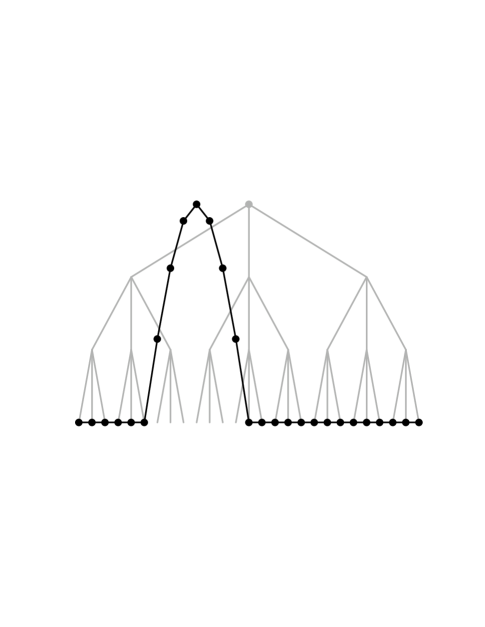
Figure 4: A localized perturbation for a chain with 27 elements (black) superimposed on the hierarchical organization with 3 levels and branching ratio 3 (gray). This perturbation cuts across a major organizational division of the hierarchy, between agents 9 and 10. The perturbation is nonzero only for agents 7 through 13, inclusive.

Figure 5: Forces acting on each agent when the chain is started in the configuration shown in Fig. 4 (and with zero velocity) when the maximum of the perturbation is set to $u_{10}=1$. The arrows show the forces produced using the multihierarchical control, while the individual points show the forces when the hierarchical control is used. In both cases, the agents use the maximum amplitude in the lowest mode estimated by their ancestors to determine their control response. System parameters are $\alpha=1$, $f=0.08$ and $s=1$ so this system is well within the stable regime.

For example, if the agents respond to the maximum amplitude estimate reported by any ancestors, the multihierarchy will be better able to respond to perturbations that cross organizational boundaries in the hierarchical organizations. This is illustrated in Fig. 5, which depicts the forces acting on each agent for a localized perturbation shown in Fig. 4. Near the maximum of the perturbation, both organizations respond nearly equally since the local value of the perturbation gives the largest amplitude estimate. However, for agents further away, we see the multihierarchy provides a stronger response since it is more effective at recruiting those agents to help push against the perturbation. Because the multihierarchy is able to focus effort at the most appropriate scale and location, we can expect it will provide a variety of more effective control strategies than the hierarchy.

5 Realistic Smart Matter

Traditional control theory and the discussion in the previous sections assume the existence of good models of the system. In real systems however, the values of the displacements given by sensors and of the actuator forces might be imperfect. Thus the agent’s knowledge of the dynamics of the system is only approximate.

These differences between theoretical models and actual systems have many causes. For example, any large scale manufacturing process leads to artifacts whose functional properties are distributed around a mean with dispersion $\sigma$, so that the information from sensors and the forces exerted by actuators will differ from the actual values according to the dispersion in their properties. This view is appropriate for devices manufactured in large quantities (e.g., as in many proposed applications of MEMS) but less so for unique structures or artifacts in different specific environments (such as control for large structures such as buildings).

Another source of imperfections is due to the “smart dust” approach in which control elements are scattered throughout a structure [9]. In such a situation the local environment of each of the elements won’t be constant through the system thus introducing a random modulation of their properties.

Finally, imperfections or unknown variations in physical characteristics of system mean the agents fit to an incorrect model of the dynamics.

In all these cases, the entries of the control matrix, C, in Eq. 2 would also deviate from their ideal values. In this section we investigate the consequences for stability of this randomization of the control matrix, both in general terms and for the example of the elastic array.

5.1 Stability

To investigate the consequences of realistic systems departing from the idealized models, we consider the average behavior of smart matter given an ensemble specifying uncertain knowledge about parameters entering the M matrix. For the sake of treating a very general case, we assume as little knowledge about these parameters as possible. This implies that all matrices can be considered, and that there is no particular basis for choosing one over the other. This is the class of the so-called random matrices, in which all such matrices are equally likely to occur. Matrices in this class have each entry obtained from a random distribution with a specified mean and variance. By taking this approach, we can make general statements about the stability of these systems as the number of components and degrees of freedoms grows.

To do this, we need to determine the average behavior of the largest eigenvalue of random matrices. The precise value of the eigenvalue with the largest real part, $\lambda_{1}$, of the matrix M depends on the particular choice of the entries. Methodologically, the study of the general behavior of these matrices is performed by examining the average properties of the class that satisfies all the known information about them. A class of plausible matrices is determined by the amount of information one has. The net results of these considerations is that the full control dynamics can be written as in Eq 2, but with the matrix M given by the sum of an ideal part and a random part

$${M=\tilde{M}+R}$$

(33)

both of which are influenced by the choice of control organization.

The eigenvalues of M are related to the eigenvalues of $\tilde{M}$ and R. For example, when the matrices are symmetric or else have non-negative entries, the largest eigenvalue is real and $\lambda_{1}$ is bounded by

$${\tilde{\lambda}_{N}+\lambda^{{\left(R\right)}}_{1}{\leq}\lambda_{1}{\leq}\tilde{\lambda}_{1}+\lambda^{{\left(R\right)}}_{1}}$$

(34)

where $\tilde{\lambda}_{N}$ is the smallest eigenvalue of the matrix $\tilde{M}$. Other types of matrices have more complicated relations concerning the largest eigenvalue but in most cases stability will be related to the behavior of the eigenvalues of R.

The eigenvalues of random matrices have been studied for a number of cases. They show surprising regularities that we can use to discuss the stability properties of realistic systems. In the case of random symmetric matrices whose entries have a positive mean value, on average, the largest eigenvalue is given by [8]

$${\lambda^{{\left(R\right)}}_{1}={\left(N-1\right)}\mu+\sigma^{2}/\mu}$$

(35)

where $\mu$ is the expected value of the entries in R, which we assume to be positive. Moreover, the actual values (as opposed to the average) of $\lambda_{1}$ are normally distributed around this value with variance $2\sigma^{2}$. When added to $\tilde{M}$ this implies that as the size of the system grows, most such matrices will have positive largest eigenvalue, thus making the control unstable. The case of asymmetric matrices can also be treated [8, 20] to give

$${\lambda^{{\left(R\right)}}_{1}\sim N\mu}$$

(36)

but in general Eq. 34 will not hold, making it more difficult to give definite results for this case.

From these considerations, we can expect that random matrices are unstable whenever their size and the magnitude and variation of their entries are large. In terms of the corresponding organization, these corresponds to large systems, with many strong interactions among the agents. This prediction is tempered by the fact that in localized organizations so many of the matrix elements are zero so that even with strongly interacting agents they tend to be stable [15]. Which of these effects is dominant is determined by the organizational structure.

5.2 Control Organizations

We now describe how the predictions concerning random matrices apply to different control organizations.

5.2.1 Global

Since a global control fills the full matrix, the imperfections make the matrix random. Assuming for simplicity that the matrix R has entries all chosen from the same probability distribution with mean $\mu$ and variance $\sigma^{2}$, the full matrix M will have a mean given by

$${\bar{M}_{ij}=\tilde{M}_{ij}+\mu}$$

(37)

and each element has variance $\sigma^{2}$.

Since the largest eigenvalue of the ideal matrix is negative due to its stability under controls, as N gets large the upper bounds of Eq. 34 gets positive. This happens even in the case of moderate values of N, as the dispersion of the imperfection properties will make the right hand side positive.

5.2.2 Local

A local control matrix is diagonal, so symmetry is quite natural in contrast to the global case. For a diagonal matrix R, the largest eigenvalue is given by the largest diagonal component. Since theses are chosen from a random distribution with mean $\mu$, and variance $\sigma^{2}$, the relevant eigenvalues originate in the extrema of the distribution, and they are given by the extreme value distribution function. If the eigenvalues are normally distributed, the extrema will scale with N as [35] $\lambda^{{\left(R\right)}}_{1}\sim\sigma\sqrt{2\ln N}$, implying higher stability than the global case due to the slow growth with N of $\lambda^{{\left(R\right)}}_{1}$. This scaling is independent of the value of $\mu$ provided it does not grow rapidly with N. The extrema of other distributions also grow quite slowly compared to N [35], showing that the increased stability of the local architecture as compared with the global is a general property, provided the matrix elements come from distributions with the same mean and variance.

5.2.3 Hierarchies and Multihierarchies

Suppose now that the system has a hierarchical structure of depth d and average branching ratio, b. In this case, the strength of the interaction between any two agents decreases with their ultrametric distance. Specifically, the interaction strength, i.e., the size of the element in the control matrix, will be taken to be $r^{h}$, with h the number of hierarchy levels that separate the two agents.

Detailed treatment of the properties of random matrices with hierarchical structure remains an open problem. Nevertheless, a good qualitative insight is obtained by ignoring this detailed structure except for its effect on the mean and variance of the distribution from which the matrix elements are selected. The size of the matrix is given by $N=b^{d}$ and the mean of the non-diagonal terms is

$${\mu={{\sum_{h=1}^{d}b^{h-1}{\left(b-1\right)}r^{h}}\over{\sum_{h=1}^{d}b^{h-1}{\left(b-1\right)}}}={{{\left(rb\right)}^{d}-1}\over{b^{d}-1}}\hskip 2.65pt{{r{\left(b-1\right)}}\over{rb-1}}}$$

(38)

The nature of the organization depends on whether the total interaction is dominated by neighboring agents or distant ones. The first case amounts to restricting r to be $r{<}1/b$. This choice makes the decreasing interaction strength between agents overwhelm the increase in their number as higher levels in the hierarchy are considered. In this situation when N is large Eq. 38 becomes $\mu={{r{\left(b-1\right)}}\over{{\left(1-rb\right)}N}}$, which implies that as N grows the mean goes to zero, leading to a stable system because of Eq. 36. However, if fluctuations in the coupling strength were taken into account, some of the matrices could still become unstable.

In the second case, $r{>}1/b$. This implies that in the large N limit the average becomes

$${\mu=r^{d}{{r{\left(b-1\right)}}\over{rb-1}}={{r{\left(b-1\right)}}\over{rb-1}}N^{{{\ln r}\over{\ln b}}}}$$

(39)

Note that since $-1{<}{{\ln r}\over{\ln b}}{<}0$, $\mu$ goes to zero as the size of the matrix grows, but in slower fashion than the case above. Nevertheless, this subtle difference in convergence to zero amounts to a qualitative difference in the stability of the system. To see this, notice that Eq. 36 implies that the largest eigenvalue of a random matrix grows as $\mu N$, which increases with N for this value of $\mu$, thus leading to instability when the system gets large enough. The growth in largest eigenvalue with the size of the system is exhibited in Fig. 6 for a particular choice of parameters. Notice that the system becomes unstable for $d{\geq}5$. Given these results we see that the size of the matrix for which this instability takes place is much larger than the one in the absence of a hierarchy of interactions.

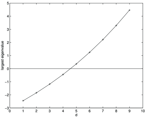
Figure 6: Plot showing the growth of the largest eigenvalue of a hierarchical random matrix with branching ratio $b=2$ and $r=0.55$ as a function of $d=\log_{2}n$. The diagonal elements were chosen to be $-3$. The points are the theoretically predicted values based on Eq. 38 and lie very close to the computed eigenvalues shown by the solid line.

Therefore, the largest eigenvalue will be similar to the behavior of the global case with a renormalization of the $\mu$ given by Eq. 38. Thus, a hierarchical control system is more stable than the global one but less so than the local case, for given interaction strength.

The multihierarchy organization matrix has a structure similar to the hierarchical case, but different in the sense that the entries are centered around the diagonal. This greater symmetry does not affect their values and therefore one gets the same qualitative behavior as for the hierarchy. A more detailed analysis of the different structures would be required to distinguish the behavior of these two organizations.

5.3 Example: The Imperfect Elastic Array

Elucidating the factors that dominate the behavior of random matrices for different organizations requires looking at particular instances. To see how imperfections affect the control of the elastic array, we consider the three sources of imperfections that arise in such systems and assume the errors they introduce are multiplicative. The sensors at the j^th location gives its reading of the local value as $u^{{\rm meas}}_{j}$. Because of its imperfect nature, this reading will differ from the actual value, $u_{j}$, by an amount $u^{{\rm meas}}_{j}=u_{j}{\left(1+r_{j}\right)}$, where $r_{j}$ represents the random imperfection of the sensor. Similarly for the actuators, the actual force, $f^{{\rm actual}}_{i}$ will differ from the nominal one, $f_{i}$, by

$${f^{{\rm actual}}_{i}=f_{i}{\left(1+e_{i}\right)}}$$

(40)

where $e_{i}$ represents the random imperfection of the actuator. The last source of imperfection has to do with the unknown variation in physical characteristics of the system to be controlled. This translates in having control matrix entries differ from the ideal values, $C_{ij}$ by $C^{{\rm computed}}_{ij}=C_{ij}{\left(1+\rho_{ij}\right)}$.

Combining all these factors gives

$${f^{{\rm actual}}_{i}=-s\sum C_{ij}{\left(1+r_{j}\right)}{\left(1+e_{i}\right)}{\left(1+\rho_{ij}\right)}u_{j}\equiv-s\sum_{j}C^{{\rm actual}}_{ij}u_{j}}$$

(41)

which we can write as $C^{{\rm actual}}_{ij}=C_{ij}{\left(1+\epsilon_{ij}\right)}$ where $\epsilon_{ij}$ includes contributions from all the sources of errors. If we suppose that the deviations from the nominal values are independent random values, but there is no systematic bias, then the $\epsilon_{ij}$ can be viewed as random variables with zero mean and some standard deviation we denote by $\sigma$. The introduction of errors can make the matrix $C^{{\rm actual}}_{ij}$ asymmetric, even though the ideal case is symmetric. For the full control dynamics governed by the matrix M, the value of $M_{jk}$ will vary randomly with an average value

$${A_{jk}+C_{jk}}$$

(42)

and standard deviation $\sigma C_{jk}$.

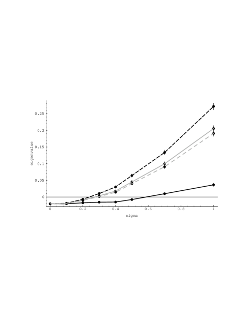
Figure 7: Effect of noise on the expected value of the largest eigenvalue, for $N=8$, $\alpha=1$, $f=0.8$ and controls with $s=0.7$ as a function of $\sigma$ for asymmetric multiplicative noise with zero mean and standard deviation $\sigma$. The organizations are global (solid, black), local (dashed, black), hierarchy (solid, gray) and multihierarchy (dashed, gray). For the hierarchical cases, we have $r=0.5$ and a branching ratio of two. The error bars give the standard error estimate of the mean, based on 1000 samples. Eigenvalues above zero indicate situations where the noise makes the system unstable, on average.

Fig. 7 shows the behavior of the expected value of the largest eigenvalue for a particular case with different organizations. The local control is most sensitive to the noise. This is contrary to what one might expect from analyses based on the connectivity of the matrices and is due to larger matrix elements, shown in Fig. 3, being more important than the degree of connectivity in the matrices.

These comparisons used the same set of random matrices for each organization, thus allowing a detailed pairwise comparison [27] of their relative performance independent of the variation due to different choices of the noise matrices. This shows that the difference in the behavior of the organizations is statistically much more significant than appears from the error bars in the figure.

Fig. 7 shows the behavior of the average of $\lambda_{1}$. Another measure of the consequence of imperfection is the fraction of cases that are unstable at each value of $\sigma$. This shows the same qualitative behavior of the organizations typically becoming unstable in the same order as shown for the average value.

This example exhibits the phenomenon of instability brought about by the system size, the interconnectivity of the control organization and the variance in the imperfections.

6 The Effect of Delays

In our discussion, we assumed that the agents were able to act instantaneously on the physical system. This is appropriate when the control elements (sensors, actuators and computations) operate rapidly compared to the relevant physical time scales of the unstable system. On the other hand, delays could arise from a variety of causes. For instance, there could be communication delays, in which case larger organizational structures, e.g., global, would have more delay than local ones. There could also be different communication delays for different agents as for example depending on their ultrametric distance in a hierarchy. However, while passing information through multiple levels of managers in a hierarchical organization may introduce additional delays in the information, for controlling physical devices this may not be much of a problem: the information aggregated over larger spatial scales corresponds to lower frequency behaviors which are less sensitive to delays.

On the other hand, if the main delay is in activation of the actuators, e.g., due to their inertia, then the delays could be more significant and fairly similar among the organization choices. A final possibility is that delays arise from the computation time required to determine the response to the given sensor inputs. This is not likely to be a problem for the simple control mechanisms discussed here but could be more significant if more complex strategies are used, especially if the agents include expectations of the behavior of other agents in their evaluations.

The behavior of the system with delays in the control can be analyzed most readily by assuming that all delays in the information are the same so Eq. 2 becomes

$${{{d^{2}{\bf u}{\left(t\right)}}\over{dt^{2}}}=-\Gamma{\bf\dot{u}}{\left(t\right)}+A{\bf u}{\left(t\right)}-C{\bf u}{\left(t-\tau\right)}}$$

(43)

where $\tau$ is the delay. That is, the control decisions are made based on a delayed value for the displacements. In this case the stability analysis is similar to that given above but results in a more complicated criterion. Specifically, suppose ${\bf u}{\left(t\right)}={\bf u}_{0}e^{\Lambda t}$ then we have

$${{\left(\Lambda^{2}I+\Gamma\Lambda I-A+Ce^{-\Lambda\tau}\right)}{\bf u}_{0}=0}$$

(44)

This has a solution only when the matrix is singular, i.e., when

$${\det{\left(\Lambda^{2}I+\Gamma\Lambda I-A+Ce^{-\Lambda\tau}\right)}=0}$$

(45)

This is a generalization of the eigenvalue criterion for the case with no delays, and is a so-called exponential-polynomial [2]. Unlike the dispersion relation in the undelayed case, this generally has an infinite number of complex solutions. Stability corresponds to having the real parts of all the solutions being nonpositive.

As an example, consider the case of the chain for the lowest mode ${\bf e}^{{\left(1\right)}}$ and assume the control matrix is such that this is an eigenvector of both A and C, with eigenvalues $\lambda^{{\left(A\right)}}$ and $\lambda^{{\left(C\right)}}$, respectively. By comparison, the dynamics with no delays is governed by $M=A-C$ with eigenvalue $\lambda=\lambda^{{\left(A\right)}}-\lambda^{{\left(C\right)}}$. In that case the criterion becomes

$${\Lambda^{2}+\Gamma\Lambda-\lambda^{{\left(A\right)}}+\lambda^{{\left(C\right)}}e^{-\Lambda\tau}=0}$$

(46)

For a simple analysis, consider the effect of a small delay, so $e^{\Lambda\tau}\approx 1-\Lambda\tau$ near the largest solutions. Then we have

$${\Lambda^{2}+{\left(\Gamma-\lambda^{{\left(C\right)}}\tau\right)}\Lambda-\lambda=0}$$

(47)

This effectively amounts to a decrease in the damping, but is otherwise the same as the condition leading to Eq. 5 for the case without delays.

When the delays prevent achieving stability, more sophisticated control algorithms will be required. For example, instead of a least squares fit to delayed values, the agents could use some averaging of different estimates of the size of the first mode, or attempt to extrapolate to the current state of the system. These sophisticated control strategies can be helpful, but some caution is required since they can also introduce additional instabilities [21].

6.1 Example: Elastic Array with Control Delays

In the chain example, $\lambda^{{\left(C\right)}}=s$ is positive so to first order, a delay decreases the damping a bit but does not change the stability properties, provided this decrease does not make the overall damping negative, i.e., as long as $s\tau{<}\Gamma$. While this argument is only valid for small delays, it shows how delays in the information available to the agents can lead to instability. Note that we require $s{\geq}\lambda^{{\left(A\right)}}$ to have stability even with no delays in the control. Thus these requirements restrict $\Gamma/\tau{>}s{\geq}\lambda^{{\left(A\right)}}$ and suggest there is no stable control beyond $\tau{>}\Gamma/\lambda^{{\left(A\right)}}$. This analysis for a single mode can also apply to other modes of the system. However, higher modes, i.e., those with smaller or even negative (in the case of modes that are stable even without control) values of $\lambda^{{\left(A\right)}}$ can tolerate larger delays than the lowest mode. Hence stability is determined by the behavior of the lowest mode, as is the situation when there are no delays. A more complete analysis of the stability [2] gives only a small correction to this criterion as long as the delays are small. An interesting observation from this criterion is that at least some damping is essential for the system to be stable with even the smallest delay.

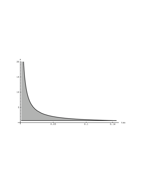
Figure 8: The gray region shows the stable combinations of control force, given by s, and delay $\tau$, for $N=8$, $\alpha=1$ and $f=0.8$ with $\Gamma=0.1$. Stability requires the control to be at least $s{\geq}f-f^{{\left(1\right)}}_{crit}=0.679$ even with no delay. The upper limit is close to $s{\leq}\Gamma/\tau$. For $\tau{>}0.147$ there is no stable control.

An example is show in Fig. 8. The dynamical equations with delays can also be solved directly [2, 32, 24] to exhibit the behavior of the system when the control is delayed.

7 Explosive Transient Growths

Maintaining stability is an important goal, but there remains the possibility of large transient growth even when system is stable. That is, the displacements could become large at intermediate time scales before eventually damping out. This means that for controlling these systems, stability is necessary but may not be sufficient to guarantee that small perturbations never produce large amplitudes which could couple to nonlinearities and damage the system.

This problem arises when the matrix M governing the system has some eigenvectors that are nearly parallel. For symmetric matrices, where the eigenvectors are always orthogonal, this problem never occurs. For instance, many physical systems, such as the elastic array we have considered, have physical forces that are symmetric. This leads to a symmetric matrix A provided the masses of the components are equal, as we assumed in the case of the elastic array. More general unequal masses, or the addition of an asymmetric random control matrix due to imperfections could lead to nearly parallel eigenvectors in some control organizations. Moreover, there are important systems, such as fluid motion [30], where the physical interactions themselves can give rise to asymmetric matrices with nearly parallel eigenvectors.

To illustrate the consequence of nearly parallel eigenvectors on the transient behavior of a mechanical system with a stable fixed point consider a two dimensional case where the eigenvectors are $v_{1}={\left(1,0\right)},\hskip 2.65ptv_{2}={\left(1,\epsilon\right)}$, with eigenvalues $\lambda_{1}=-1\hskip 2.65pt\hbox{\rm and}\hskip 2.65pt\lambda_{2}=-5$. The dynamics are determined by $v{\left(t\right)}=av_{1}e^{\lambda_{1}t}+bv_{2}e^{\lambda_{2}t}$. Thus, for an initial condition where these two vectors nearly cancel, such as $a=1\hskip 2.65pt\hbox{\rm and}\hskip 2.65ptb=-1$, the evolution becomes $v{\left(t\right)}={\left(e^{-t}-e^{-5t},\hskip 2.12006pt-\epsilon e^{-5t}\right)}$ with magnitude $e^{-t}\sqrt{1-2e^{-6t}+e^{-8t}{\left(1+\epsilon^{2}\right)}}$. An example of the resulting dynamics is shown in Fig. 9.

Figure 9: Example of a giant transient for the two dimensional example with $\epsilon=0.01$. Although the system is asymptotically stable, its magnitude becomes many times larger than the initial perturbation before eventually decaying.

The possibility of this large transient growth is not commonly appreciated in analyses of system stability, and gives another criterion to check for in designing control organizations. For our example of multiplicative noise in the elastic array, the local control, which is diagonal, will not give rise to any asymmetries. However the global control, and also to some extent, the hierarchical organizations, can be sensitive to errors in this way.

Figure 10: Example of transient growth possible with asymmetric noise. In this case, the magnitude of the displacement vector is shown on the vertical axis with $N=8$, $\alpha=1$ and $f=0.8$ with $\Gamma=0.005$ with global control of $s=0.7$. The horizontal axis depicts time. Initially the system was at rest with a displacement vector of magnitude 0.05. Subsequently, the displacement vector reaches a magnitude of about 1.5, about 30 times larger than the initial state. For larger times, the oscillations continue with gradually decreasing amplitude showing that the system is indeed stable.

An example of the elastic array with asymmetric multiplicative noise giving a large transient growth is shown in Fig. 10. This system is stable, i.e., the oscillations eventually approach zero. However, the initial perturbation is greatly amplified before this eventual decrease, thus providing a situation where the system could couple to undesirable nonlinear behaviors, or overwhelm the maximum forces available from the actuators, even though the stability criterion is satisfied.

8 Discussion

In this paper, we studied the behavior of control organizations for unstable physical systems. We have shown how a hierarchical organization is a reasonable compromise between rapid local responses with simple communication and the use of global knowledge. This holds not only in ideal situations but also when imperfections and delays are present in the system. This work illustrates the consequence of the strong physical embedding of the computational agents.

We also introduced a new control organization, the multihierarchy, and showed it is somewhat better than a hierarchy in achieving stability, while having in addition a position invariant response which allows for the control of disturbances at appropriate scale and location.

An important characteristic of smart matter is the distinction between the use of physical information vs. social or computational information: when the control consists in minor adjustments and the communication is fast, agents can respond based on the physical states of the system. In other cases, e.g., when there are long delays or very strong actuation forces, it may be important for the agents to respond based on expectations for what the other agents are likely to do. This leads to the possibility of more complex dynamics, as has been seen in computational ecosystems [21]. Equally interesting there is regime between these extremes where the dynamics will significantly couple the networks of computational interactions and the physical substrate thus giving rise to novel behaviors.

Although the behaviors of distributed controls were illustrated in the context of a one-dimensional elastic array, the results apply to a wider range of situations. First because this oscillatory model describes a variety of physical systems, these results hold for two and three dimensional materials, as well as giving some insight into the control of nonlinear systems. Thus from knowledge of the physical properties of the system to be controlled one is able to characterize its controllability with distributed computation.

Second, we have treated imperfections independently for each agent. As the number of agents increases and they are closer together, this assumption may fail. For example, a defect at a certain location may affect all the agents close to it giving rise to short range correlations in the entries of the random matrix describing the control. Longer range correlations may be due to systematic mistakes in the agents’ models of the system. While random matrices with correlations can be studied and show qualitatively similar behaviors, in our case short range correlations will have no effect on the stability. This is because stability is determined by the behavior long wavelengths excitations of the physical system, and these low modes will not be affected by short range correlations.

Third, this methodology applies to other performance metrics. These include a variety of goals for smart matter: stability; small transient growth; robustness against imperfections in physical model, sensors, actuators and delays; simplicity of programming control; low communication and power use; and minimal cost of the devices. Generally, we will desire some combination of these goals. Since these goals can conflict, a major challenge for control design is how to manage them. This points to the need for a simple framework to express trade-offs among these goals. For large distributed systems, one appropriate mechanism is given by computational markets [33, 6], with the advantage of simplicity, robustness and scalability.

We close by pointing out some open issues that remain to be studied. One is the question of intermittent failures of actuators and sensor noise. Unlike the static imperfections we treated, they require stochastic controls [1]. This raises the question of how different organizations respond to ongoing noise, or sudden changes (e.g., a stuck actuator). The latter example amounts to a sudden switch from one static imperfect system to another, to which our results should apply. Another issue is the reaction time scales of different organizations, and whether there are more appropriate control mechanisms to deal with the large transient growth that we discussed.

Other questions that remain to be addressed include dynamically adjusting organization based on changes. For example, as components are assembled into larger structures the relative performance of different organizations may change, leading to the evolution of different structures [19]. Similarly some parts of the structure may be more active than others, requiring locally different organizational structures. In these cases agents may have less overall information than we assumed in our study (e.g., knowledge of nominal global modes and their location within the overall structure) leading to further possibilities to explore. These include different, and dynamically changing, organizational structures as the agents learn about the nature of the system they work with. Another question is to what extent the physical propagating modes in the underlying substrate can be used as a communication channel to convey properties of the environment, thereby limiting the need for fabricating additional wires.

Controlling smart matter brings together domains of physics and distributed computing. As a result, the physical characteristics of the system to be controlled strongly influence the effectiveness of the computational organizations. Smart matter thus provides a fertile ground for the interplay between dynamics in Euclidean space and processing in abstract spaces.

9 Acknowledgement

We have profited from many useful comments by Mark Yim. This work was partially supported by ONR Contract No. N00014–94-C–0096

References

- [1] K. J. Astrom. Introduction to Stochastic Control Theory. Academic Press, 1970.
- [2] R. Bellman and K. L. Cooke. Differential-Difference Equations. Academic Press, New York, 1963.
- [3] A. A. Berlin. Towards Intelligent Structures: Active Control of Buckling. PhD thesis, MIT, Dept. of Electrical Engineering and Computer Science, 1994.
- [4] A. A. Berlin, H. Abelson, N. Cohen, L. Fogel, C. M. Ho, M. Horowitz, J. How, T. F. Knight, R. Newton, and K. Pister. Distributed information systems for MEMS. Technical report, Information Systems and Technology (ISAT) Study, 1995.
- [5] Janusz Bryzek, Kurt Petersen, and Wendell McCulley. Micromachines on the march. IEEE Spectrum, pages 20–31, May 1994.
- [6] Scott H. Clearwater, editor. Market-Based Control: A Paradigm for Distributed Resource Allocation. World Scientific, Singapore, 1996.
- [7] E. H. Durfee. Special section on distributed artificial intelligence. In IEEE Transactions on Systems, Man and Cybernetics, volume 21. IEEE, 1991.
- [8] Z. Furedi and K. Komlos. The eigenvalues of random symmetric matrices. Combinatorica, 1:233–241, 1981.
- [9] K. J. Gabriel. Microelectromechanical systems (MEMS). A World Wide Web Page with URL http://eto.sysplan.com/ETO/MEMS/index.html, 1996.
- [10] Les Gasser and Michael N. Huhns, editors. Distributed Artificial Intelligence, volume 2. Morgan Kaufmann, Menlo Park, CA, 1989.
- [11] Natalie S. Glance and Tad Hogg. Dilemmas in computational societies. In V. Lesser, editor, Proc. of the 1st International Conference on Multiagent Systems (ICMAS95), pages 117–124, Menlo Park, CA, June 1995. AAAI Press.
- [12] G. H. Golub and C. F. Van Loan. Matrix Computations. John Hopkins University Press, Baltimore, MD, 1983.
- [13] Steven R. Hall, Edward F. Crawley, Jonathan P. How, and Benjamin Ward. Hierarchic control architecture for intelligent structures. J. of Guidance, Control, and Dynamics, 14(3):503–512, 1991.
- [14] J. A. Hartigan. Representation of similarity matrices by trees. Journal of the American Statistical Association, 62:1140–1158, 1967.
- [15] T. Hogg, B. A. Huberman, and Jacqueline M. McGlade. The stability of ecosystems. Proc. of the Royal Society of London, B237:43–51, 1989.
- [16] Tad Hogg and Bernardo A. Huberman. Controlling chaos in distributed systems. IEEE Trans. on Systems, Man and Cybernetics, 21(6):1325–1332, November/December 1991.
- [17] Jonathan P. How and Steven R. Hall. Local control design methodologies for a hierarchic control architecture. J. of Guidance, Control, and Dynamics, 15(3):654–663, 1992.
- [18] B. A. Huberman, editor. The Ecology of Computation. North-Holland, Amsterdam, 1988.
- [19] Bernardo A. Huberman and Tad Hogg. Communities of practice: Performance and evolution. Computational and Mathematical Organization Theory, 1(1):73–92, 1995.
- [20] F. Juhasz. On the asymptotic behavior of the spectra of non-symmetric random (0,1) matrices. Discrete Mathematics, 41:161–165, 1982.
- [21] J. O. Kephart, T. Hogg, and B. A. Huberman. Dynamics of computational ecosystems. Physical Review A, 40:404–421, 1989.
- [22] Victor Lesser, editor. Proc. of the 1st International Conference on Multiagent Systems (ICMAS95), Menlo Park, CA, 1995. AAAI Press.
- [23] James V. Mahoney and David T. Clemens. Position-invariant hierarchical image analysis. preprint, 1995.
- [24] George Marsaglia, Arif Zaman, and John C. W. Marsaglia. Numerical solution of some classical differential-difference equations. Mathematics of Computation, 53(187):191–201, 1989.
- [25] Kai Nagel. Life times of simulated traffic jams. Intl. J. of Modern Physics C, 5(4):567–580, 1994.
- [26] M.S. El Naschie. Stress, Stability and Chaos in Structural Engineering. McGraw Hill, 1st edition, 1990.
- [27] William H. Press, Brian P. Flannery, Saul A. Teukolsky, and William T. Vetterling. Numerical Recipes. Cambridge Univ. Press, Cambridge, 1986.
- [28] A. C. Sanderson and G. Perry. Sensor-based robotic assembly systems: Research and applications in electronic manufacturing. Proc. of IEEE, 71:856–871, 1983.
- [29] Elisabeth Smela, Olle Inganas, and Ingemar Lundstrom. Controlled folding of micrometer-size structures. Science, 268:1735–1738, 1995.
- [30] Lloyd N. Trefethen, Anne E. Trefethen, Satish C. Reddy, and Tobin A. Driscoll. Hydrodynamic stability without eigenvalues. Science, 261:578–584, July 30 1993.
- [31] David M. Upton. A flexible structure for computer controlled manufacturing systems. Manufacturing Review, 5(1):58–74, 1992.
- [32] G. S. Virk. Runge-Kutta method for delay-differential systems. IEEE Proceedings, 132 D(3):119–123, May 1985.
- [33] Carl A. Waldspurger, Tad Hogg, Bernardo A. Huberman, Jeffery O. Kephart, and W. Scott Stornetta. Spawn: A distributed computational economy. IEEE Trans. on Software Engineering, 18(2):103–117, February 1992.
- [34] Shih-Ho Wang and Edward J. Davison. On the stabilization of decentralized control systems. IEEE Trans. on Automatic Control, AC-18(5):473–478, 1973.
- [35] Michael Woodroofe. Probability with Applications. McGraw-Hill, New York, 1975.