[

Density Waves in a Transverse Electric Field

Abstract

In a quasi-one-dimensional conductor with an open Fermi surface, a Charge or a Spin Density Wave phase can be destroyed by an electric field perpendicular to the direction of high conductivity. This mechanism, due to the breakdown of electron-hole symmetry, is very similar to the orbital destruction of superconductivity by a magnetic field, due to time-reversal symmetry.

]

It is well-known that superconductivity becomes unstable in the presence of an external magnetic field and that the transition temperature $T_{c}$ is reduced. This is due to the breakdown of time-reversal symmetry which leads to orbital frustration. More precisely, in the presence of a vector potential ${\bf A}$, a single electron wave function gets a phase shift ${e\over\hbar}\int{\bf A}d{\bf l}={e\over\hbar}\int{\bf A}{\bf v}dt$ and a Cooper pair acquires a phase shift ${2e\over\hbar}\int{\bf A}d{\bf l}$. This dephasing of the Cooper pair is at the origin of the reduction of $T_{c}$ [1, 2].

It is also known that this magnetostatic effect has an electrostatic analog. An electron moving in a static potential $V$ acquires a phase ${e\over\hbar}\int Vdt$. This is the electrostatic Aharonov-Bohm effect[3]. Although the sign of this phase is not changed with the velocity, it is changed with the sign of the carrier. That is why one expects that an electron-hole pair will get a phase shift ${2e\over\hbar}\int Vdt$ exactly like the Cooper pair gets the phase ${2e\over\hbar}\int{\bf A}d{\bf l}$ . In other words, the magnetic field breaks the time reversal symmetry and the scalar potential breaks the electron-hole symmetry. We show in this letter that, in an appropriate geometry, this dephasing of the electron-hole pair may lead to the suppression of the Charge Density Wave (CDW) or Spin Density Wave (SDW) state by an applied electric field. This field destroys the DW ordering in a very similar way that the magnetic field destroys superconductivity (fig. 1).

The physical properties of CDW’s and in particular their elastic properties have been extensively studied. The main goal was to describe the effect of an electric field parallel to the chains and transport properties (like non-linear transport or conversion of current at the boundaries)[5, 6]. The effect described here is specific of a quasi-1D system, where the hopping integral $t_{\perp}$ between chains plays an essential role. The Fermi surface is open and the electric field is applied along the direction perpendicular to the chains. Although difficult to observe experimentally, this new effect could be measurable in low $T_{c}$ Density Wave systems, for example in the SDW state of Bechgaard salts. The effect described here is purely thermodynamical. We do not describe any effect related to nonlinear transport.

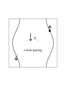
FIG. 1.: a) In a magnetic field $H_{z}$, two electrons move in opposite directions and accumulate opposite phases, leading to the destruction of Cooper pairing. b) In a transverse electric field $E_{y}$, an electron ($\bullet$) and a hole ($\circ$) move in opposite directions and accumulate opposite phases, leading to the destruction of the electron-hole pairing.

Consider for simplicity a two-dimensional open Fermi surface, in a plane ($k_{x},k_{y}$) . $k_{x}$ indicates the direction of highest conductivity . An electric field $E_{y}$ is applied along the $y$-direction. Using a tight-binding dispersion relation linearized around the Fermi level in the x direction of high conductivity, the Hamiltonian writes: ($\hbar=1$ throughout the paper):

$${\cal H}({E_{y}})=v_{F}(|k_{x}|-k_{F})+t_{\perp}(k_{y}b)-eE_{y}y$$ (1)

$v_{F}$ is the Fermi velocity. The periodic function $t_{\perp}(p)$ describes the warping of the Fermi surface. As an example, we will take $t_{\perp}(p)=-2t_{b}\cos(p)$ where $t_{b}$ is the transfer integral between chains. In such a case, the Fermi surface has perfect nesting at wave vector ${\bf Q}_{0}=(2k_{F},\pi/b)$ so that, in zero electric field, a DW is stable below a critical temperature $T_{c}$ given by a BCS form $T_{c}=T_{c}(E=0)=E_{0}\exp(-1/gN(\epsilon_{F}))$. $g$ is the coupling constant and $N(\epsilon_{F})$ is the density of states at the Fermi level.

We now follow the lines of the usual semi-classical (eikonal) picture used by Gor’kov[1] in the case of a magnetic field on a superconductor. This approximation consists in replacing $y$ in eq.(1) by its semi-classical zero field expression

$$y_{\alpha}(k_{y},x)=\alpha{bt_{\perp}^{\prime}(k_{y}b)\over v_{F}}x$$ (2)

$\alpha=\pm 1$ describes the two sides of the Fermi surface. As a result, the wave function writes:

$$\phi_{{\bf k},\alpha}({\bf r})={1\over\sqrt{S}}\exp[i{\bf kr}+i\varphi(x,0)]$$ (3)

$S$ is the area. As explained in the introduction, the additional phase factor:

$$\varphi(x,x^{\prime})=i\alpha{eE_{y}\over v_{F}}\int_{x^{\prime}}^{x}y_{\alpha}(k_{y},x)dx$$ (4)

has indeed the form $e\int Vdt$ ($\hbar=1$) since $V=eE_{y}y$ and $dt=dx/v_{F}$. The Green function for an electron on the right (left) side of the Fermi surface, written in a mixed representation[4] is:

$$G_{\alpha}(x,x^{\prime},k_{y},\omega_{n},E_{y})=G_{\alpha}^{0}(x,x^{\prime},k_{y},\omega_{n})e^{i\varphi(x,x^{\prime})}$$ (5)

$\omega_{n}$ are the Fermion Matsubara frequencies. $G_{\alpha}^{0}$ is the $E_{y}=0$ Green function.

We now write the linearized integral equation which describes the stability of the DW phase, at the wave vector ${\bf Q}=(Q_{x},Q_{y})$ ,

$${\Delta({\bf Q},x)\over g}=\int\nolimits dx^{\prime}K({\bf Q},x,x^{\prime})\Delta({\bf Q},x^{\prime})$$ (6)

where, in the mixed representation, the kernel K of this one-dimensional equation is given by:

$$K({\bf Q},x,x^{\prime})=T\sum_{\omega_{n}>0}\int\nolimits{dk_{y}b\over{2\pi}}G_{+}^{0}(x,x^{\prime},k_{y},\omega_{n})\times$$ (7)

$$G_{-}^{0}(x^{\prime},x,k_{y}-Q_{y},\omega_{n})\exp[iQ_{\parallel}(x-x^{\prime})]\exp[i\phi]$$ (8)

where

$$\phi={eE_{y}\over v_{F}}\int_{x^{\prime}}^{x}[y_{+}(k_{y},x)+y_{-}(k_{y}-Q_{y},x)]dx$$ (9)

This kernel has the same structure as the superconducting kernel in a magnetic field. The phase factor (9) which has the form $2e\int Vdt$ plays a role similar to the phase factor induced by the vector potential in the case of a magnetic field $\exp[2ie\int{\bf A}d{\bf l}]$ ($\hbar=1$).

Inserting eq. 2 into the phase factor (9), performing the Matsubara sum and the integral in eq. 8 one finds that, close to the nesting vector ${\bf Q}_{0}$, the gap equation writes:

$${\Delta({\bf Q},x)\over g}=\int_{u>d}{du\over x_{T}\sinh({u\over x_{T}})}\times$$ (10)

$$J_{0}[{2t_{b}\over v_{F}}u(q_{y}+{2eE_{y}bx\over v_{F}})]\Delta({\bf Q},x+u)$$ (11)

where $q_{y}=\pi/b-Q_{y}$. $x_{T}=v_{F}/(2\pi T)$ is the thermal length . $d$ is a lower cut-off such that $1/g=\ln(\pi dT_{c}/v_{F})$. In order to discuss the DW stability criterion, we first derive the linearized Ginzburg-Landau equation from the gap equation (6,8) [1]. Expanding $\Delta(x+u)$ and the Bessel function $J_{0}$ for small separation $u$, it is then straightforward to get the equation for the spatial variation of the order parameter $\Delta({\bf r})=\Delta\exp(-i{\bf Q}_{0}{\bf r})f({\bf r})$, where $f=f({\bf r})$ obeys:

$$[{1\over 4}{\partial^{2}\over\partial x^{2}}+{t_{b}^{2}b^{2}\over 2v_{F}^{2}}({\partial\over\partial y}+{2ieE_{y}x\over v_{F}})^{2}+{4\pi^{2}T_{c}^{2}\over 7\zeta(3)v_{F}^{2}}(1-{T\over T_{c}})]f=0$$ (12)

or, by gauge transformation:

$$[-{1\over 4}({\partial\over i\partial x}+{2eV\over v_{F}})^{2}+{t_{b}^{2}b^{2}\over 2v_{F}^{2}}{\partial^{2}\over i\partial y^{2}}+{4\pi^{2}T_{c}^{2}\over 7\zeta(3)v_{F}^{2}}(1-{T\over T_{c}})]f=0$$ (13)

This linearized Ginzburg-Landau equation is identical to the one which describes the superconducting order parameter in a magnetic field. The analogy with the magnetic field effect on superconductivity is clearly seen from the structure of the Hamiltonian (1) which is very similar to the Hamiltonian in a magnetic field ${\bf H}=(0,0,H_{z})$ perpendicular to the plane. Using the Landau gauge ${\bf A}=(0,-H_{z}y,0)$, one gets

$${\cal H}(H_{z})=v_{F}(|(k_{x}+eH_{z}y)|-k_{F})+t_{\perp}cos(k_{y}b)$$ (14)

The similar form of the two Hamiltonians clearly reflects the physical description presented above. The absolute value in eq.(14) simply reflects that, on the left side of the Fermi surface, the electron travels in the same direction in the presence of $E_{y}$ or $H_{z}$, while, on the right side, it travels in opposite directions (fig. 1). This analogy between the two Hamiltonians is of course due to the quasi-1D structure of the Fermi surface and originates from the linearization of the dispersion relation along x. Using the different gauge ${\bf A}=(0,Hx,0)$, it may be seen that the superconducting kernel contains the phase factor

$$\exp[i\int_{x^{\prime}}^{x}t_{\perp}(p-eHbx)-t_{\perp}(p-q_{y}+eHbx)dx]$$ (15)

Small $x$ expansion of the periodic factors $t_{\perp}$ directly leads to an expression similar to eq.(9).

From standard manipulation of eq.(13) [7], we find that the critical temperature decreases linearly as $T_{c}(E)=T_{c}(1-E/E_{c})$. A simple extrapolation of this linear behavior down to zero temperature[8] defines a critical field $E_{c}$ at which the DW completely disappears. $E_{c}$ is given by

$$2ebE_{c}={8\sqrt{2}\pi^{2}T_{c}^{2}(0)\over 7\zeta(3)t_{b}}$$ (16)

This relation has a simple meaning. Noting that $T_{c}\propto\Delta$, the critical field is such that $2eE_{y}\xi_{y}\simeq\Delta$: the potential energy of the electron-hole pair is of the order of the binding energy of the pair $\Delta$ ( $\xi_{y}\simeq{v_{y}\over\Delta}\simeq{t_{b}b\over\Delta}$ is the transverse coherence length). Below $T_{c}$, the CDW order parameter should exhibit a non-uniform structure similar to the mixed state of superconductors.

Expression (16) for the critical field shows that the destruction of the DW is a 2D effect. This effect disappears when the coupling $t_{b}$ between chains vanishes. The critical field is smaller when $t_{b}$ is large. On the other hand, it should not be too large so that the Fermi surface remains open and that a DW can still exist.

The above derivation has been presented in the case of a perfect nesting. An imperfectly nested DW can also been destroyed by an electric field. We have checked that the GL equation has the same structure in the case of imperfect nesting.

We see from eq. (16) that the effect of the electric field is easier to detect in DW systems with low critical temperature so that a small field can be applied. Using the parameters of Bechgaard salts [9], one can estimate $E_{c}$ of the order of $E_{c}=25T_{c}^{2}V/cm$. In order to have an electric field as small as possible, one should use a salt with a very small $T_{c}$. A favorable situation to observe this new effect is to apply pressure on the SDW of a Bechgaard salt like $(TMTSF)_{2}PF_{6}$, in order to reduce its critical temperature ($10K$ at ambient pressure[9]). The linear decrease of $T_{c}(E)$ could then be observed in a typical electric field of order $10V/cm$.

An experimental difficulty to observe this effect may be due to the screening of the electric field in the metallic phase and along the transition line so that rather than measuring directly the decrease of $T_{c}(E)$ (by measures of the resistance R(T) at different fields for example), it may be more appropriate to work at very low temperature well below $T_{c}$ so that the DW order parameter is maximum and the screening is minimum, and to apply the electric field. Another possibility may be to apply a voltage to the sample with contacts so that a small current will flow long the $y$ direction.

During the completion of this work, I have been aware of a preprint by M. Hayashi and H. Yoshioka, who have treated a similar problem[10].

Acknowledgments: I benefited from useful discussions with H. Bouchiat, N. Dupuis, M. Gabay, P. Lederer, B. Reulet and H. Schulz.

REFERENCES

- [1] L.P. Gorkov, Zh. Eksp. Teor. Fiz. 36,1918 (1959) (Sov. Phys. JETP 36, 1364 (1959)).
- [2] A.A. Abrikosov, Sov. Phys. JETP 36, 1364 (1959).
- [3] S. Washburn, H. Schmid, D. Kern and R.A. Webb, Phys. Rev. Lett. 59, 1791 (1987)
- [4] L.P. Gorkov and A.G. Lebed, J. Phys. Lett. 43, L433 (1984).
- [5] For a review on Charge and Spin Density Waves see for example: G. Grüner, Rev. Mod. Phys. 60, 1129 (1988); 66, 1 (1994); L.P. Gorkov and G. Grüner, Charge Density Waves in Solids, in Modern Problems in Condensed Matter in Sciences, Vol. 2( (North-Holland 1989)
- [6] L.P. Gor’kov, JETP 59, 1057 (1985); N.P. Ong, G. Verma and K. Maki, Phys. Rev. Lett. 52, 663 (1984); D. Feinberg and J. Friedel, J. Phys. France 49, 485 (1988); H. Fukuyama ad P.A. Lee, Phys. Rev. 17, 535 (1978); P.A. Lee and T.M. Rice, Phys. Rev. 19, 3970 (1979).
- [7] see, e.g., D.R. Tilley and J.R.Tilley, Superfluidity and Superconductivity, Graduate student series in Physics, D.F. Brewer ed., Adam Hilger ltd. (1986)
- [8] The Ginzburg-Landau expansion is valid for
- [9] D. Jérome and H.J. Schulz, Adv. Phys. 31, 299 (1982).
- [10] M. Hayashi and H. Yoshioka, cond-mat/9609148, to appear in Phys. Rev. Lett.