Classical artificial two-dimensional atoms: the Thomson model

Abstract

The ring configurations for classical two-dimensional (2D) atoms are calculated within the Thomson model and compared with the results from ‘exact’ numerical simulations. The influence of the functional form of the confinement potential and the repulsive interaction potential between the particles on the configurations is investigated. We also give exact results on those eigenmodes of the system whose frequency does not depend on the number of particles in the system.

I Introduction

Recently, a detailed investigation of the ground state configurations of a finite two-dimensional (2D) classical system of charged particles, confined by a parabolic external potential, was made in Ref. [3]. It was found that the particles arranged themselves on rings. A study of the spectral properties of this classical system such as the energy spectrum, the eigenmodes, and the density of states was made in Ref. [4]. In both papers Monte Carlo simulations were used to study these classical atoms.

In the present paper we aim to obtain analytic results for these classical 2D atoms by using a model system: the Thomson model. Thomson proposed this classical model in 1904 in order to calculate the structure of the atom. [5] He was unable to obtain analytic results for the case of a real 3D atom and therefore constrained the particles to move in a plane. Together with the parabolic confinement potential this is now a model for the classical 2D atoms which were studied in Refs. [3] and [4]. A crucial ansatz in the Thomson model is that the particles arrange themselves in a ring structure. Next, Thomson puts as many particles as possible on a single ring, as allowed by stability arguments, and the rest of them are placed in the centre. By successive applying this approach he was able to construct the approximate atomic ring configurations.

Here we apply the Thomson model and compare the obtained configurations with those from the ‘exact’ numerical simulations of Ref. [3] and determine when the Thomson model breaks down. In a second step we generalize the Thomson model to: 1) general $r^{n}$ confinement potentials, and 2) different functional forms ($1/r^{n^{\prime}}$ and logarithmic) for the repulsive inter-particle potential.

This paper is organized as follows. The calculation to obtain the structure and the eigenfrequencies in the Thomson model is outlined in Section II. We compare the results for parabolic confinement and Coulomb repulsion with the previous results from ‘exact’ numerical simulations. Section III is devoted to the extensions of the Thomson model. In Section IV we give some analytical results for the eigenfrequencies of artificial atoms. Our conclusions and our results are summarized in Section V.

II The Thomson model

A General system

We study a system of a finite number, $N$, of charged particles interacting through a repulsive inter-particle potential and moving in two dimensions (2D). A confinement potential keeps the system together. We focus our attention on systems described by the Hamiltonian

$$H=\sum_{i=1}^{N}\frac{1}{2}m\omega_{0}^{2}\left(\frac{r_{i}}{\lambda}\right)^{n}+\frac{e^{2}}{\epsilon}\sum_{j>i}^{N}\frac{1}{|\vec{r}_{i}-\vec{r}_{j}|^{n^{\prime}}},$$ (1)

where $m$ is the mass of the particle, $\omega_{0}$ the radial confinement frequency, $e$ the particle charge, $\epsilon$ the dielectric constant of the medium the particles are moving in, and $\vec{r_{i}}=(x_{i},y_{i})$ the position of the particle with $r_{i}\equiv|\vec{r_{i}}|$. For convenience, we will refer to our charged particles as electrons, keeping in mind that they can also be ions with charge $e$ and mass $m$. We can write the Hamiltonian in a dimensionless form if we express the coordinates, energy, and force in the following units

$$r_{0}=(e^{2}/\epsilon)^{1/(n+n^{\prime})}\alpha^{-1/(n+n^{\prime})},\\$$ (3)

$$E_{0}=(e^{2}/\epsilon)^{n/(n+n^{\prime})}\alpha^{n^{\prime}/(n+n^{\prime})},\\$$ (4)

$$F_{0}=(e^{2}/\epsilon)^{(n-1)/(n+n^{\prime})}\alpha^{(n^{\prime}+1)/(n+n^{\prime})},$$ (5)

where $\alpha=\frac{{}_{1}}{{}^{2}}m\omega_{o}^{2}/\lambda^{n}$. All the results will be given in reduced form, i.e., in dimensionless units. In such units the Hamiltonian becomes

$$H=\sum_{i=1}^{N}r_{i}^{n}+\sum_{j>i}^{N}\frac{1}{|\vec{r}_{i}-\vec{r}_{j}|^{n^{\prime}}}.$$ (6)

Thus, the energy is only a function of the number of particles $N$, the power of the confinement potential $n$ and the power of the interaction potential $n^{\prime}$. For $n=2$ and $n^{\prime}=1$ this system reduces to the one studied in Refs. [3] and [4]. The numerical values for the parameters $r_{0}$ and $E_{0}$ for some typical experimental systems like electrons in quantum dots,[6] electron bubbles on a liquid Helium surface,[7] and ions trapped in Penning and Paul traps[8] were given in Ref. [3] for the case of parabolic confinement and Coulomb repulsion.

In the Thomson model one obtains the groundstate configurations of this system by making the following assumption: the $N$ electrons are arranged at equal angular intervals around the circumference of a circle of radius $a$. Then one investigates the stability of this configuration. With other words, small displacements of the electrons out of their equilibrium have to remain small in time. Solving the equations of motion in polar coordinates to first order in these displacements, we obtain an equation which determines the eigenfrequencies $\omega$ of the system

$$\left((n+n^{\prime})\frac{I(n^{\prime})}{2^{n^{\prime}+1}a^{n^{\prime}+2}}S_{N}+L_{k}-L_{0}+(n-2)\Omega^{2}-\omega^{2}\right)\left(N_{0}-N_{k}-\omega^{2}\right)=\left(M_{k}-2\Omega\omega\right)^{2},$$ (7)

where $\Omega$ is a constant angular velocity with which the whole system rotates around its centre, $I(n^{\prime})=n^{\prime}$, and

$$S_{N}=\sum_{j=1}^{N-1}\frac{1}{\sin^{n^{\prime}}({j\pi}/{N})},$$ (9)

$$L_{k}=\frac{I(n^{\prime})}{(2a)^{n^{\prime}+2}}\sum_{j=1}^{N-1}\frac{\cos(2kj\pi/N)}{\sin^{n^{\prime}+2}(j\pi/N)}\left(n^{\prime}\sin^{2}(j\pi/N)+1\right),$$ (10)

$$N_{k}=\frac{I(n^{\prime})}{(2a)^{n^{\prime}+2}}\sum_{j=1}^{N-1}\frac{\cos(2kj\pi/N)}{\sin^{n^{\prime}}(j\pi/N)}\left((n^{\prime}+1)\cot^{2}({j\pi}/{N})+1\right),$$ (11)

$$M_{k}=n^{\prime}\frac{I(n^{\prime})}{(2a)^{n^{\prime}+2}}\sum_{j=1}^{N-1}\sin\frac{2kj\pi}{N}\frac{\cos(j\pi/N)}{\sin^{n^{\prime}+1}(j\pi/N)}.$$ (12)

where $k$ is an integer between $0$ and $N-1$. The derivation of Eq. (7) is straightforward and proceeds along the lines given by Thomson[5] for the case of $n=2$ and $n^{\prime}=1$. How many frequencies yields this equation? From the onset we notice that if we replace $k$ by $N-k$ in Eq. (7), the values of $\omega$ differ only in sign, and thus results in the same frequencies. Consequently all the values of $\omega$ can be obtained by taking only $k=0,1,\ldots,(N-1)/2$ if $N$ is odd, or $k=0,1,\ldots,N/2$ if $N$ is even. Thus, if $N$ is odd there are $(N+1)/2$ equations of the type (7). For $k=0$, $M_{k=0}=0$, and Eq. (7) reduces to a quadratic equation, which implies that the number of roots of these $(N+1)/2$ equations equals $4\times(N+1)/2-2=2N$, i.e. the number of degrees of freedom of the system, as should be. For $N$ even, there are $N/2+1$ equations. But $M_{k}=0$ for $k=0$ and $k=N/2$, and thus two of these reduce to quadratics. Consequently, the number of roots is $4\times\left(N/2+1\right)-4=2N$. Thus in both cases the number of roots is equal to $2N$, the number of degrees of freedom of the electrons in the plane of motion and therefore all eigenfrequencies are obtained from Eq. (7).

B Parabolic confinement and Coulomb repulsion

Let’s consider the case of parabolic confinement ($n=2$) and Coulomb repulsion between the electrons ($n^{\prime}=1$). Eq. (7) for the eigenfrequencies becomes

$$\left(\frac{3}{4a^{3}}S_{N}+L_{k}-L_{0}-\omega^{2}\right)\left(N_{0}-N_{k}-\omega^{2}\right)=\left(M_{k}-2\Omega\omega\right)^{2}.$$ (13)

If we take $\lambda=1$ in Eq. (1) the frequency is expressed in the unit $\omega^{\prime}=\omega_{0}/\sqrt{2}$.

Figure 1 shows the eigenfrequencies squared for $N=1,2,3,4,5$ and $6$ for zero angular velocity, i.e. $\Omega=0$. Notice that the lowest non zero eigenfrequency decreases and in fact for $N=6$ we find that $\omega^{2}<0$ indicating that the single ring configuration is no longer stable. However, it is possible to stabilize the system by placing electrons in the centre. If we put $p$ electrons in the centre of the ring, Eq. (7) is modified into

$$\left((n+n^{\prime})\frac{I(n^{\prime})}{2^{n^{\prime}+1}a^{n^{\prime}+2}}S_{N}+L_{k}-L_{0}+\frac{(n^{\prime}+2)I(n^{\prime})p}{a^{n^{\prime}+2}}+(n-2)\Omega^{2}-\omega^{2}\right)\left(N_{0}-N_{k}-\omega^{2}\right)$$ (14)

$$=\left(M_{k}-2\Omega\omega\right)^{2}.$$ (15)

From this equation we obtain the minimum value for $p$ which is needed in order to make a ring of $N_{out}$ electrons stable. For parabolic confinement and Coulomb repulsion between the particles we find the condition

$$p>f(k,N_{out})\equiv\frac{a^{3}}{3}\left(L_{0}-L_{k}\right)-\frac{S_{N_{out}}}{4}+\frac{a^{3}}{3}\frac{M_{k}^{2}}{N_{0}-N_{k}},$$ (16)

which must be satisfied for every $k$. We introduce $f(N_{out})=\max_{k\in[0,N)}$ and $p$ equals the integer which is just larger than $f(N_{out})$. Figure 2 shows the function $f(N_{out})$. For $p$ larger than one, the $p$ inner electrons in principle cannot be in the same point, i.e. in the centre. They will repel each other until they balance the confinement potential. The Thomson model assumes, as is approximately the case, that the $p$ electrons around the centre exert the same force as resulting from $p$ charges placed at the centre. As an example we consider the case of $N_{out}=12$. For an outer ring of $12$ electrons, Eq. (16) requires that $7$ electrons are inside (this result can be read off from Fig. 2). But $7$ electrons cannot form a single ring, but will arrange themselves as a ring of $6$ with one at the centre. Thus the system of $19$ electrons will consist of an outer ring of $12$, an inner ring of $6$ and one electron at the centre.

Following the above procedure we can construct a table of Mendeljev and compare it with the results of the ‘exact’ numerical simulations. [3] This is done by finding the distribution of the electrons when they are arranged in what we may consider to be the simplest way, i.e. when the number of rings is a minimum. The number of electrons in the outer ring $N_{1}$ will then be determined by the equation

$$N-N_{1}=f(N_{1}).$$ (17)

The value of $N_{1}$ as obtained from this equation is not an integer and consequently we have to take the integral part of this value. To obtain $N_{2}$, the number of electrons in the second ring, we solve

$$N-N_{1}-N_{2}=f(N_{2}).$$ (18)

We continue in this way until there remain less than $6$ electrons. This procedure results into Table I. This table of Mendeljev for the Thomson model is compared with the ‘exact’ table of Ref. [3]. The configurations for which the Thomson model gives the wrong results are printed in italics. Notice that this model is capable to predict most of the configurations correctly. For systems with many electrons ($N>35$) the Thomson model starts to fail. However even in this case the number of rings is still predicted correctly until $N<50$. The reason for this difference is that in the Thomson model the configurations are found by using a stability argument, while in Ref. [3] they were found by a minimalization of the energy using Monte Carlo simulations. Here we will not compare the energy as obtained from the Thomson model with the result given in Ref. [3]. We found that the energy in the Thomson model for $N>6$ deviates strongly from the ‘exact’ results which is due to the assumption that all inner electrons are placed at the centre.

III Extensions of the Thomson model

A Effect of the confinement potential

It turned out that for parabolic confinement and Coulomb repulsion the maximum number of particles on the inner ring is $5$. Now we want to investigate how the confinement potential influences the possible configurations. For simplicity, we take $n^{\prime}=1$ for the inter-particle repulsion, i.e. Coulomb repulsion.

From Eq. (15) we obtain the minimal value for $p$ which stabilizes a ring of $N_{out}$ electrons

$$p>\frac{a^{3}}{3}\left(L_{0}-l_{k}\right)-\frac{n+1}{12}S_{N}+\frac{a^{3}}{3}(2-n)\Omega^{2}+\frac{a^{3}}{3}\frac{M_{k}^{2}}{N_{0}-N_{k}},$$ (19)

and this inequality must hold for every $k$. Notice that only for $n=2$, i.e. parabolic confinement, this stability condition does not depend on the angular velocity $\Omega$. For a linear confinement potential ($n=1$) each configuration will become unstable for sufficient large $\Omega$, while for $n>2$ every configuration can be stabilized if the system rotates fast enough. To get an idea of the influence of the confinement potential on the configurations we limit ourselves to the case $\Omega=0$. Following the same procedure as used in previous section we find the table of Mendeljev (Table II). The results presented in Table II are a good first approximation to the ‘exact’ results for the considered $N$-values. Figure 3 shows the maximum number of electrons on the inner, second, …, sixth ring as function of $n$. Notice that for a linear confinement potential the inner ring can support a maximum of $3$ electrons which is much smaller than in the case of a parabolic confinement. For confinement potentials with $n>2$ it’s just the opposite, more electrons can be fitted on the rings without destabilizing them.

In the limit of $n\rightarrow\infty$ the confinement potential becomes a hard wall potential, i.e. $V(r)=0\;\;(r<\lambda),\infty\;\;(r>\lambda)$. We found numerically that the maximum number of particles on each of the rings keeps increasing with $n$. This clearly signals the breakdown of the Thomson model in this limit because from ‘exact’ numerical simulations (see Ref.[3]) with a hard wall circular potential it is known that, with increasing number of electrons, inner rings are formed. We can understand this as follows. In the Thomson model the groundstate configurations are found using a stability argument, so only inner rings are formed to stabilize the outer electrons. For a hard wall potential, there is no confining force for $r<\lambda$, thus no inner electrons are needed. All the electrons form one ring at $r=\lambda$, but this is not the configuration with the minimum value of the energy.

For completeness, we mention that recently Farias and Peeters [9] studied a system of $4$ electrons in a Coulomb type of confinement and found different configurations depending on the strength of the Coulomb confinement potential. This together with the present results indicate that the number of electrons on each ring are not universal but can be strongly influenced by the type and strength of the confinement potential.

B Effect of the inter-particle interaction potential

Now we investigate the effect of the functional form of the interaction potential between the electrons on the groundstate configurations. For simplicity, we consider here a parabolic confinement potential ($n=2$).

First we can extend the inter-particle potential to a logarithmic interaction. To obtain Eqs. (7) and (15) we used $1/r^{n^{\prime}}$ as the inter-particle potential. These equations are obtained from the law of Newton which contains the force. Because the derivative of $\ln r$ equals $1/r$ these equations are therefore also valid for a logarithmic inter-particle interaction where we have to take $n^{\prime}=0$ and $I(0)=1$.

In Table III, we give the table of Mendeljev as obtained from the generalized Thomson model using a logarithmic and a $1/r^{2}$ interaction, and compare the results with the one for a Coulomb interaction (Table III). For the $1/r^{2}$ interaction we find that with increasing number of electrons more electrons have to be placed at the centre than for the case of Coulomb interaction in order to stabilize the outer ring. Therefore the resemblance with the ‘exact’ table of Mendeljev will not be as good as for the case of Coulomb interaction. Indeed, the effect of the assumption that all inner electrons are placed at the centre will be larger. For the logarithmic interaction the opposite is found. Fewer electrons have to be placed at the centre and in this case the Thomson model should work very well. Figure 4 shows the maximum number of electrons on the inner, second, …, sixth ring as function of $n^{\prime}$. Notice that the maximum occupation number of the different rings decreases with increasing $n^{\prime}$.

For $n^{\prime}\rightarrow\infty$ we found numerically $N_{1}=4$ and for all the outer rings $N=6$. Also in this limit we do not expect that the Thomson model gives the correct results, because the inter-particle interaction becomes extremely short range, i.e. they are delta function like. Classically the electrons can sit very close to each other and thus will occupy the $r\approx 0$ region where the confinement potential is zero. As a consequence, such a system is similar to the case of an infinite 2D Wigner lattice where the particles form a hexagonal lattice, i.e. each electron has $6$ neighbours, and no ring structure is expected. Similar results were recently obtained [10] for a screened Coulomb interaction $e^{-\kappa r}/r$ using a molecular dynamics simulation approach. With increased screening, i.e. larger $\kappa$, structural transitions were found in which the ring configurations changed abruptly and in the limit of very large $\kappa$ a 2D Wigner type lattice was formed in the centre of the classical 2D atom.

IV Eigenfrequencies independent of the number of electrons

Figure 1 suggests that in the case of parabolic confinement and Coulomb repulsion there are three eigenfrequencies independent of the number of electrons (see also Ref. [4]). The existence and value of these eigenfrequencies can be obtained analytically. 1) For any axial symmetric system the system as a whole can rotate, which leads to an eigenfrequency $\omega=0$. 2) The Hamilton equation of motion yields $\dot{v}_{xi}=-nx_{i}\left(x_{i}^{2}+y_{i}^{2}\right)^{n/2-1}+n^{\prime}\sum_{j_{j\neq i}}(x_{i}-x_{j})/{r_{ij}^{n^{\prime}+2}}$. Now consider the centre of mass $\vec{R}=\sum_{i}\vec{r}_{i}$ which satisfies the differential equation

$$\frac{d^{2}R_{x}}{dt^{2}}=\sum_{i}\dot{v}_{xi}=-n\sum_{i}x_{i}\left(x_{i}^{2}+y_{i}^{2}\right)^{n/2-1},$$ (20)

and of course the same for $R_{y}$. Notice that Eq. (20) is independent of $n^{\prime}$. Thus only for a parabolic confinement potential the above equation reduces to $d^{2}R_{x}/dt^{2}=-2R_{x}$ and a twofold degenerate vibration of the centre of mass with eigenfrequency $\omega=\sqrt{2}$ is obtained. This frequency is independent of the number of electrons and independent of the inter-particle potential which is a consequence of the generalized Kohn theorem.[11] 3) For the mean square radius $R^{2}=\sum_{i}\left(x_{i}^{2}+y_{i}^{2}\right)$ we find

$$\frac{d^{2}R^{2}}{dt^{2}}=-(n+n^{\prime})\sum_{i}\left(x_{i}^{2}+y_{i}^{2}\right)^{n/2}+n^{\prime}H+2T,$$ (21)

with $T=\sum_{i}\left(\dot{x}_{i}^{2}+\dot{y}_{i}^{2}\right)$ the total kinetic energy. For parabolic confinement, i.e. $n=2$, there is a breathing mode with frequency $\omega=\sqrt{2+n^{\prime}}$ which is independent of the number of electrons. The existence of the breathing mode does not depend on the functional form of the inter-particle potential, but its value does.

V Conclusions and summary

The Thomson model, a model for classical 2D atoms, was investigated and the groundstate configurations were obtained. The results are valid for repelling particles with arbitrary mass and charge. First, we deduced within the Thomson model a table of Mendeljev for parabolic confinement and Coulomb repulsion between the electrons and compared it with the results from ‘exact’ Monte Carlo simulations. [3] The Thomson model correctly predicts the configurations for $N<36$. This table was constructed using stability arguments: the eigenfrequencies of the 2D atom are calculated and determined when one of them becomes imaginary in order to find the maximum number of electrons on the rings.

Knowing that the Thomson model is a rather good model to predict the configurations of classical 2D atoms we investigated the effect of a $r^{n}$-confinement potential. Only for parabolic confinement the configurations do not depend on the angular velocity for rotation of the total system. For a linear confinement potential the configuration becomes unstable if the system rotates too fast, while for $n>2$ every configuration may be stable if the system rotates fast enough. We also found that the maximum number of allowed electrons on each ring is an increasing function of $n$, i.e. it increases with the steepness of the confinement potential.

We extended the Thomson model to a $1/r^{n^{\prime}}$-type and to logarithmic interaction between the electrons and found the groundstate configurations. Here we found that with increasing $n^{\prime}$, i.e. for shorter range of inter-particle interaction, fewer electrons can be put on a ring.

We showed that there are three eigenfrequencies which are independent of the number of electrons in the case of parabolic confinement. The zero frequency mode which is a consequence of the axial symmetry of the system. We found that only for a parabolic confinement potential the frequencies of the vibration of the centre of mass and the breathing mode are independent of the number of electrons. The value of the latter does depend on the functional form of the inter-particle potential.

VI Acknowledgments

This work is supported by the Human Capital and Mobility network Programme No. ERBCHRXT 930374. B.P. and F.M.P. are supported by the Flemish Science Foundation (FWOVlaanderen).

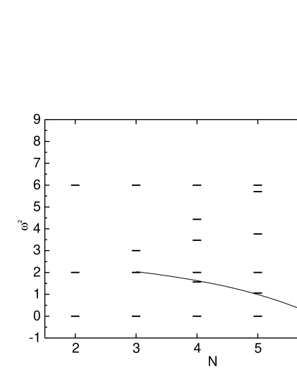
FIG. 1.: The eigenfrequencies squared for $N=2,3,4,5,6$ for $\Omega=0$.

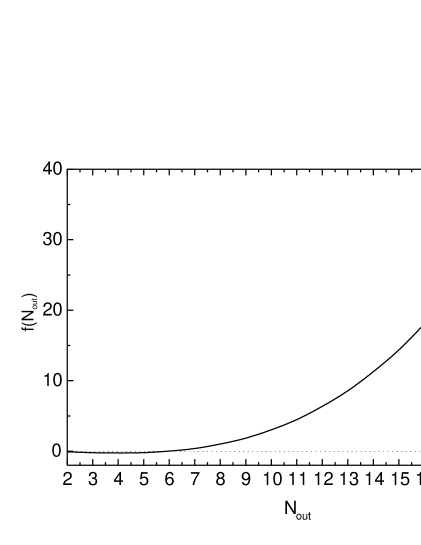
FIG. 2.: The number of electrons $f(N_{out})$ needed in the centre of the system in order to stabilize a ring of $N_{out}$ electrons.

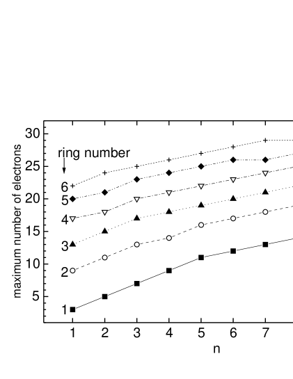
FIG. 3.: The maximum number of electrons on the inner, second, …, sixth ring as function of the power of the confinement potential ($n$) for the case of Coulomb repulsion between the electrons.

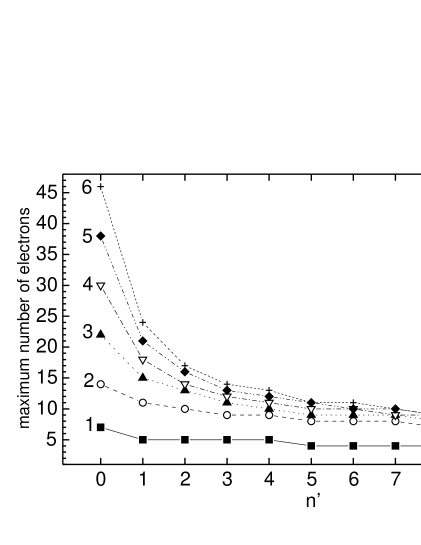
FIG. 4.: The maximum number of electrons on the inner, second, …, sixth ring as function of the power of the inter-particle interaction ($n^{\prime}$) for the case of a parabolic confinement potential. $n^{\prime}=0$ corresponds to a logarithmic interaction.

TABLE I.: Table of Mendeljev for classical 2D atoms. The results as obtained from the Thomson model are compared with the ‘exact’ results from the Monte Carlo simulations of Ref. [3].

N	Thomson	Monte Carlo	N	Thomson	Monte Carlo
1	1	1	26	3,9,14	3,9,14
2	2	2	27	4,9,14	4,9,14
3	3	3	28	4,10,14	4,10,14
4	4	4	29	5,10,14	5,10,14
5	5	5	30	5,10,15	5,10,15
6	1,5	1,5	31	5,11,15	5,11,15
7	1,6	1,6	32	1,5,11,15	1,5,11,15
8	1,7	1,7	33	1,6,11,15	1,6,11,15
9	2,7	2,7	34	1,6,12,15	1,6,12,15
10	2,8	2,8	35	1,6,12,16	1,6,12,16
11	2,9	3,8	36	1,7,12,16	1,6,12,17
12	3,9	3,9	37	2,7,12,16	1,7,12,17
13	4,9	4,9	38	2,7,13,16	1,7,13,17
14	4,10	4,10	39	2,8,13,16	2,7,13,17
15	5,10	5,10	40	2,8,13,17	2,8,13,17
16	5,11	1,5,10	41	2,9,13,17	2,8,14,17
17	1,5,11	1,6,10	42	3,9,13,17	3,8,14,17
18	1,6,11	1,6,11	43	3,9,14,17	3,9,14,17
19	1,6,12	1,6,12	44	4,9,14,17	3,9,14,18
20	1,7,12	1,7,12	45	4,9,14,18	3,9,15,18
21	2,7,12	1,7,13	46	4,10,14,18	4,9,15,18
22	2,7,13	2,8,12	47	5,10,14,18	4,10,15,18
23	2,8,13	2,8,13	48	5,10,15,18	4,10,15,19
24	2,9,13	3,8,13	49	5,11,15,18	4,10,15,20
25	3,9,13	3,9,13	50	1,5,11,15,18	4,10,16,20

TABLE II.: Table of Mendeljev for the Thomson model for various confinement potentials $r^{n}$.

N	n=1	n=2	n=3	n=10	N	n=1	n=2	n=3	n=10
3	3	3	3	3	14	1,4,9	4,10	4,10	14
4	1,3	4	4	4	15	1,4,10	5,10	4,11	15
5	1,4	5	5	5	16	1,5,10	5,11	5,11	16
6	1,5	1,5	6	6	17	1,5,11	1,5,11	5,12	17
7	1,6	1,6	7	7	18	1,6,11	1,6,11	6,12	1,17
8	2,6	1,7	1,7	8	19	2,6,11	1,6,12	7,12	2,17
9	2,7	2,7	1,8	9	20	2,7,11	1,7,12	7,13	3,17
10	2,8	2,8	1,9	10	21	2,7,12	2,7,12	1,7,13	4,17
11	3,8	2,9	2,9	11	22	2,8,12	2,7,13	1,8,13	4,18
12	3,9	3,9	2,10	12	23	3,8,12	2,8,13	1,9,13	5,18
13	1,3,9	4,9	3,10	13	24	3,8,13	2,9,13	1,9,14	6,18

TABLE III.: The groundstate configurations for logarithmic, Coulomb and $1/r^{2}$ interaction between the particles, as obtained within the Thomson model, as a function of the total number of particles $N$.

N	$-\ln r$	$1/r$	$1/r^{2}$	N	$-\ln r$	$1/r$	$1/r^{2}$
2	2	2	2	27	2,9,16	4,9,14	5,10,12
3	3	3	3	28	2,9,17	4,10,14	5,10,13
4	4	4	4	29	2,10,17	5,10,14	1,5,10,13
5	5	5	5	30	2,10,18	5,10,15	1,6,10,13
6	6	1,5	1,5	31	3,10,18	5,11,15	1,6,11,13
7	1,6	1,6	1,6	32	3,11,18	1,5,11,15	1,7,11,13
8	1,7	1,7	1,7	33	3,11,19	1,6,11,15	2,7,11,13
9	1,8	2,7	2,7	34	4,11,19	1,6,12,15	2,8,11,13
10	2,8	2,8	2,8	35	4,12,19	1,6,12,16	2,8,11,14
11	2,9	2,9	3,8	36	4,12,20	1,7,12,16	3,8,11,14
12	2,10	3,9	3,9	37	5,12,20	2,7,12,16	3,8,12,14
13	3,10	4,9	4,9	38	5,13,20	2,7,13,16	3,9,12,14
14	3,11	4,10	5,9	39	5,13,21	2,8,13,16	4,9,12,14
15	4,11	5,10	5,10	40	6,13,21	2,8,13,17	5,9,12,14
16	4,12	5,11	1,5,10	41	6,14,21	2,9,13,17	5,10,12,14
17	5,12	1,5,11	1,6,10	42	6,14,22	3,9,13,17	5,10,13,14
18	5,13	1,6,11	1,6,11	43	1,6,14,22	3,9,14,17	1,5,10,13,14
19	6,13	1,6,12	1,7,11	44	1,7,14,22	4,9,14,17	1,5,10,13,15
20	6,14	1,7,12	2,7,11	45	1,7,15,22	4,9,14,18	1,6,10,13,15
21	1,6,14	2,7,12	2,8,11	46	1,7,15,23	4,10,14,18	1,6,11,13,15
22	1,7,14	2,7,13	3,8,11	47	1,8,15,23	5,10,14,18	1,7,11,13,15
23	1,7,15	2,8,13	3,8,12	48	1,8,16,23	5,10,15,18	2,7,11,13,15
24	1,8,15	2,9,13	3,9,12	49	1,8,16,24	5,11,15,18	2,8,11,13,15
25	1,8,16	3,9,13	4,9,12	50	2,8,16,24	1,5,11,15,18	2,8,11,14,15
26	2,8,16	3,9,14	5,9,12	51	2,9,16,24	1,6,11,15,18	3,8,11,14,15

REFERENCES

- [1] Electronic mail: bpartoen@uia.ua.ac.be
- [2] Electronic mail: peeters@uia.ua.ac.be
- [3] V. M. Bedanov and F. M. Peeters, Phys. Rev. B 49, 2667 (1994).
- [4] V. A. Schweigert and F. M. Peeters, Phys. Rev. B 51, 7700 (1995).
- [5] J. J. Thomson, Philos. Mag. 7, 237 (1904).
- [6] Nanostructure Physics and Fabrication, edited by M. A. Reed and W. P. Kirk (Academic, Boston, 1989).
- [7] B. Lehndorff, J. Löhle, and K. Dransfeld, Surf. Sci. 229, 362 (1990); V. B. Shikin and E. V. Lebedeva, Pis’ma Zh. Eksp. Teor. Fiz. 57, 126 (1993) [JETP Lett. 57, 135 (1993)].
- [8] D. J. Wineland and W. M. Itano, Phys. Today 40 (6), 34 (1987); C. N. Cohen-Tannoudji and W. D. Philips, Phys. Today 43 (10), 33 (1990); W. Neuhauser, M. Hohenstatt, P. E. Toschek, and H. Dehmelt, Phys. Rev. A 22, 1137 (1980).
- [9] G. Farias and F.M. Peeters, Solid Stat. Commun. 100 (1996)
- [10] N. Studart and J. Pedro (private communications)
- [11] W. Kohn, Phys. Rev. 123, 1242 (1961); L. Brey, N. F. Johnson, and B. I. Halperin, Phys. Rev. B 40, 10 647 (1989); P. A. Maksym and T. Chakraborty, Phys. Rev. Lett. 65, 108 (1990); F. M. Peeters, Phys. Rev. B 42, 1486 (1990).