ITP-UH-22/96 September 1996

OUTP-9633S cond-mat/9610222

Exact solution of a $t$-$J$ chain with impurity

Gerald Bedürftig¹ , Fabian H.L. Eßler² and Holger Frahm^1
1Institut für Theoretische Physik, Universität Hannover
D-30167 Hannover, Germany
²Department of Physics, Theoretical Physics, Oxford University
1 Keble Road, Oxford OX1 3NP, Great Britain
ABSTRACT

We study the effects of an integrable impurity in a periodic $t$-$J$ chain. The impurity couples to both spin and charge degrees of freedom and has the interesting feature that the interaction with the bulk can be varied continuously without losing integrability. We first consider ground state properties close to half-filling in the presence of a small bulk magnetic field. We calculate the impurity contributions to the (zero temperature) susceptibilities and the low temperature specific heat and determine the high-temperature characteristics of the impurity. We then investigate transport properties by computing the spin and charge stiffnesses at zero temperature. Finally the impurity phase–shifts are calculated and the existence of an impurity bound state in the holon sector is established.

PACS-numbers: 71.27.+a  75.10.Lp  05.70.Jk  

1 Introduction

Theoretical investigations of strongly correlated electron systems have shown that the low temperature properties of such one dimensional systems have to be described in terms of a Luttinger liquid rather than a Fermi liquid. Of particular interest also from an experimental point of view are the transport properties of these systems in the presence of boundaries and potential scatterers. Several attempts have been made to describe such a situation: the transport properties of a 1D interacting electron gas in the presence of a potential barrier have been first studied using renormalization group techniques [1, 2]. Triggered by a more recent study of this problem by Kane and Fisher [3] different approaches such as boundary conformal field theory [4] and an exact solution by means of a mapping to the boundary sine-Gordon model [5, 6, 7, 8] have been applied to this problem. In particular the low temperature properties of magnetic (Kondo) impurities in a Luttinger liquid [9, 10, 11, 12] have been investigated in great detail. In the present work we will investigate the effects of a particular type of potential impurity in a Luttinger liquid (where both spin-and charge degrees of freedom are gapless) by means of an exact solution through the Quantum Inverse Scattering Method (QISM). Attempts to study effects due to the presence of impurities in many-body quantum system in the framework of integrable models have a long successful history [13, 14, 15, 16, 17, 18]. As far as lattice models are concerned the basic mechanisms underlying these exact solutions are based on the fact that the QISM allows for the introduction of certain “inhomogeneities”into vertex models without spoiling integrability. Two approaches are possible and have been studied for various models:
Since the ${\cal L}$-operators defining the local vertices satisfy a Yang-Baxter equation with an ${\cal R}$ matrix depending on the difference of spectral parameters only, one can build families for vertex models with site-dependent shifts of the spectral parameters. This has been widely used in solving models for particles with an internal degree of freedom by means of the nested Bethe Ansatz [19] and, more recently, also for the construction of systems with integrable impurities [16] (for a particularly simple case see [20]).
A second possibility is to introduce an impurity by choosing an ${\cal L}$-operator intertwining between different representations of the underlying algebra (possibly with an additional shift of the spectral parameter). This has first been used by Andrei and Johannesson to study the effect of a spin $S$ site in a spin-${1\over 2}$ Heisenberg chain [13]. Later this approach was used to study chains with alternating spins [14, 15].

Our work is based on the second approach. A novel feature as compared to [13] is the presence of a continuously varying free parameter describing the strength of the coupling of the impurity to the host chain. The presence of the free parameter is based on properties of the underlying symmetry algebra of the model, which in our case is the graded Lie algebra $gl(2|1)$ (see below).

Recently, vertex models and the corresponding quantum chains invariant under the action of graded Lie algebras have attracted considerable interest [21, 22, 23, 24, 25, 26, 27]. In addition to the well known supersymmetric $t$–$J$ model [29, 30, 31, 32, 33] (which is based on the fundamental three-dimensional representation of $gl(2|1)$) a model for electrons with correlated hopping has been constructed using the one-parametric family of four-dimensional representations of $gl(2|1)$ [34, 35, 36, 37, 38].

In this paper we study the properties of the supersymmetric $t$–$J$ model with one vertex replaced by an ${\cal L}$ operator acting on a four–dimensional quantum space. This preserves the supersymmetry of the model but at the same time lifts the restriction of no double occupancy present in the $t$–$J$ model at the impurity site. The free parameter associated with the four–dimensional representation of the superalgebra allows one to tune the coupling of the impurity to the host chain. Note that the present models allows for the study a situation which in some respects is more general than the ones mentioned above: the impurity introduced here couples to both spin- and charge degrees of freedom of the bulk Luttinger liquid. The extension of our calculation to the case of many impurities is straightforward (and will in fact be used in some parts of the paper).

The paper is organized as follows: In the following section we give a brief review of the Quantum Inverse Scattering Method and the Bethe Ansatz for $gl(2|1)$-invariant models. Then we study the ground state properties, low temperature specific heat and transport properties and show how they are affected by the presence of the impurity. Finally we compute the phase shifts acquired by the elementary excitations, holons and spinons, when scattered off the impurity.

2 Construction of the model

The impurity model is constructed by means of the graded version of the Quantum Inverse Scattering Method [39, 40, 41]. We start with the ${\cal R}$-matrix of the supersymmetric $t$-$J$ model [32]

$${\cal R}_{tJ}={\cal R}_{33}=\frac{\lambda}{\lambda+i}\Pi+\frac{i}{\lambda+i}1\ ,$$ (2.1)

with $\Pi^{a_{1}b_{1}}_{a_{2}b_{2}}=\delta_{a_{1}b_{2}}\delta_{a_{2}b_{1}}(-1)^{\epsilon_{b_{1}}\epsilon_{b_{2}}}$ being the graded permutation operator acting in the tensor product of two “matrix spaces” isomorphic to the three-dimensional “quantum space” space spanned by $(\uparrow,\downarrow,0)$ with the respective grading $\varepsilon_{\uparrow}=\varepsilon_{\downarrow}=1$ and $\varepsilon_{0}=0$. The corresponding $t$-$J$ ${\cal L}$-operator is given by ${\cal L}_{33}=\Pi{\cal R}_{33}$ and satisfies the following (graded) intertwining relation

In components this equations reads

$${\cal R}_{33}(\lambda-\mu)_{a_{2}c_{2}}^{a_{1}c_{1}}{\cal L}_{33}(\lambda)_{\alpha\gamma}^{c_{1}b_{1}}{\cal L}_{33}(\mu)_{\gamma\beta}^{c_{2}b_{2}}(-1)^{\varepsilon_{c_{2}}(\varepsilon_{c_{1}}+\varepsilon_{b_{1}})}={\cal L}_{33}(\mu)_{\alpha\gamma}^{a_{1}c_{1}}{\cal L}_{33}(\lambda)_{\gamma\beta}^{a_{2}c_{2}}(-1)^{\varepsilon_{a_{2}}(\varepsilon_{a_{1}}+\varepsilon_{c_{1}})}{\cal R}_{33}(\lambda-\mu)_{c_{2}b_{2}}^{c_{1}b_{1}}\ .$$ (2.2)

The monodromy matrix ${\cal T}_{tJ}$ is defined on the graded tensor product on quantum spaces and its matrix elements are given by

$${\cal T}_{tj}(\lambda)^{a\alpha_{1}\cdots\alpha_{L}}_{b\beta_{1}\cdots\beta_{L}}={\cal L}_{33}(\lambda)^{ac_{L}}_{\alpha_{L}\beta_{L}}{\cal L}_{33}(\lambda)^{c_{L}c_{L-1}}_{\alpha_{L-1}\beta_{L-1}}\cdots{\cal L}_{33}(\lambda)^{c_{2}b}_{\alpha_{1}\beta_{1}}(-1)^{\sum_{j=2}^{L}\left(\epsilon_{\alpha_{j}}+\epsilon_{\beta_{j}}\right)\sum_{i=1}^{j-1}\epsilon_{\alpha_{i}}}\ .$$ (2.3)

The hamiltonian of the $t$-$J$ model is then given as the logarithmic derivative of the transfer matrix $\tau(\lambda)=\mbox{str}[{\cal T}_{tJ}(\lambda)]:=\sum_{a=1}^{3}(-1)^{\epsilon_{a}}[{\cal T}_{tJ}(\lambda)]^{aa}$ at zero spectral parameter [32]

$${\cal H}_{tJ}=-i\frac{\partial}{\partial\lambda}\ln(\tau_{33})\Big{|}_{\lambda=0}-2{\cal N}_{e}=-\sum_{k=1}^{L}(\Pi_{k,k+1}-1)-2{\cal N}_{e}\ .$$ (2.4)

The ${\cal R}_{33}$-matrix can be constructed as the intertwiner of the three–dimensional fundamental representation of the superalgebra $gl(2|1)$. An impurity model can then be constructed in a way analogous to the spin-$S$ impurity in a spin-$\frac{1}{2}$ Heisenberg chain [13] by considering the intertwiner of the three–dimensional representation with the typical four–dimensional representation corresponding to an impurity site with four possible states ($\uparrow,\downarrow,\uparrow\downarrow=2,0$). In this way we obtain an ${\cal L}$-operator ${\cal L}_{34}$ with the same auxiliary space dimension as the ${\cal R}_{33}$-matrix satisfying the following equation:

The double line denotes the four–dimensional space $(\uparrow,\downarrow,2,0)$ with the respective grading $\varepsilon_{\uparrow}=\varepsilon_{\downarrow}=1$ and $\varepsilon_{2}=\varepsilon_{0}=0$. So double occupancy is possible at the impurity. The ${\cal L}_{34}$-matrix is given by

$${\cal L}_{34}=\frac{\lambda-i({\alpha\over 2}+1)}{\lambda+i({\alpha\over 2}+1)}+\frac{i}{\lambda+i({\alpha\over 2}+1)}{\cal L}\ ,$$ (2.5)

where ${\cal L}$, expressed in terms of projection operators (the so called ‘Hubbard Operators’) $X^{ab}=|a\rangle\langle b|$ with $a,b=\uparrow,\downarrow,2,0$, is given by

$${\cal L}=\left(\begin{array}[]{ccc}X_{2}^{\downarrow\downarrow}+X_{2}^{00}&-X_{2}^{\downarrow\uparrow}&\sqrt{\alpha+1}X_{2}^{0\uparrow}-\sqrt{\alpha}X_{2}^{\downarrow 2}\\ -X_{2}^{\uparrow\downarrow}&X_{2}^{\uparrow\uparrow}+X_{2}^{00}&\sqrt{\alpha}X_{2}^{\uparrow 2}+\sqrt{\alpha+1}X_{2}^{0\downarrow}\\ \sqrt{\alpha+1}X_{2}^{\uparrow 0}-\sqrt{\alpha}X_{2}^{2\downarrow}&\sqrt{\alpha}X_{2}^{2\uparrow}+\sqrt{\alpha+1}X_{2}^{\downarrow 0}&\alpha+X_{2}^{\uparrow\uparrow}+X_{2}^{\downarrow\downarrow}+2X_{2}^{00}\\ \end{array}\right)\ ,$$ (2.6)

The parameter $\alpha>0$ is associated with the four–dimensional representation of $gl(2|1)$ [34, 42]. By inserting an ${\cal L}_{34}$-operator at one site (for example site 2) we arrive at the following monodromy matrix for the impurity model (see Fig. 1)

$${\cal T}_{imp}(\lambda)^{a\alpha_{1}\cdots\alpha_{L+1}}_{b\beta_{1}\cdots\beta_{L+1}}={\cal L}_{33}(\lambda)^{ac_{L+1}}_{\alpha_{L+1}\beta_{L+1}}{\cal L}_{33}(\lambda)^{c_{L+1}c_{L}}_{\alpha_{L}\beta_{L}}\cdots{\cal L}_{34}(\lambda)^{c_{3}c2}_{\alpha_{2}\beta_{2}}{\cal L}_{33}(\lambda)^{c_{2}b}_{\alpha_{1}\beta_{1}}(-1)^{\sum_{j=2}^{L+1}\left(\epsilon_{\alpha_{j}}+\epsilon_{\beta_{j}}\right)\sum_{i=1}^{j-1}\epsilon_{\alpha_{i}}}$$ (2.7)

The hamiltonian is given by the logarithmic derivative of the transfer matrix at zero spectral parameter

$${\cal H}_{tJ-Imp}=-i\frac{\partial\ln(\tau(\lambda))}{\partial\lambda}|_{\lambda=0}\ .$$ (2.8)

Due to the fact that ${\cal L}_{34}$ has no shift-point the hamiltonian contains three-site interactions of the impurity with the two neighbouring sites. This makes the local hamiltonian rather complicated. However, as is shown in Appendix C by direct computation, the hamiltonian constructed in the way described above is invariant under the graded Lie-algebra $gl(2|1)$. Also in the continuum limit only a comparably small number of terms relevant in the renormalization group sense will survive. The impurity contributions to the hamiltonian are found to be

$$1-\left({\cal L}_{34}^{-1}(0)\right)^{\alpha_{1}\gamma_{1}}_{\alpha_{2}\gamma 2}\Pi^{\gamma_{1}\delta_{1}}_{\alpha_{3}\beta_{3}}\left({\cal L}_{34}(0)\right)^{\delta_{1}\beta_{1}}_{\gamma_{2}\beta_{2}}(-1)^{[(\epsilon_{\alpha_{3}}+\epsilon_{\beta_{3}})\epsilon_{\gamma 2}]}-i\left({\cal L}_{34}^{-1}(0)\right)^{\alpha_{1}\gamma_{1}}_{\alpha_{2}\gamma 2}\left({\cal L}_{34}^{\prime}(0)\right)^{\gamma_{1}\beta_{1}}_{\gamma_{2}\beta_{2}}\ ,$$ (2.9)

which can be expressed in terms of the Hubbard operators as

$${\cal H}_{1,2,3} = 1+\frac{\alpha+1}{({\alpha\over 2}+1)^{2}}-{1\over({\alpha\over 2}+1)^{2}}\times$$

$$\Big{[}\tilde{\Pi}_{12}+\alpha X_{1}^{00}+H_{12}+{\alpha^{2}\over 4}\left(1-2X_{1}^{00}\right)\Pi_{13}(1-2X_{1}^{00})$$

$$+\left(\tilde{\Pi}_{23}+X_{2}^{22}(1+\Pi_{13})\right)-{\alpha\over 2}\left[\left(1-2X_{1}^{00}\right)\Pi_{13}\tilde{\Pi}_{12}+h.c.\right]$$

$$-{\alpha\over 2}\left[\left(1-2X_{1}^{00}\right)\Pi_{13}H_{12}+h.c.\right]+H_{12}\Pi_{13}H_{12}+\left(H_{12}\Pi_{13}\tilde{\Pi}_{12}+h.c.\right)\Big{]}\ .$$

Here $\tilde{\Pi}_{12}$ denotes a modified permutation operator

$$\tilde{\Pi}_{12}=\left(-X_{2}^{22}+(1-X_{2}^{22})\Pi_{12}(1-X_{2}^{22})\right).$$ (2.10)

The operator $H_{12}$ is given by

$$H_{12} = X_{1}^{\uparrow 0}\left[(\sqrt{\alpha+1}-1)X_{2}^{0\uparrow}-\sqrt{\alpha}X_{2}^{\downarrow 2}\right]+X_{1}^{\downarrow 0}\left[(\sqrt{\alpha+1}-1)X_{2}^{0\downarrow}+\sqrt{\alpha}X_{2}^{\uparrow 2}\right]+{h.c.}$$ (2.11)

From the explicit form of the hamiltonian it is clear that the impurity can be thought of as being attached from the outside to the $t$-$J$ chain as is depicted in Fig. 1

In the limiting cases $\alpha\to\infty$ and $\alpha\to 0$ the impurity contribution simplifies essentially

$$\lim_{\alpha\to 0}H_{1,2,3} = (1-n_{2,\uparrow}n_{2,\downarrow})(2-\Pi_{12}-\Pi_{23})(1-n_{2,\uparrow}n_{2,\downarrow})+n_{2,\uparrow}n_{2,\downarrow}(3-\Pi_{13}),$$

$$\lim_{\alpha\to\infty}H_{1,2,3} = 1-(1-2X_{1}^{00})\Pi_{13}(1-2X_{1}^{00}).$$ (2.12)

It is shown below that for $\alpha=0$ the impurity site behaves like an “ordinary” $t$-$J$ site in the ground state below half-filling. In the limit $\alpha=\infty$ the impurity becomes doubly occupied and causes the hopping amplitude between the two neighbouring $t$-$J$ sites to switch sign. The situation is equivalent to a decoupled impurity and a $t$-$J$ chain with $L$ sites and a twist of $-1$ in the boundary conditions. These two situations are shown in Fig. 2 and Fig. 3 respectively.

For the half–filled case (two electrons at the impurity site) the impurity decouples from the host chain and we obtain the following hamiltonian (see Fig. 4)

$$H_{1,2,3}^{{1\over 2}-filling}=-\Pi_{13}+1+\frac{4}{\alpha+2},$$ (2.13)

If we wish to consider the case of many impurities the above construction will go through as long as every ${\cal L}$-operator ${\cal L}_{34}$ is sandwiched by two ${\cal L}$-operators ${\cal L}_{33}$. The resulting hamiltonian will consist of a sum over terms of the form $H_{k,k+1,k+2}$ and $1-\Pi_{jj+1}$. The maximal number of impurities is thus bounded by the number of $t$-$J$ sites.

3 Algebraic Bethe Ansatz

The Bethe Ansatz equations can be derived as in [32]. The monodromy matrix is a $3\times 3$ matrix of quantum operators acting on the entire chain

$${\cal T}_{imp}=\left(\begin{array}[]{ccc}A_{11}(\lambda)&A_{12}(\lambda)&B_{1}(\lambda)\\ A_{21}(\lambda)&A_{22}(\lambda)&B_{2}(\lambda)\\ C_{1}(\lambda)&C_{2}(\lambda)&D(\lambda)\end{array}\right)\ .$$ (3.1)

Like in the case of the $t$-$J$ model one constructs the eigenstates of the hamiltonian by successive application of the $C_{i}$-operators on the bosonic reference state $|0\rangle$

$$|\lambda_{1},\dots,\lambda_{n}|F\rangle=C_{a_{1}}(\lambda_{1})C_{a_{2}}(\lambda_{2})\dots C_{a_{n}}(\lambda_{n})|0\rangle F^{a_{n}\dots a_{1}}$$ (3.2)

The values of the spectral parameters $\lambda_{i}$ and the coefficients $F^{a_{n}\dots a_{1}}$, which are constructed by means of a nested algebraic Bethe ansatz (NABA), are determined by requiring the cancellation of the so-called “unwanted terms”. For the construction of the NABA one only needs the intertwining relation (2.2) (and the existence of the reference state). Due to the fact that the corresponding ${\cal R}$-matrix is the same for the impurity model and the $t$-$J$ model the resulting equations are very similar. The only modification of the Bethe equations arises from a different eigenvalue of the $A_{ii}$-operators on the reference state leading to the following form for the Bethe equations

$$\left(\frac{\lambda_{j}-{i\over 2}}{\lambda_{j}+{i\over 2}}\right)^{L}\left(\frac{\lambda_{j}-{\alpha+1\over 2}i}{\lambda_{j}+{\alpha+1\over 2}i}\right) = \prod^{N_{\downarrow}}_{\alpha=1}\frac{\lambda_{j}-\lambda^{(1)}_{\alpha}-{i\over 2}}{\lambda_{j}-\lambda^{(1)}_{\alpha}+{i\over 2}}\ ,\quad j=1,\ldots,N_{e}=N_{\uparrow}+N_{\downarrow}\ ,$$

$$\prod^{N_{e}}_{j=1}\frac{\lambda^{(1)}_{\alpha}-\lambda_{j}+{i\over 2}}{\lambda^{(1)}_{\alpha}-\lambda_{j}-{i\over 2}} = -\prod^{N_{\downarrow}}_{\beta=1}\frac{\lambda^{(1)}_{\alpha}-\lambda^{(1)}_{\beta}+i}{\lambda^{(1)}_{\alpha}-\lambda^{(1)}_{\beta}-i}\ ,\quad\alpha=1,\ldots,N_{\downarrow}\ .$$ (3.3)

The energy of a Bethe state of the form (3.2) with spectral parameters $\{\lambda_{j},\ j=1\dots N_{e}\}$, $\{\lambda^{(1)}_{\gamma}\ ,\gamma=1\dots N_{\downarrow}\}$ in the grand canonical ensemble is given by

$$E=\sum_{j=1}^{N_{e}}{1\over\lambda_{j}^{2}+{1\over 4}}-\mu N_{e}-H\frac{N_{\uparrow}-N_{\downarrow}}{2}\ .$$ (3.4)

Here $\mu$ is the chemical potential and $H$ is a bulk magnetic field. Properties of the ground state and excitations as well as the thermodymanics can now as usual be determined via an analysis of the Bethe equations (3.3). In order to analyze ground state and excitations we first have to discuss some details concerning the lattice length. We note that the length of the lattice is $L+1$, where $L$ is the length of the $t$-$J$ “host” chain. It is known that the ground state of the $t$-$J$ model changes if the length of the lattice is increased by one. The situation is similar in the present model. A unique antiferromagnetic ground state exists for odd (equal) numbers of up and down spins. If we require a smooth limit to the half-filled band with a doubly occupied impurity we find that the length of the host chain must be of the form $L=0\ {\rm mod}\ 4$.

If we consider the case of $n_{i}$ impurities and $N$ $t$-$J$ sites discussed above the left-hand-side of the first set of Bethe equations changes to $\left(\frac{\lambda_{j}-{i\over 2}}{\lambda_{j}+{i\over 2}}\right)^{N}\left(\frac{\lambda_{j}-{\alpha+1\over 2}i}{\lambda_{j}+{\alpha+1\over 2}i}\right)^{n_{i}}$ whereas the other equations remain unchanged.

4 Ground State Properties

In order to study ground state properties we need to know the configuration of $\lambda_{j}$’s and $\lambda^{(1)}$’s corresponding to the lowest energy state for given $\mu$ and $H$. It can be found in complete analogy to the $t$-$J$ model without impurity: for finite magnetic field the ground state is described in terms of two filled Fermi seas of

• complex $\lambda$-$\lambda^{(1)}$- “strings” $\lambda_{\pm}=\lambda^{(1)}\pm\frac{i}{2}$ [30] (where $\lambda^{(1)}$ are real and fill all vacancies between the Fermi rapidity $B$ and $\infty$ and $-\infty$ and $-B$). As we approach half-filling $B$ tends to $0$. Removing one $\lambda$-$\lambda^{(1)}$-“string” from the Fermi sea and placing it outside leads to a particle-hole excitation involving only charge degrees of freedom (“holon-antiholon” excitation)[31].

• real solutions $\lambda_{j}$ associated with the spin degrees of freedom. They are filling all vacancies between $A$ and $\infty$ and $-\infty$ and $-A$. We note that $A\rightarrow\infty$ as $H\rightarrow 0$.

At zero temperature the dressed energies $\Psi(\lambda)$ and $\varepsilon(\lambda)$ of the excitations associated with charge and spin degrees of freedom respectively have to satisfy the following coupled integral equations [30]

$$\Psi(\lambda) = 2\pi a_{2}(\lambda)-2\mu-\int_{B}^{\infty}\!\!\!\!\!\!+\!\!\!\int_{-\infty}^{-B}d\mu\ a_{2}(\lambda-\mu)\Psi(\mu)-\int_{A}^{\infty}\!\!\!\!\!\!+\!\!\!\int_{-\infty}^{-A}d\mu\ a_{1}(\lambda-\mu)\varepsilon(\mu),$$

$$\varepsilon(\lambda) = 2\pi a_{1}(\lambda)-\mu-\frac{H}{2}-\int_{B}^{\infty}\!\!\!\!\!\!+\!\!\!\int_{-\infty}^{-B}d\mu\ a_{1}(\lambda-\mu)\Psi(\mu)$$ (4.1)

where $a_{n}(\lambda)=\frac{1}{2\pi}\frac{n}{\lambda^{2}+\frac{n^{2}}{4}}$. The functions $\Psi$ and $\varepsilon$ are negative in the intervals $(-\infty,B)\cup(B,\infty)$ and $(-\infty,A)\cup(A,\infty)$ as they are monotonically decreasing functions of $|\lambda|$.

The ground state energy per site is given by

$$\frac{E-\mu N_{e}-HS^{z}}{L}=-\Psi(0)-2\mu+2+\frac{1}{L}\left(-2\mu+2-\frac{2\alpha}{\alpha+2}-\int_{-B}^{B}d\mu\ a_{\alpha}(\mu)\Psi(\mu)\right).$$ (4.2)

The first part on the r.h.s. is the contribution of the $L$ sites of the host $t$-$J$ chain, whereas the second term is the contribution from the impurity. Transforming the integral equations into the complementary integration intervals we obtain the following equations

$$\varepsilon_{s}(\lambda) = -2\pi a_{1}(\lambda)+H-\int_{-A}^{A}d\mu\ a_{2}(\lambda-\mu)\ \varepsilon_{s}(\mu)+\int_{-B}^{B}d\mu\ a_{1}(\lambda-\mu)\ \varepsilon_{c}(\mu)\ ,$$

$$\varepsilon_{c}(\lambda) = \mu-\frac{H}{2}+\int_{-A}^{A}d\mu\ a_{1}(\lambda-\mu)\ \varepsilon_{s}(\mu)\ ,$$ (4.3)

where $\varepsilon_{s}=-\varepsilon$ and $\varepsilon_{c}=-\Psi$. The ground state energy per site is now given by

$$\frac{E-\mu N_{e}-HS^{z}}{L} = \varepsilon_{c}(0)-2\mu+2+\frac{1}{L}\left(\varepsilon_{\alpha}+\frac{4}{\alpha+2}-2\mu\right)\ ,$$ (4.4)

where

$$\varepsilon_{\alpha}=\int_{-B}^{B}d\lambda\ \varepsilon_{c}(\lambda)a_{\alpha}(\lambda)\ .$$ (4.5)

We now split (4.4) into two parts: the contribution of the $t$-$J$ host chain $e_{host}$ and the contribution of the impurity $E_{imp}$. Note that in (4.4) we divided by the length of the host chain instead of the length of the lattice. The impurity contribution to the ground state energy is then given by

$$E_{\rm imp}=\left(\varepsilon_{\alpha}+\frac{4}{\alpha+2}-2\mu\right).$$ (4.6)

Before we turn to an analysis of the impurity contributions to the ground state energy we give a brief review of the properties of the $t$-$J$ host chain. The ground state properties of the $t$-$J$ model have been studied in great detail in [43, 44]: below a critical density $n_{c}$, which is related to the magnetic field by

$$H=4\sin^{2}\left({\pi n_{c}\over 2}\right),$$ (4.7)

the integration boundary $B$ in (4.3) is $\infty$ and the system behaves like a Fermi-liquid with all spins up. The particle density is a function of $A$ in this case. For densities larger than $n_{c}$ the system is a Luttinger liquid exhibiting spin and charge separation. For general band-fillings the integral equations (4.3) can be solved only numerically (in the almost empty band it is possible to reduce them to a system of coupled Wiener-Hopf equations but we do not pursue this avenue here). For densities slightly above $n_{c}$ ($B\gg 1$) and $B\gg A$ the integral equations can be solved analytically. Evaluating equation (4.3) in this case leads to:

$$\varepsilon_{s}(\lambda) = -2\pi a_{1}(\lambda)+H+\left(\mu-{H\over 2}\right)\left(1-{1\over\pi B}\right)+{\cal O}\left({1\over B^{3}}\right)\ ,$$

$$\varepsilon_{c}(\lambda) = \mu-\frac{H}{2}+\int_{-A}^{A}d\mu\ a_{1}(\lambda-\mu)\ \varepsilon_{s}(\mu)\ ,$$ (4.8)

Via $\varepsilon_{s}(A)=0$ and $\varepsilon_{c}(B)=0$ the integration boundaries depend on the magnetic field and the chemical potential in the following way

$$A_{c}=\frac{\sqrt{4-H}}{2\sqrt{H}}+\cdots,\qquad B_{c}=\frac{\sqrt{4\arctan(2A_{c})-\sqrt{H}\sqrt{4-H}}}{\sqrt{2\pi}\sqrt{\mu-H/2}}+\cdots$$ (4.9)

Using the densities $\rho_{c}$ and $\rho_{s}$ (see (4.23)) the zero–temperature density and magnetization per site are given by:

$$D_{bulk}=1-\left(1-\frac{1}{\pi B_{c}}\right)\frac{2}{\pi}\arctan(2A_{c}),\qquad m_{bulk}=\frac{1}{2}-\left(1+\frac{1}{\pi B_{c}}\right)\frac{1}{\pi}\arctan(2A_{c})$$ (4.10)

Taking the limit $H\to 0$ with finite $B_{c}$ is not permitted in (4.10) as this would imply $A\to\infty$ in contradiction to $B\gg A$.

For the almost half-filled band and a small magnetic field (4.3) can be solved analytically as well [30]: combining a Wiener–Hopf analysis for small magnetic field $(A\gg 1)$ and an iterative solution near half-filling $(B\ll 1)$ one obtains [46]

$$\varepsilon_{c}(0)=-\bar{\mu}-2a-2\ln(2)\frac{\zeta(3)}{\pi}B^{3}$$ (4.11)

where $\bar{\mu}=2\ln(2)-\mu,\ |\bar{\mu}|\ll 1$ and

$$a={\pi\over e}e^{-2\pi A}=\frac{H^{2}}{8\pi^{2}}(1-\frac{1}{2\ln(H)}+\ldots)\ ,\quad B^{2}=\frac{2}{3\zeta(3)}\left[\bar{\mu}+2a+\frac{8\ln(2)}{3\pi}\frac{1}{\sqrt{6\zeta(3)}}(\bar{\mu}+2a)^{\frac{3}{2}}\right]\ .$$ (4.12)

From these results we can now determine bulk and impurity contributions to the ground state energy. In order to give a reference frame for the impurity properties we start by giving the results for the (bulk) zero-temperature magnetization per site, magnetic susceptibility, density and compressibility:

$$m_{bulk} = \frac{H}{2\pi^{2}}\left(1-\frac{1}{2\ln(H)}\right)\left(1+\frac{\ln(2)}{\pi}\sqrt{\frac{8(\bar{\mu}+2a)}{3\zeta(3)}}\right)+\ldots\ ,$$

$$\chi_{H,bulk} = \frac{1}{2\pi^{2}}\left(1-\frac{1}{2\ln(H)}\right)\left(1+\frac{\ln(2)}{\pi}\sqrt{\frac{8(\bar{\mu}+2a)}{3\zeta(3)}}\right)$$

$$+ \frac{2\ln(2)}{\pi}\frac{H^{2}}{4\pi^{4}}\left(1-\frac{1}{\ln(H)}\right)\frac{1}{\sqrt{6\zeta(3)(\bar{\mu}+2a)}}+\ldots\ ,$$

$$D_{bulk} = 1-\frac{2\ln(2)}{\pi}\sqrt{\frac{2(\bar{\mu}+2a)}{3\zeta(3)}}+\ldots\ ,$$

$$\chi_{c,bulk} = \frac{2\ln(2)}{\pi}\frac{1}{\sqrt{6\zeta(3)[\bar{\mu}+2a]}}+\ldots\ .$$ (4.13)

The physical implications of (4.13) have been discussed extensively in the literature [43, 44]. We merely note the divergences in the susceptibilities as we approach half-filling.

4.1 Ground State Properties of the Impurity

The impurity contribution to the ground state energy is of the same form as the surface energy of an open $t$-$J$ chain with boundary chemical potential studied in [46] (more precisely the impurity contribution is of the same form as the boundary chemical potential dependent part of the surface energy). The parameter $\alpha$ plays a role similar to the boundary chemical potential in the open chain. The leading order impurity contributions for small bulk magnetic fields close to half-filling can thus be calculated in the same way as in [46] with the result

$$\varepsilon_{\alpha} = \cases{-\frac{4\zeta(3)}{\pi\alpha}B^{3}+\ldots&{\rm if} $\alpha\gg B$\cr\varepsilon_{c}(0)\left(1-\frac{2\alpha}{\pi B}\right)+\ldots&{\rm if} $\alpha\ll B$\cr}$$ (4.14)

Together with (4.6) this gives the leading impurity contribution to the ground state energy. Note that by differentiating the impurity contribution to the ground state energy w.r.t. $\alpha$ it is possible to evaluate the expectation values of various operators at the impurity. However due to the complicated structure of these operators it is difficult to extract useful information from the expectation values and we therefore do not present these calculations here.

For densities below and slightly above $n_{c}$ analytical results for particle number and magnetization can be obtained as well, whereas for generic values of $\alpha$ the integral equations can be solved only numerically. Below we first present the aforementioned analytical results and then turn to the numerical solution of the integral equations.

4.1.1 Large $\alpha$ close to half-filling

By taking the appropriate derivatives of the impurity contribution to the ground state energy we can evaluate the impurity contribution to the magnetization, particle number and susceptibilities. On physical grounds it is reasonable to assume that the impurity contributions to magnetization and particle number are concentrated in the vicinity of the impurity (see also Appendix B). We find

$$M_{\alpha} = \frac{H}{\pi^{3}\alpha}\left(1-\frac{1}{2\ln(H)}\right)\sqrt{\frac{8(\bar{\mu}+2a)}{3\zeta(3)}}+\ldots\ ,$$

$$\chi_{H,\alpha} = \frac{1}{\pi^{3}\alpha}\sqrt{\frac{8(\bar{\mu}+2a)}{3\zeta(3)}}+\frac{H^{2}}{\pi^{5}\alpha}(1-\frac{1}{\ln(H)})\frac{1}{\sqrt{6\zeta(3)(\bar{\mu}+2a)}}+\ldots\ ,$$

$$N_{\alpha} = 2-\frac{4}{\pi\alpha}\sqrt{\frac{2(\bar{\mu}+2a)}{3\zeta(3)}}+\ldots\ ,$$

$$\frac{\partial N_{\alpha}}{\partial\mu} = \frac{4}{\pi\alpha}\frac{1}{\sqrt{6\zeta(3)[\bar{\mu}+2a]}}+\ldots$$ (4.15)

By inspection of (4.15) we find that close to half-filling the impurity is on average almost doubly occupied and thus only weakly magnetized. The susceptibilities exhibit the same types of singularities as the bulk.

In comparison to the bulk the following ratios are found:

$$\frac{M_{\alpha}}{m_{bulk}} = \frac{4}{\pi\alpha}\sqrt{\frac{2(\bar{\mu}+2a)}{3\zeta(3)}}\ ,\quad\frac{\chi_{H,\alpha}}{\chi_{H,bulk}}=\cases{\frac{4}{\pi\alpha}\sqrt{\frac{2(\bar{\mu}+2a)}{3\zeta(3)}}&if $H^{2}\ll\bar{\mu}$\cr\frac{2}{\alpha\ln(2)}&$\longrightarrow\frac{1}{2}$-filling}\ .$$ (4.16)

The analytic (4.15) and numerical (Fig. 8) results show that the impurity is doubly occupied in the limit $\alpha\to\infty$. Thus the effective ground state hamiltonian in this case is a $t$-$J$ model of $L$ sites with twisted boundary conditions (see (2.12)) as represented by Fig. 2. This is consistent with the twisted boundary conditions occuring in (3.3) in this limit.

4.1.2 Small $\alpha$ close to half-filling

For small values of $\alpha$ such that $\alpha\ll B$ we find the following results for the impurity contributions to magnetization, particle number and susceptibilities

$$M_{\alpha} = \frac{H}{2\pi^{2}}\left(1-\frac{1}{2\ln(H)}\right)\left(1-\frac{\alpha}{\pi B}\right)\left(1+\frac{2\ln(2)}{\pi}\sqrt{\frac{2(\bar{\mu}+2a)}{3\zeta(3)}}\right)+\ldots\ ,$$

$$\chi_{H,\alpha} = \frac{1}{2\pi^{2}}\left(1-\frac{1}{2\ln(H)}\right)(1-\frac{\alpha}{\pi B})+\frac{H^{2}}{4\pi^{4}}\left(1-\frac{1}{\ln(H)}\right)\frac{\alpha}{2\pi B}\frac{1}{(\bar{\mu}+2a)}+\ldots,$$

$$N_{\alpha} = 1+\frac{\alpha}{\pi B}-(1-\frac{\alpha}{\pi B})\frac{2\ln(2)}{\pi}\sqrt{\frac{2(\bar{\mu}+2a)}{3\zeta(3)}}+\ldots\ ,$$

$$\frac{\partial N_{\alpha}}{\partial\mu} = (1-\frac{\alpha}{\pi B})\frac{2\ln(2)}{\pi}\frac{1}{\sqrt{6\zeta(3)[\bar{\mu}+2a]}}+\frac{\alpha}{2\pi B}\frac{1}{(\bar{\mu}+2a)}+\ldots$$ (4.17)

Comparing this to (4.13) we see that the impurity behaves almost like an “ordinary” site of the lattice and the model reduces to a $t$-$J$ chain on $L+1$ sites in the limit $\alpha\to 0$ (see (2.12)) as represented by Fig. 3.

4.1.3 Densities below the critical electron density $n_{c}$

Below the critical electron–density (4.7) the particle number at the impurity–site is given by (see Fig.  8)

$$N_{\alpha}(n_{e})=1-\frac{2}{\pi}\arctan\left(\frac{\cot({\pi n_{e}\over 2})}{1+\alpha}\right)$$ (4.18)

In this regime only the states $|0\rangle$ and $|\uparrow\rangle$ are realized in the ground state, hence the hamiltonian ${\cal H}_{1,2,3}$ simplifies to

$${\cal H}_{1,2,3} = X_{3}^{\uparrow\uparrow}+X_{1}^{\uparrow\uparrow}+{2\over 1+{\alpha\over 2}}X_{2}^{\uparrow\uparrow}$$ (4.19)

$$- {1\over 1+{\alpha\over 2}}\left[-{\alpha\over 2}\left(X_{1}^{\uparrow 0}X_{3}^{0\uparrow}+h.c.\right)+\sqrt{\alpha+1}\left(X_{1}^{\uparrow 0}X_{2}^{0\uparrow}++X_{2}^{\uparrow 0}X_{3}^{0\uparrow}+h.c.\right)\right]$$

4.1.4 Densities slightly above the critical electron density $n_{c}$

Slightly above $n_{c}$ the impurity contributions to magnetization and particle number are found to be

$$N_{\alpha} = 1-\frac{2}{\pi}\arctan\left(\frac{2A_{c}}{1+\alpha}\right)\left(1-\frac{1}{\pi B_{c}}\right)+\frac{\alpha}{\pi B_{c}}+\ldots,$$

$$M_{\alpha} = \frac{1}{2}-\frac{1}{\pi}\arctan\left(\frac{2A_{c}}{1+\alpha}\right)\left(1+\frac{1}{\pi B_{c}}\right)-\frac{\alpha}{2\pi B_{c}}+\ldots$$ (4.20)

Combining (4.20) and (4.10) we obtain the following result

$${\partial N_{\alpha}\over\partial n_{e}}|_{n_{e}=n_{c}^{+}}=\frac{\alpha+1-N_{\alpha}(n_{c})}{1-n_{c}}\ .$$ (4.21)

4.1.5 Numerical Results for general band filling and magnetic field

For general magnetic fields and band fillings the impurity magnetization and particle number can be determined by numerically solving the relevant integral equations.

Some results for the impurity magnetization as a function of the magnetic field for different values of $\alpha$ and band fillings are shown in Fig. 5 and Fig. 6.

Only magnetic fields below the critical values are considered. For comparison the analytical results obtained above are included in the figures. The shape of the magnetization curves is entirely different from the ones obtained in the Kondo model where (as a function of $H$) there is a crossover from a linear behaviour for small fields to a constant value at large fields.

From (4.18) one finds that the impurity magnetization at the critical magnetic field $H_{c}$ is an increasing function of $\alpha$. Numerical results show that this behaviour persists for $H<H_{c}$, small $\alpha$ and not too large densities (see Fig. 5 and Fig. 7). On the other hand the impurity is almost doubly occupied and hence only weakly magnetized for large $\alpha$ and magnetic fields sufficiently smaller than $H_{c}$. This leads to a decrease of the magnetization with $\alpha$, which for small densities and small magnetic field fields is shown in Fig. 5 and Fig. 7. Near half–filling the magnetization is a decreasing function of $\alpha$ (see (4.15) and (4.17)) for all magnetic fields not too close to $H_{c}$ (see Fig. 6 and Fig. 7).

The impurity particle number $N_{\alpha}$ as a function of band filling for various values of $\alpha$ is shown in Fig. 8. For small $\alpha$ $N_{\alpha}$ at first increases linearly with band-filling and then curves upwards, reaching $2$ at half-filling. For very small $\alpha$ the deviation from the $N_{\alpha}=n_{e}$-behaviour occurs very close to half-filling. For large values of $\alpha$ and densities above $n_{c}$ $N_{\alpha}$ increases rapidly with band-filling, then evens out and eventually reaches $N_{\alpha}=2$. The crossover between these two regimes occurs roughly for $\alpha\approx 1$ for small magnetic field . The magnetic-field dependence of the impurity particle number is shown in Fig. 9, where $N_{\alpha}$ is shown for the case $\alpha=5$ and several values of the magnetic field. We see that apart from the shift in critical density $n_{c}$ the behaviour of $N_{\alpha}$ is qualitatively unchanged as $H$ is increased. The derivative of $N_{\alpha}$ at $n_{c}$ is given by (4.21).

4.2 Fermi velocities

As we will now show the impurity contribution to the susceptibilities are related to a modification of the Fermi velocities by the impurity. The bulk Fermi velocities are defined by

$$v_{c}=\frac{\varepsilon^{\prime}_{c}(B)}{2\pi\rho_{c}(B)}\ ,\qquad v_{s}=\frac{\varepsilon^{\prime}_{s}(A)}{2\pi\rho_{s}(A)}\ ,$$ (4.22)

where the root densities $\rho_{s}(\lambda)$ and $\rho_{c}(\lambda)$ are solutions of the integral equations

$$\rho_{s}(\lambda) = a_{1}(\lambda)-\int_{-A}^{A}d\mu\ a_{2}(\lambda-\mu)\ \rho_{s}(\mu)+\int_{-B}^{B}d\mu\ a_{1}(\lambda-\mu)\ \rho_{c}(\mu)\ ,$$

$$\rho_{c}(\lambda) = \int_{-A}^{A}d\mu\ a_{1}(\lambda-\mu)\ \rho_{s}(\mu)\ .$$ (4.23)

The Fermi velocities can be calculated for small magnetic field near half filling (using the same techniques as above) leading to the results

$$v_{c}=\frac{3\zeta(3)}{2\ln(2)}B+...,\qquad v_{s}=\pi\left(1-\frac{2\ln(2)B}{\pi}-\frac{1}{(2\ln(H/H_{0}))^{2}}\right)+...$$ (4.24)

where $H_{0}=\sqrt{8\pi^{3}/e}$. Near the critical electron density $n_{c}$ we obtain

$$v_{c}=\frac{2}{B_{c}}-\frac{4A_{c}}{(1+4A_{c}^{2})\arctan(2A_{c})B_{c}}+...,\qquad v_{s}=\frac{8A_{c}}{1+4A_{c}^{2}}+...$$ (4.25)

The respective Fermi velocities of the entire system (bulk+impurity) $\tilde{v}_{c}$ and $\tilde{v}_{s}$ are given by

$$\tilde{v}_{\beta}=\frac{\varepsilon^{\prime}_{\beta}(A_{\beta})}{2\pi\left(\rho_{\beta}(A_{\beta})+{1\over L}\rho^{(1)}_{\beta}(A_{\beta})\right)}=\frac{v_{\beta}}{1+{1\over L}{\rho^{(1)}_{\beta}(A_{\beta})\over\rho_{\beta}(A_{\beta})}}\ ,\quad\beta=s,c\ ,$$ (4.26)

where $A_{s}=A$, $A_{c}=B$ and $\rho^{(1)}_{\beta}$ satisfy the following integral equations

$$\rho_{s}^{(1)}(\lambda) = -\int_{-A}^{A}d\mu\ a_{2}(\lambda-\mu)\ \rho_{s}^{(1)}(\mu)+\int_{-B}^{B}d\mu\ a_{1}(\lambda-\mu)\ \rho_{c}^{(1)}(\mu)$$

$$\rho_{c}^{(1)}(\mu) = a_{\alpha}(\mu)+\int_{-A}^{A}d\mu^{\prime}\ a_{1}(\mu-\mu^{\prime})\ \rho_{s}^{(1)}(\mu^{\prime})\$$ (4.27)

For later convenience we define the ratios

$$f_{\beta}=\frac{{\rho}^{(1)}_{\beta}(A_{\beta})}{\rho_{\beta}(A_{\beta})}\ .$$ (4.28)

In the bulk the Fermi velocities are related to the susceptibilities via [44]

$$\chi_{c,bulk} = \frac{1}{\pi n_{e}^{2}}\left[\frac{(Z_{cc})^{2}}{v_{c}}+\frac{(Z_{cs})^{2}}{v_{s}}\right],$$

$$\chi_{H,bulk} = \frac{1}{4\pi}\left[\frac{(Z_{cc}-2Z_{sc})^{2}}{v_{c}}+\frac{(Z_{cs}-2Z_{ss})^{2}}{v_{s}}\right].$$ (4.29)

Here $Z_{\alpha\beta}$ are the elements of the so-called dressed charge matrix (see e.g. [47])

$${\bf Z}=\left(\begin{array}[]{cc}Z_{cc}&Z_{sc}\\ Z_{cs}&Z_{ss}\end{array}\right)=\left(\begin{array}[]{cc}\xi_{cc}(B)&\xi_{sc}(B)\\ \xi_{cs}(A)&\xi_{ss}(A)\end{array}\right)\ ,$$ (4.30)

where $\xi_{\alpha\beta}(\lambda)$ are solutions of the integral equations

$$\left(\begin{array}[]{cc}\xi_{cc}(\vartheta)&\xi_{sc}(\vartheta)\\ \xi_{cs}(\lambda)&\xi_{ss}(\lambda)\end{array}\right)=\left(\begin{array}[]{cc}1&0\\ 0&1\end{array}\right)+\left(\begin{array}[]{cc}0&\int_{-A}^{A}d\mu\ a_{1}(\vartheta-\mu)\\ \int_{-B}^{B}d\mu\ a_{1}(\lambda-\mu)&-\int_{-A}^{A}d\mu\ a_{2}(\lambda-\mu)\end{array}\right)*\left(\begin{array}[]{cc}\xi_{cc}(\mu)&\xi_{sc}(\mu)\\ \xi_{cs}(\mu)&\xi_{ss}(\mu)\end{array}\right)\ .$$ (4.31)

Replacing the velocities in (4.29) by $\tilde{v}_{c}$ and $\tilde{v}_{s}$ we see that the impurity contribution to the magnetic susceptibility is given by

$$\chi_{H,\alpha} = \frac{1}{4\pi L}\left[\frac{(Z_{cc}-2Z_{sc})^{2}f_{c}}{v_{c}}+\frac{(Z_{cs}-2Z_{ss})^{2}f_{s}}{v_{s}}\right].$$ (4.32)

There are two impurity contributions to the compressibility: one is due to the change of the electron density $n_{e}$, the other to the modification of the Fermi velocities

$$\chi_{c,\alpha}=-\frac{2N_{\alpha}}{D_{bulk}L}\chi_{c,bulk}+\frac{1}{\pi n_{e}^{2}L}\left[\frac{(Z_{cc})^{2}f_{c}}{v_{c}}+\frac{(Z_{cs})^{2}f_{s}}{v_{s}}\right].$$ (4.33)

The second part can be identified with ${1\over Ln_{e}^{2}}\frac{\partial N_{\alpha}}{\partial\mu}$.

Let us consider the two cases for which we presented analytical results above in more detail:

• $A\gg 1,B\ll 1$ corresponding to a small bulk magnetic field and an almost half-filled band. The leading contributions to the dressed charge matrix are given by

  $$Z_{cc}=1+\frac{2\ln(2)}{\pi}B+\ldots\quad \quad Z_{sc}=\left[{1\over 2}-\frac{\sqrt{2a}}{\pi}\left(1-\frac{1}{4\ln(H)-2\ln(8\pi^{3}/e)}\right)\right]\left[1+\frac{2\ln(2)}{\pi}B\right]+\ldots,$$ ,

  $$Z_{cs}=2B\sqrt{a}\quad \quad Z_{ss}=\frac{1}{\sqrt{2}}\left(1-\frac{1}{4\ln(H/H_{0})}\right)+B\sqrt{a}+\ldots$$ , (4.34)

  where $A,B,a$ are given by (4.12). With aid of the Wiener-Hopf technique we can obtain the ratios $f_{c}$ and $f_{s}$ as well. For $\alpha\gg B$ they are given by

  $$f_{c}=\frac{2}{\ln(2)\alpha}+\frac{2a}{\ln^{2}(2)\alpha}+\ldots,\quad f_{s}=\frac{4B}{\pi\alpha}+\ldots\ .$$ (4.35)

  Inserting these results in (4.32) and (4.33) we reproduce the results (4.15) (to ${\cal O}({1\over\ln(H)})$). For $\alpha\ll B$ we find

  $$f_{c}=1+\frac{\alpha}{2\ln(2)B^{2}}\left(1+{a\over\ln(2)}\right)+\ldots,\quad f_{s}=1-\frac{\alpha}{\pi B}+\ldots$$ (4.36)

  which leads to the same resluts as (4.17).

• $0<n_{e}-n_{c}\ll 1$ corresponding to densities slightly above the critical density $n_{c}$. We find

  $$Z_{cc}=1+\left(1-{1\over\pi B_{c}}\right){A_{c}\over\pi B_{c}^{2}}+\ldots\quad \quad Z_{sc}={A_{c}\over\pi B_{c}^{2}}+\ldots,$$ ,

  $$Z_{cs}=1-{1\over\pi B_{c}}\quad \quad Z_{ss}=1+\ldots.$$ , (4.37)

  The ratios $f_{\beta}$ are given by

  $$f_{c}=\frac{2\arctan\left({2A_{c}\over\alpha+1}\right)+\pi\alpha}{2\arctan(2A_{c})},\quad f_{s}=\frac{a_{1+\alpha}(A_{c})}{a_{1}(A_{c})}.$$ (4.38)

5 The Impurity at Finite Temperatures

The thermodynamics of the supersymmetric $t$-$J$ model was studied by Schlottmann in [30]. The TBA equations for the dressed energies are the same in the presence of the impurity in complete analogy with e.g. [13], so that we can simply quote the result from [30]

$$\epsilon = 2\pi a_{1}-\mu-\frac{H}{2}+Ta_{1}*\ln(1+e^{-\frac{\Psi}{T}})-T\sum_{n=1}^{\infty}a_{n}*\ln(1+e^{-\frac{\phi_{n}}{T}})$$

$$\Psi = -2\mu+2\pi a_{2}+Ta_{1}*\ln(1+e^{-\frac{\epsilon}{T}})+Ta_{2}*\ln(1+e^{-\frac{\Psi}{T}})$$

$$\phi_{n} = nH-T\ln(1+e^{-\frac{\phi_{n}}{T}})+Ta_{n}*\ln(1+e^{-\frac{\epsilon}{T}})+T\sum_{m=1}^{\infty}\theta_{nm}*\ln(1+e^{-\frac{\phi_{m}}{T}})\ ,$$ (5.1)

where

$$\theta_{nm}(\lambda)=\frac{1}{2\pi}\int_{-\infty}^{\infty}d\omega e^{-i\omega\lambda}\coth(|\frac{\omega}{2}|)\left(e^{-|\frac{\omega}{2}(m-n)|}-e^{-|\frac{\omega}{2}(m+n)|}\right).$$ (5.2)

The bulk free energy is given by [30]

$$F_{\rm bulk}=-\Psi(0)-2\mu,$$ (5.3)

whereas the impurity contribution to the free energy can be cast in the form

$$F_{\rm imp}=-2\mu-\frac{2\alpha}{\alpha+2}-\int_{-\infty}^{\infty}d\lambda\ a_{\alpha}(\lambda)\left[\Psi(\lambda)+T\ln(1+e^{-\frac{\Psi(\lambda)}{T}}\right].$$ (5.4)

We note that in the zero temperature limit this reproduces correctly the ground state energy (4.2). In the high-temperature limit the TBA equations (5.1) turn into algebraic equations that can be solved by Takahashi’s method [48]. The leading terms of the high-temperature expansion are given by

$$\frac{F_{\rm bulk}}{L} = -T\ln\left(1+e^{\frac{\mu}{T}}2\cosh\frac{H}{2T}\right)$$

$$F_{\rm imp} = -\frac{2\alpha}{\alpha+2}-T\ln\left(1+e^{\frac{2\mu}{T}}+e^{\frac{\mu}{T}}2\cosh\frac{H}{2T}\right).$$ (5.5)

We see that these yield the correct values of the entropy of a system of $L$ sites with $3$ degrees of freedom and one site with four degrees of freedom in the limit $T\rightarrow\infty$. We also note that the parameter $\alpha$ enters only in a trivial way into the leading term of the high-temperature expansion. By taking the appropriate derivatives we can compute the mean values of particle number and magnetization

$$\langle D_{\rm bulk}\rangle = \frac{2\cosh\frac{H}{2T}}{\exp(-\frac{\mu}{T})+2\cosh\frac{H}{2T}}\ ,\quad\langle m_{\rm bulk}\rangle=\frac{\sinh\frac{H}{2T}}{\exp(-\frac{\mu}{T})+2\cosh\frac{H}{2T}}\ ,$$

$$\langle N_{\rm imp}\rangle = \frac{\exp(\frac{\mu}{T})+\cosh\frac{H}{2T}}{\cosh(\frac{\mu}{T})+\cosh\frac{H}{2T}}\ ,\quad\langle M_{\rm imp}\rangle=\frac{\sinh\frac{H}{2T}}{\cosh(\frac{\mu}{T})+\cosh\frac{H}{2T}}\ .$$ (5.6)

Half-filling corresponds to the limit $\mu\rightarrow\infty$, in which the impurity is on average doubly occupied and unmagnetized whereas the bulk exhibits a magnetization per site of $\frac{1}{2}\tanh\frac{H}{2T}$.

6 Low Temperature Specific Heat

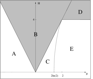
Figure 10: The phase diagramm of the $t$-$J$ model, shaded regions correspond to a ferromagnetic ground state.

In order to calculate the contributions of the impurity to the low–temperature specific heat we need to consider different characteristic regions (see Fig. 10) of the $t$-$J$ model as it was done for the Hubbard model by Takahashi [49]. As in [49] we assume $H\gg T$ so we can neglect the effects of the string solutions. (An alternative approach which overcomes this restriction has recently been used in [45] to compute bulk thermodynamic properties in the $t$-$J$ model).
Region A: The region is characterized by $\mu<-{H\over 2}$. For $T=0$ the electron density is zero as $A=B=\infty$. The low temperature free energy per site is given by

$$\frac{\Delta F_{\rm bulk}}{L}=\frac{F_{\rm bulk}-F_{\rm bulk}(T=0)}{L} = -T\int_{-\infty}^{\infty}d\lambda\ a_{2}(\lambda)\ln(1+e^{-\Psi\over T})-T\int_{-\infty}^{\infty}d\lambda\ a_{1}(\lambda)\ln(1+e^{-\varepsilon\over T})$$ (6.1)

$$\approx -{2T\over\pi}\int_{0}^{\infty}d\lambda\ {1\over\lambda^{2}}\ln(1+e^{2\mu\over T}e^{-2\over\lambda^{2}T})-{T\over\pi}\int_{0}^{\infty}d\lambda\ {1\over\lambda^{2}}\ln(1+e^{\mu+H/2\over T}e^{-1\over\lambda^{2}T})$$

$$\approx -{1\over\sqrt{2\pi}}T^{3/2}e^{2\mu\over T}-{1\over 2\sqrt{\pi}}T^{3/2}e^{\mu+H/2\over T}$$

The impurity contribution to the low temperature free energy is

$$\Delta F_{\alpha}=F_{\rm imp}-F_{\rm imp}(T=0)=-T\int_{-\infty}^{\infty}d\lambda\ a_{\alpha}(\lambda)\ln(1+e^{-\Psi\over T})\approx-{\alpha\over 2\sqrt{2\pi}}T^{3/2}e^{2\mu\over T}\ .$$ (6.2)

Region B: For $T=0$ this region, characterized by $-H/2<\mu<H/2$, is the ferromagnetic phase with electron density varrying as $0<n_{e}<1$. The right boundary line is defined by $B=\infty$ the left one by $A=B=\infty$. The low temperature free energies are given by

$$\frac{\Delta F_{\rm bulk}}{L}\approx-{\pi T^{2}\over 6}{1\over v_{s}}\qquad\Delta F_{\alpha}\approx-{\pi T^{2}\over 6}{f_{s}\over v_{s}}\ .$$ (6.3)

Region C: In this region, characterized by $0<A,B<\infty$, the electron density varries between $0<n_{e}<1$ at zero temperature. The right boundary line defined by $B=0$ can be calculated with aid of (4.12) for small magnetic field and with an iterative solution of (4.3) for $H\stackrel{{\scriptstyle<}}{{\sim}}4$. The low temperature free energies are given by

$$\frac{\Delta F_{\rm bulk}}{L}\approx-{\pi T^{2}\over 6}\left[{1\over v_{s}}+{1\over v_{c}}\right]\qquad\Delta F_{\alpha}\approx-{\pi T^{2}\over 6}\left[{f_{s}\over v_{s}}+{f_{c}\over v_{c}}\right]$$ (6.4)

Region D: This region is characterized by $\mu>H/2>2$. For $T=0$ we obtain the ferromagnetic half–filled band. The low temperature free energy is given by

$$\frac{\Delta F_{bulk}}{L}=-T\int_{-\infty}^{\infty}d\lambda\ a_{1}(\lambda)\ln(1+e^{-\varepsilon_{s}\over T})\approx-{4T\over\pi}\int_{0}^{\infty}d\lambda\ \ln(1+e^{4-H\over T}e^{-16\lambda^{2}\over T})\approx-{1\over 2\sqrt{\pi}}T^{3/2}e^{4-H\over T}\ .$$ (6.5)

The impurity contribution to the low temperature free energy is

$$\Delta F_{\alpha}=-T\int_{-\infty}^{\infty}d\lambda\ a_{\alpha}(\lambda)\ln(1+e^{-\varepsilon_{c}\over T})\approx-Te^{H/2-\mu\over T}\ .$$ (6.6)

Region E: For $T=0$ this region is half-filled and non ferromagnetic. The low temperature free energy of the bulk is given by

$$\frac{\Delta F_{bulk}}{L}\approx-{\pi T^{2}\over 6}{1\over v_{s}}$$ (6.7)

The impurity contribution in this region can not be calculated in closed form. In the two limiting cases $A\ll 1$ and $A\gg 1$ we obtain the following results

$$\Delta F_{\alpha}\approx-{2\over\alpha}T^{3/2}\left\{\begin{array}[]{ll}{1\over\sqrt{3\pi\zeta(3)/2-\pi^{3}a}}e^{2\ln(2)-\mu+2a\over T}&\hbox{for~{}}A\gg 1\\[8.0pt] \sqrt{3\over 8}{1\over(4-H)^{{3\over 4}}}e^{H/2-\mu+{2\over 3\pi}(4-H)^{3/2}\over T}&\hbox{for~{}}A\ll 1\end{array}\right.$$ (6.8)

Wilson ratio in Region C: The specific heat of the bulk and the impurity in region C are given by

$$C_{v,bulk}=\frac{\pi T}{3}\left(\frac{1}{v_{s}}+\frac{1}{v_{c}}\right)\qquad C_{v,\alpha}=\frac{\pi T}{3L}\left(\frac{f_{s}}{v_{s}}+\frac{f_{c}}{v_{c}}\right)$$ (6.9)

In deriving these results we assumed that $H\gg T$. Defining

$$R=\frac{\chi_{H,\alpha}/\chi_{H,bulk}}{C_{v,\alpha}/C_{v,bulk}}=\frac{\left[\left(\frac{Z_{cc}-2Z_{sc}}{Z_{cs}-2Z_{ss}}\right)^{2}\frac{f_{c}}{f_{s}}+\frac{v_{c}}{v_{s}}\right]\left[1+\frac{v_{c}}{v_{s}}\right]}{\left[\left(\frac{Z_{cc}-2Z_{sc}}{Z_{cs}-2Z_{ss}}\right)^{2}+\frac{v_{c}}{v_{s}}\right]\left[\frac{f_{c}}{f_{s}}+\frac{v_{c}}{v_{s}}\right]}.$$ (6.10)

and if we assume that the limits $T\rightarrow 0$ and $H\rightarrow 0$ commute we can calculate a “Wilson ratio”

$$R_{W}=\lim_{H\to 0}R=\frac{1+\frac{v_{c}}{v_{s}}}{\frac{f_{c}}{f_{s}}+\frac{v_{c}}{v_{s}}}\ .$$ (6.11)

Unlike for the case of the Kondo model (where spin and charge degrees of freedom decouple and the impurity couples only to the spin) there is no reason to expect $R_{W}$ to be universal for the present model.

From our analytical calculations we find for $B\ll 1$, $B\ll\alpha$ that $R_{W}=1-n_{e}\ll 1$. Near the empty band the ratio $R_{W}$ tends to one because $v_{c}$ approaches zero. Numerical calculations show that the limiting value one is most rapidly approached for small values of $\alpha$ (see Fig. 11). For comparison we quote the result for a Kondo impurity in a Luttinger liquid [12], for which $R_{W}=\frac{4}{3}(1+\frac{v_{s}}{v_{c}})$.

7 Transport Equations

Following Shastry and Sutherland [50] (see also [51]) we will now calculate spin- and charge stiffnesses from the finite-size corrections to the ground state energy of the model with twisted boundary conditions. For the $t$-$J$ model the bulk stiffnesses were determined in [43]. Our analysis follows closely the discussion given in [44]. Our goal is to evaluate the ground state energy as a function of the twist angles $\phi_{\uparrow}$ and $\phi_{\downarrow}$. Imposing twisted boundary conditions the BAE (3.3) are modified in the following way

$$\left(\frac{\lambda_{j}-{i\over 2}}{\lambda_{j}+{i\over 2}}\right)^{L}\left(\frac{\lambda_{j}-{\alpha+1\over 2}i}{\lambda_{j}+{\alpha+1\over 2}i}\right) = e^{-i\phi_{\uparrow}}\prod^{N_{\downarrow}}_{\gamma=1}\frac{\lambda_{j}-\lambda^{(1)}_{\gamma}-{i\over 2}}{\lambda_{j}-\lambda^{(1)}_{\gamma}+{i\over 2}}\ ,\quad j=1,\ldots,N_{e}\ ,$$

$$\prod^{N_{e}}_{j=1}\frac{\lambda^{(1)}_{\gamma}-\lambda_{j}+{i\over 2}}{\lambda^{(1)}_{\gamma}-\lambda_{j}-{i\over 2}} = -e^{i(\phi_{\uparrow}-\phi_{\downarrow})}\prod^{N_{\downarrow}}_{\beta=1}\frac{\lambda^{(1)}_{\gamma}-\lambda^{(1)}_{\beta}+i}{\lambda^{(1)}_{\gamma}-\lambda^{(1)}_{\beta}-i}\ ,\quad\gamma=1,\ldots,N_{\downarrow}\ .$$ (7.1)

For technical reasons it is convenient to use a different representation of the BAE first introduced by Sutherland for the $t$-$J$ model without impurity [29]. This can be obtained by a particle–hole transformation in the space of rapidities which is done in Appendix A. The final BAE are given by

$$\left(\frac{\lambda_{j}+{i\over 2}}{\lambda_{j}-{i\over 2}}\right)^{L} = -e^{i\phi_{s}}\prod^{M^{(1)}+N_{\downarrow}-1}_{k=1}\frac{\lambda_{j}-\lambda_{k}+i}{\lambda_{j}-\lambda_{k}-i}\ \prod^{M^{(1)}}_{\gamma=1}\frac{\lambda_{j}-\lambda_{\gamma}^{(1)}-{i\over 2}}{\lambda_{j}-\lambda_{\gamma}^{(1)}+{i\over 2}},\quad j=1,\ldots,L+1-N_{\uparrow}\ ,$$

$$\prod^{M^{(1)}+N_{\downarrow}-1}_{j=1}\frac{\lambda_{\gamma}^{(1)}-\lambda_{j}-{i\over 2}}{\lambda_{\gamma}^{(1)}-\lambda_{j}+{i\over 2}} = e^{-i\phi_{c}}\frac{\lambda_{\gamma}^{(1)}+i{\alpha\over 2}}{\lambda_{\gamma}^{(1)}-i{\alpha\over 2}}\quad\gamma=1,\ldots,M^{(1)}=L+2-N_{\uparrow}-N_{\downarrow}\ ,$$ (7.2)

where the twist–angles are given by $\phi_{s}=\phi_{\uparrow}-\phi_{\downarrow}$ and $\phi_{c}=\phi_{\downarrow}$ [44].

The equations (7.2) can be simplified by making use of the ‘string-hypothesis’, which states that for $L\rightarrow\infty$ all solutions are composed of real $\lambda^{(1)}_{\gamma}$’s whereas the $\lambda$’s are distributed in the complex plane according to the description

$$\lambda^{n,j}_{\beta}=\lambda^{n}_{\beta}+i\left(\frac{n+1}{2}-j\right)\ ,\quad j=1\ldots n\ ,$$ (7.3)

where $\beta=1\ldots M_{n}$ labels different ‘strings’ of length $n$ and $\lambda^{n}_{\beta}$ is real. The imaginary parts of the $\lambda$’s can now be eliminated from (7.2) via (7.3). Taking the logarithm of the resulting equations (for $M_{n}$ strings (7.3) of length $n$ and $M^{(1)}$ $\lambda^{(1)}$’s (note that $\sum_{n=1}^{\infty}nM_{n}=L+1-N_{\uparrow}$)) we arrive at

$$\frac{2\pi}{L}I^{n}_{\beta} = \theta(\frac{\lambda^{n}_{\beta}}{n})-\frac{1}{L}\sum_{(m\gamma)}\theta_{mn}(\lambda^{n}_{\beta}-\lambda^{m}_{\gamma})+\frac{1}{L}\sum_{\gamma=1}^{M^{(1)}}\theta(\frac{\lambda^{n}_{\beta}-\lambda^{(1)}_{\gamma}}{n})+\frac{\phi_{s}}{L},\beta=1\ldots M_{n}$$

$$\frac{2\pi}{L}J_{\gamma} = \frac{1}{L}\sum_{(n\beta)}\theta(\lambda^{(1)}_{\gamma}-\lambda^{n}_{\beta})+\frac{1}{L}\theta(\frac{\lambda^{(1)}_{\gamma}}{\alpha})+\frac{\phi_{c}}{L}\ ,\gamma=1\ldots M^{(1)}\ ,$$ (7.4)

where $I^{n}_{\beta}$ and $J_{\gamma}$ are integer or half-odd integer numbers, $\theta(x)=2\arctan(2x)$ and

$$\theta_{n,m}(x)=(1-\delta_{m,n})\theta({x\over{|n-m|}})+2\ \theta({x\over{|n-m|+2}})+\dots+2\ \theta({x\over{n+m-2}})+\theta({x\over{n+m}})\ .$$ (7.5)

For vanishing twist angles the ranges of the “quantum numbers” $I^{n}_{\beta}$ and $J_{\gamma}$ are given by

$$|I^{n}_{\beta}| \leq \frac{1}{2}(L+M^{(1)}+M_{n}-2\sum_{m=1}^{\infty}{\rm min}\{m,n\}M_{m}-1)\ ,$$

$$|J_{\gamma}| \leq \frac{1}{2}(\sum_{n=1}^{\infty}M_{n}-1)\ .$$ (7.6)

Ground state and excitations can now be constructed by specifying sets of integer (half-odd integer) numbers $I^{n}_{\beta}$ and $J_{\gamma}$ and turning equations (7.4) into sets of coupled integral equations in the thermodynamic limit. The antiferromagnetic ground state for zero twist angles is obtained by filling consecutive quantum numbers $I^{1}_{\beta}$ and $J_{\gamma}$ symmetrically around zero, which corresponds to filling two Fermi seas of spin and charge degrees of freedom respectively. The effect of an infinitesimally small flux is to shift the distribution of roots (i.e. the rapidities in the Fermi seas) by a constant amount. This shift leads to a twist-angle dependent contribution to the ground state energy. The ground state (in the presence of flux) is described in terms of the root densities $\rho_{\alpha}(\lambda)$, which are solutions of the integral equations

$$\rho_{s}(\lambda) = a_{1}(\lambda)-\int_{\tilde{\Lambda}_{s}^{-}}^{\tilde{\Lambda}_{s}^{+}}d\mu\ a_{2}(\lambda-\mu)\ \rho_{s}(\mu)+\int_{\tilde{\Lambda}_{c}^{-}}^{\tilde{\Lambda}_{c}^{+}}d\mu\ a_{1}(\lambda-\mu)\ \rho_{c}(\mu)+{\cal O}(L^{-2})$$

$$\rho_{c}(\mu) = \int_{\tilde{\Lambda}_{s}^{-}}^{\tilde{\Lambda}_{s}^{+}}d\mu^{\prime}\ a_{1}(\mu-\mu^{\prime})\ \rho_{s}(\mu^{\prime})\ +\frac{a_{\alpha}(\mu)}{L}+{\cal O}(L^{-2}).$$ (7.7)

Here $\tilde{\Lambda}_{\beta}^{\pm}$ are the Fermi points for the finite system in the presence of the flux. We denote the Fermi points for the infinite system without flux by $\pm\Lambda_{\beta,0}$ (note that the distribution of roots is symmetric around zero in that case). For further convenience we define the quantities

$$D_{\beta}=-\frac{1}{2}\int_{\tilde{\Lambda}_{\beta}^{+}}^{\infty}\!\!\!\!\!\!-\!\!\!\int_{-\infty}^{\tilde{\Lambda}_{\beta}^{-}}d\mu\ \rho_{\beta}(\mu)\ .$$ (7.8)

In order to evaluate the stiffnesses we need to consider infinitesimal flux only, which yields a correction of order $\frac{1}{L}$ to the ground state energy. Following through the standard steps [47, 52] and taking into account the $\frac{1}{L}$-corrections from the infinitesimal flux we obtain

$$E(\phi_{s},\phi_{c},\alpha)=Le(\Lambda_{\beta,0})+f(\Lambda_{\beta,0})-\frac{\pi}{6L}(v_{s}+v_{c})+2\pi LD^{T}{\bf Z}{\bf V}{\bf Z}^{T}D+o(\frac{1}{L}),$$ (7.9)

where ${\bf Z}$ is the dressed charge matrix (4.30), $D=(D_{c},D_{s})^{\top}$ and $V={\rm diag}(v_{c},v_{s})$. Here $e(\Lambda_{\beta,0})$ and $f(\Lambda_{\beta,0})$ are the ground state energy per site and impurity energy in the infinite system without flux. The quantity $D_{\beta}$ is given by

$$D_{\beta}=\frac{\phi_{\beta}}{2\pi L}\ .$$ (7.10)

In order to study the charge and spin conductivities and the respective currents we consider the energy-difference $\Delta E=E(\phi_{s},\phi_{c},\alpha)-E(0,0,\alpha)$. It can be cast in the form

$$\Delta E={1\over L}\phi_{\alpha}D_{\alpha\beta}\phi_{\beta}\ +\ {\rm subleading\ terms}.$$ (7.11)

According to [50] the charge (spin) stiffness $D^{(\rho)}$ ($D^{(\sigma)}$) is defined as

$$D^{(\rho)}={L\over 2}{\partial^{2}\over\partial\phi^{2}}\Delta E(\phi_{c}=\phi,\phi_{s}=0,\alpha)\ ,\quad D^{(\sigma)}={L\over 2}{\partial^{2}\over\partial\phi^{2}}\Delta E(\phi_{c}=\phi,\phi_{s}=-2\phi,\alpha).$$ (7.12)

Using the expressions (7.10) in (7.9) and (7.12) we find that the stiffnesses are not modified by the impurity to leading order in $\frac{1}{L}$. It is clear from the above analysis that there are corrections due to the impurity in the subleading terms. The precise form of these expressions is not of particular interest from a physical point of view and as the extension of the above finite-size analysis to the subleading orders is rather difficult we refrain from determining them. The important point is that despite the presence of the impurity the stiffnesses are still finite and the dc-conductivity is thus infinite. We believe that this fact is due to the integrability and the related absence of backscattering.

This means that the integrable impurity considered here is of a completely different nature than the “weak link”-type potential impurity considered in [1, 2, 3, 8]: as the electron-electron interactions are repulsive in the supersymmetric $t$-$J$ model a weak link drives the system to a strong coupling fixed point characterized by the vanishing of the conductivity.

7.1 Stiffnesses for finite density of impurities

Let us now turn to transport properties for the system with a finite density of impurities. The necessary steps are the same as above, the main difference being the change of integral equations describing the ground state from (7.7) to

$$\rho_{s}(\lambda) = (1-n_{i})a_{1}(\lambda)-\int_{\tilde{\Lambda}_{s}^{-}}^{\tilde{\Lambda}_{s}^{+}}d\mu\ a_{2}(\lambda-\mu)\ \rho_{s}(\mu)+\int_{\tilde{\Lambda}_{c}^{-}}^{\tilde{\Lambda}_{c}^{+}}d\mu\ a_{1}(\lambda-\mu)\ \rho_{c}(\mu)\ ,$$

$$\rho_{c}(\mu) = n_{i}a_{\alpha}(\mu)+\int_{\tilde{\Lambda}_{s}^{-}}^{\tilde{\Lambda}_{s}^{+}}d\mu^{\prime}\ a_{1}(\mu-\mu^{\prime})\ \rho_{s}(\mu^{\prime})\ ,$$ (7.13)

where $n_{i}$ is the concentration of impurities. As the integral equations for the dressed energies remain unchanged, the dressed charge is not modified and $A(\mu,H)$ and $B(\mu,H)$ are not changed. However, the presence of a finite density of impurities leads to changes in the electron density, which is now given by $n_{e}=(1-n_{i})D_{bulk}+n_{i}N_{\alpha}$ and the Fermi velocities, which are found to be of the form

$$\tilde{v}_{\beta}=\frac{v_{\beta}}{1+n_{i}(f_{\beta}-1)}\ .$$ (7.14)

Here $v_{\beta}$ are the velocities of the normal $t$-$J$-chain and the $f_{\beta}$ are defined in (4.28). From (7.12) the following form of the stiffnesses is easily deduced

$$D^{(\rho)}={1\over 2\pi}\left(\tilde{v}_{c}Z^{2}_{cc}+\tilde{v}_{s}Z^{2}_{cs}\right),\qquad D^{(\sigma)}={1\over 2\pi}\left(\tilde{v}_{c}(Z_{cc}-2Z_{sc})^{2}+\tilde{v}_{s}(Z_{cs}-2Z_{ss})^{2}\right).$$ (7.15)

Using the results of the above sections we can evaluate these expressions analytically for small magnetic field close to “maximal filling” ($t$-$J$ sites singly occupied, impurities doubly occupied) and near the critical electron density $n_{c}$. This is done in the following two subsections. Finally we present numerical results for the general case.

7.1.1 Stiffnesses for small magnetic field near maximal filling

Close to maximal filling and for $\alpha\gg B$ the leading term of the charge stiffness is found to be

$$D^{(\rho)}\approx{1\over 2\pi}\tilde{v}_{c}Z^{2}_{cc}=\frac{3\zeta(3)}{4\pi\ln(2)}\frac{B}{1+n_{i}\left(\frac{2}{\ln(2)\alpha}+\frac{2a}{\ln^{2}(2)\alpha}-1\right)}+\ldots$$ (7.16)

Combining (7.16) with the result for the electron density we obtain the following limiting value for the slope of the charge stiffness as a function of density

$${\partial D^{(\rho)}\over\partial n_{e}}|_{n_{e}=1+n_{i}}=-{3\zeta(3)\over 8\ln^{2}(2)}{1\over\left[1+n_{i}\left(\frac{2}{\ln(2)\alpha}+\frac{2a}{\ln^{2}(2)\alpha}-1\right)\right]^{2}}+\ldots$$ (7.17)

In the strong-coupling limit this turns into

$$\lim_{\alpha\to\infty}{\partial D^{(\rho)}\over\partial n_{e}}|_{n_{e}=1+n_{i}}=-{3\zeta(3)\over 8\ln^{2}(2)}{1\over\left(1-n_{i}\right)^{2}}={1\over\left(1-n_{i}\right)^{2}}{\partial D^{(\rho)}_{tJ}\over\partial n_{e}}|_{n_{e}=1}$$ (7.18)

The leading term of the spin stiffness for $B\ll 1$ and $\alpha\gg B$ is given by

$$D^{(\sigma)}\approx{1\over 2\pi}\tilde{v}_{s}\left(Z_{cs}-2Z_{ss}\right)^{2}={v_{s}\over\pi}\left(1-{1\over 4\ln(H/H_{0})}\right)^{2}{1\over 1+n_{i}(f_{s}-1)}\ .$$ (7.19)

In the limit $\alpha\to\infty$ we find

$${\partial D^{(\sigma)}\over\partial n_{e}}|_{n_{e}=1+n_{i}}=\pi\left(1-{1\over 2\ln(H/H_{0})}\right){1\over(1-n_{i})^{2}}={1\over\left(1-n_{i}\right)^{2}}{\partial D^{(\sigma)}_{tJ}\over\partial n_{e}}|_{n_{e}=1}\ .$$ (7.20)

7.1.2 Stiffnesses slightly above $n_{c}$

As pointed out above it is possible to derive analytic expressions for the stiffnesses for densities slightly above $n_{c}$. However the resulting expressions are found to be rather complicated so that we refrain from listing them here.

The derivative of the spin–stiffness with respect to the electron density at $n_{e}=n_{c}^{+}$ is always positive, taking its maximum at $\alpha=0$ and its minimum $0$ in the limit $\alpha\to\infty$.

The derivative of the charge–stiffness with respect to the electron density at $n_{e}=n_{c}^{+}$ changes sign as a function of $\alpha$ (see Fig. 12).

7.1.3 Numerical Results

The results for the charge stiffness in systems with impurity densities $n_{i}=0.2$ and two different values of the bulk field $H$ are depicted in Fig. 13 and Fig. 14. The charge stiffness for $n_{i}=0.5$ is shown in Fig. 15. For comparison we plot the result for the charge–stiffness $D^{\rho}_{tJ}$ for the $t$-$J$ model without impurities as calculated in [44]. We note that the maximal allowed band-filling is larger than one as the impurity sites can be doubly occupied. We see that for small band-fillings above the critical density the charge-stiffness is reduced as compared to the pure $t$-$J$ case. For larger band fillings the stiffness is found to increase in the presence of impurities. This is easily understood: due to the constraint of single occupancy the stiffness vanishes as we approach half-filling in the $t$-$J$ chain. The impurity sites can be doubly occupied, which gives the electrons “space to move” and leads to an increase in the stiffness. For large fillings the stiffness increases with increasing $\alpha$ because (as can be deduced from the $a\rightarrow\infty$ limit) the impurity sites become (on average) closer and closer to being doubly occupied, which again makes it easier for the electrons to move along the $t$-$J$ sites. Last but not least let us discuss the limiting case $\alpha=\infty$ at impurity density $n_{i}$, i.e. there are $Ln_{i}$ impurity sites and $L(1-n_{i})$ $t$-$J$ sites. For electron densities $n_{e}$ smaller than $n_{i}$ the (spin-up) electrons (in the ground state) occupy only impurity sites which do not interact with the $t$-$J$ sites. Thus the stiffness is identically zero. For electron densities $n_{i}<n_{e}<n_{i}+(1-n_{i})n_{c}$ the saturated ferromagnetic ground state on the $t$-$J$ sites is formed whereas all impurity sites are singly occupied. The stiffness is completely determined by the $t$-$J$ sites. For densities in the interval $n_{i}+(1-n_{i})n_{c}<n_{e}<2n_{i}+(1-n_{i})n_{c}$ the impurity sites become doubly occupied and the stiffness does not change. For $n_{e}>2n_{i}+(1-n_{i})n_{c}$ all impurity sites are doubly occupied and the stiffness follows (up to a rescaling by $\frac{1}{1-n_{i}}$) the $t$-$J$ curve above the critical density $n_{c}$ (see (7.20) and (7.18)).

The spin-stiffness for impurity density $0.2$ is shown in Fig. 16. We see that the stiffness is decreased at low fillings (this decrease is more pronounced for larger values of $\alpha$) and approaches the “pure” $t$-$J$ value for large fillings. The behaviour in the limit $\alpha\to\infty$ is the same as for the charge stiffness.

8 Impurity Phase-Shifts

In this section we evaluate the phase shifts acquired by the elementary excitations, holons and spinons, when scattering off the impurity. The results give a good measure of the effects of the impurity on excited states. In particular we can infer from the phase-shifts how the impurity couples to spin and charge degrees of freedom. We start by briefly reviewing some important facts about the low-lying excitations in the $t$-$J$ model [31]. The elementary excitations are collective modes of spin or charge degrees of freedom. The spin excitations are called spinons and carry spin $\pm\frac{1}{2}$ and zero electric charge. They are very similar to the spin-waves in the Heisenberg XXX chain. The charge excitations are called holons and antiholons, carry zero spin and charge $\mp e$. Thus holons correspond to physical holes. At half-filling only holons can be excited as the charge Fermi sea is completely empty. The excitation energies are given by $\varepsilon_{c,s}$ defined in (4.3). The respective physical momenta are given in terms of the solutions of the following set of coupled integral equations

$${\tt p}_{s}(\lambda) = -\theta(\lambda)-\int_{-A}^{A}d\nu\ a_{2}(\lambda-\nu){\tt p}_{s}(\nu)+\int_{-B}^{B}d\nu\ a_{1}(\lambda-\nu)\ {\tt p}_{c}(\nu)\ ,$$

$${\tt p}_{c}(\lambda) = \int_{-A}^{A}d\nu\ a_{1}(\lambda-\nu)\ {\tt p}_{s}(\nu).$$ (8.1)

The mometum of e.g. a holon-antiholon excitation is given by $P_{c{\bar{c}}}={\tt p}_{c}(\Lambda^{p})-{\tt p}_{c}(\Lambda^{h})$ where $\Lambda^{p}$ and $\Lambda^{h}$ are the spectral parameters of the holon and antiholon respectively. We thus would define the physical holon momentum as $p_{c}(\Lambda^{p})={\tt p}_{c}(\Lambda^{p})-{\tt p}_{c}(B)$. At half-filling the spinon ($p_{s}$) and holon ($p_{c}$) momenta are given by

$$p_{s}(\lambda) = 2\arctan(\exp(\pi\lambda))-\pi\ ,$$

$$p_{c}(\lambda) = \frac{\pi}{2}+i\ \ln\left(\frac{\Gamma(\frac{1-i\lambda}{2})}{\Gamma(\frac{1+i\lambda}{2})}\frac{\Gamma(1+\frac{i\lambda}{2})}{\Gamma(1-\frac{i\lambda}{2})}\right).$$ (8.2)

The scattering matrix has been determined by means of Korepin’s method [39, 53] in [31]. At half-filling the spinon-spinon S-matrix $S(\lambda)$, the spinon-holon ($sc$) and holon-holon ($cc$) scattering phases are given by

$$S(\lambda) = i\frac{\Gamma(\frac{1-i\lambda}{2})}{\Gamma(\frac{1+i\lambda}{2})}\frac{\Gamma(1+\frac{i\lambda}{2})}{\Gamma(1-\frac{i\lambda}{2})}\left(\frac{\lambda}{\lambda-i}I-\frac{i}{\lambda-i}P\right)\ ,$$

$$\exp(i\varphi_{sc}(\lambda)) = -i\frac{1+ie^{\pi\lambda}}{1-ie^{\pi\lambda}}\ ,\qquad\exp(i\varphi_{cc}(\lambda))=\frac{\Gamma(\frac{1+i\lambda}{2})}{\Gamma(\frac{1-i\lambda}{2})}\frac{\Gamma(1-\frac{i\lambda}{2})}{\Gamma(1+\frac{i\lambda}{2})}$$ (8.3)

where $I$ and $P$ are the $4\times 4$ identity and permutation matrices respectively. Below half-filling the S-matrices are given in terms of the solution of integral equations.

The impurity phase-shifts can be computed by the standard method of Korepin [53], Andrei et. al. [54, 55]. In the most general case of a bulk magnetic field and arbitrary filling factor the phase-shifts can be expressed only in terms of the solution of a set of coupled integral equations, the analysis of which is rather difficult. We therefore constrain ourselves to the case of a microscopic number of holes in the half-filled ground state in the absence of a bulk magnetic field.

The basic ingredient for computing impurity phase-shifts is the quantization condition for factorized scattering of two particles with rapidities $\lambda_{1,2}$ on a ring of length $N$ (including the impurity site)

$$\exp(iNp(\lambda_{1}))S(\lambda_{1}-\lambda_{2})e^{i\psi(\lambda_{1})}=1\ ,$$ (8.4)

where $p(\lambda)$ is the expression for the physical momentum of the corresponding (infinite) periodic system, $S(\lambda)$ are the bulk scattering matrices for scattering of particles $1$ and $2$, and $\psi(\lambda_{1})$ is the phase-shift acquired by particle $1$ when scattering off the impurity. We note that the condition (8.4) incorporates the fact that there is no backscattering at the impurity. For the present model the absence of backscattering follows from the conservation laws for the rapidities: although momentum is not a good quantum number for the ring with impurity, excited states can still be characterized by the rapidity variables (see below for an example). We would expect that if the impurity contained a backscattering term mixing of states with different rapidities would occur. This is not the case in the present model which indicates the absence of backscattering. We note that the absence of backscattering on the level of the “bare” Bethe Ansatz equations (3.3) (which describe the scattering of excitations over the empty ground state) is not sufficient to deduce the absence of backscattering over the antiferromagnetic ground state because the impurity gets dressed by the holons and spinons in the ground state Fermi seas, and the two-particle scattering processes between holons and spinons do contain backscattering terms. Therefore the treatment of [56] does not apply in the present case.

In what follows we will extract the holon and spinon impurity phase-shifts from the spinon-holon scattering state, for which the condition (8.4) turns into scalar equations for the scattering phases, which after taking the logarithm read

$$Np_{s}(\lambda^{h})+\varphi_{sc}(\lambda^{h}-\Lambda^{p})+\psi_{s}(\lambda^{h})=0\ {\rm mod}\ 2\pi\ ,$$

$$Np_{c}(\Lambda^{p})+\varphi_{sc}(\Lambda^{p}-\lambda^{h})+\psi_{c}(\Lambda^{p})=0\ {\rm mod}\ 2\pi\ .$$ (8.5)

Here $\lambda^{h}$ and $\Lambda^{p}$ are the rapidities of the spinon and holon respectively. Comparing these conditions with certain quantities (“counting functions”) that can be calculated from the Bethe Ansatz solution one can then read off the boundary phase-shifts $\psi_{s,c}$.

Let us start by constructing the half-filled antiferromagnetic ground state for even length $L$ of the host chain, where we furthermore assume that $\frac{L}{2}$ is even as well. The ground state is obtained by choosing $M_{1}=\frac{L}{2}$, $M^{(1)}=0$ in (7.4) and filling the half-odd integers $I^{1}_{\beta}$ symmetrically around zero. In the thermodynamic limit this corresponds to filling a Fermi sea of rapidities $\lambda^{1}_{\beta}$ between $-\infty$ and $\infty$, where the root density $\rho_{s}(\lambda^{1}_{\beta})=\lim_{L\to\infty}\frac{1}{(L+1)(\lambda^{1}_{\beta+1}-\lambda^{1}_{\beta})}$ is given in terms of the integral equation

$$\rho_{s}(\lambda)=a_{1}(\lambda)\left(1-\frac{1}{L+1}\right)-\int_{-\infty}^{\infty}d\nu\ a_{2}(\lambda-\nu)\ \rho_{s}(\nu)\ .$$ (8.6)

The spinon-holon scattering state characterized by choosing $M_{1}=\frac{L}{2},M^{(1)}=1$ in the Bethe equations (7.4). There are $\frac{L}{2}+1$ vacancies for the integers $I^{1}_{\alpha}$ and thus one hole in the Fermi sea of $\lambda^{1}_{\beta}$. We denote the rapidity corresponding to this hole by $\lambda^{h}$. The rapidity corresponding to the holon is denoted by $\Lambda^{p}$. The Bethe equations read

$$\frac{2\pi}{L+1}I_{\beta} = (1-\frac{1}{L+1})\theta(\lambda_{\beta})-\frac{1}{L+1}\sum_{\beta^{\prime}=1}^{\frac{L}{2}+1}\theta(\frac{\lambda_{\beta}-\lambda_{\beta^{\prime}}}{2})+\frac{1}{L+1}\left[\theta(\frac{\lambda_{\beta}-\lambda^{h}}{2})+\theta(\lambda_{\beta}-\Lambda^{p})\right],$$

$$\frac{2\pi}{L+1}J = \frac{1}{L+1}\sum_{\beta=1}^{\frac{L}{2}+1}\theta(\Lambda^{p}-\lambda_{\beta})+\frac{1}{L+1}\theta(\frac{\Lambda^{p}}{\alpha})-\frac{1}{L+1}\theta(\Lambda^{p}-\lambda^{h}),$$ (8.7)

where $J$ is a half-odd integer number. In the limit $L\rightarrow\infty$ the distribution of roots $\lambda_{\beta}$ is described by a single integral equation for the density of roots $\rho_{s}(\lambda)$, which is of Wiener-Hopf form but cannot be solved in a form sufficiently explicit for the purpose of determining the impurity phase-shifts. The main complication is that we need to take into account all contributions of order $\frac{1}{L+1}$ and thus must deal with the fact that the roots are distributed not between $-\infty$ and $\infty$ but between two finite, $L$-dependent values $-A$ and $A$. It can however be checked numerically that making the assumption that the contributions due to the shift of integration boundaries will be of higher order in $\frac{1}{L+1}$ as far as the impurity phase-shifts are concerned (and thus taking $A=\infty$) yields the correct result. The integral equation then can be solved by Fourier transform

$$\widetilde{\rho_{s}}(\omega)=\widetilde{G}_{0}(\omega)+\frac{1}{L+1}\left\{\widetilde{G}_{1}(\omega)e^{i\omega\lambda^{h}}-\widetilde{G}_{0}(\omega)[1-2e^{i\omega\Lambda^{p}}\right\},$$ (8.8)

where $\widetilde{\rho_{s}}(\omega)$ is the Fourier transform of $\rho_{s}(\omega)$ and where $\widetilde{G}_{x}(\omega)=\frac{\exp(-\frac{x}{2}|\omega|)}{2\cosh(\frac{\omega}{2})}$.

For the further analysis it is convenient to define counting functions $z_{s}(\lambda)$ and $z_{c}(\lambda)$

$$z_{s}(\lambda) = \frac{L}{2\pi}\theta(\lambda)-\frac{1}{2\pi}\sum_{\beta=1}^{\frac{L}{2}+1}\theta(\frac{\lambda-\lambda_{\beta}}{2})+\frac{1}{2\pi}\left[\theta(\frac{\lambda-\lambda^{h}}{2})+\theta(\lambda-\Lambda^{p})\right],$$

$$z_{c}(\Lambda) = \frac{1}{2\pi}\sum_{\beta=1}^{\frac{L}{2}+1}\theta(\Lambda-\lambda_{\beta})-\frac{1}{2\pi}\left[\theta(\Lambda-\lambda^{h})+\theta(\frac{\Lambda}{\alpha})\right].$$ (8.9)

Note that for any root e.g. $\lambda_{\alpha}$ of (8.7) the counting function takes the integer value $z_{s}(\lambda_{\alpha})=I_{\alpha}$ by construction. In the thermodynamic limit $\frac{1}{L+1}$ times the derivative of $z_{s}$ yields the distribution function of rapidities $\rho_{s}(\lambda)$. Straightforward integration of the density $\rho_{s}(\lambda)$ yields the following results for the counting functions in the thermodynamic limit evaluated at the rapidities of the spinon and holon respectively

$$2\pi z_{s}(\lambda^{h}) = (L+1)p_{s}(\lambda^{h})+\varphi_{sc}(\lambda^{h}-\Lambda^{p})+\phi_{s}(\lambda^{h})=0\ {\rm mod}\ 2\pi\ ,$$

$$-2\pi z_{c}(\Lambda^{p}) = (L+1)p_{c}(\Lambda^{p})+\varphi_{sc}(\Lambda^{p}-\lambda^{h})+\phi_{c}(\Lambda^{p})=\pi\ {\rm mod}\ 2\pi\ ,$$ (8.10)

where $p_{s,c}(\lambda)$ are the spinon/holon momenta (8.2), $\varphi_{sc}(\lambda)$ is the bulk phase-shift for spinon-holon scattering (8.3), and

$$\phi_{s}(\lambda)=-p_{s}(\lambda)\ ,\qquad\phi_{c}(\lambda)=-p_{c}(\lambda)+\pi-\theta(\frac{\lambda}{\alpha})\ .$$ (8.11)

From these equations we can now infer the boundary phase shifts by comparing them with the quantization condition (8.5), which yields

$$e^{i\psi_{s}(\lambda)} = C\ \frac{\Gamma(\frac{1}{4}+\frac{i\lambda}{2})}{\Gamma(\frac{1}{4}-\frac{i\lambda}{2})}\frac{\Gamma(\frac{3}{4}-\frac{i\lambda}{2})}{\Gamma(\frac{3}{4}+\frac{i\lambda}{2})}\ ,$$

$$e^{i\psi_{c}(\lambda)} = -C^{-1}\ \frac{\alpha-2i\lambda}{\alpha+2i\lambda}\ \frac{\Gamma(\frac{1}{2}-\frac{i\lambda}{2})}{\Gamma(\frac{1}{2}+\frac{i\lambda}{2})}\frac{\Gamma(1+\frac{i\lambda}{2})}{\Gamma(1-\frac{i\lambda}{2})},$$ (8.12)

where $C$ is an overall constant factor of unit modulus that cannot be determined within the Bethe Ansatz framework. Setting $C=-i$ we find that

$$e^{i\psi_{s}(\lambda)}=e^{-ip_{s}(\lambda)}\ ,\qquad e^{i\psi_{c}(\lambda)}=-\frac{\alpha-2i\lambda}{\alpha+2i\lambda}\ e^{-ip_{c}(\lambda)}\ ,$$ (8.13)

where $p_{s}$ and $p_{c}$ are the spinon and holon momenta at half-filling respectively. This result is interpreted in the following way: for the half-filled band doped with a finite number of holes the impurity site essentially decouples from the host chain in the sense that spinons and holons bypass it, which effectively shortens the lattice by one site (see Fig. 4)!
For the spinons this is the complete picture, whereas the holons still acquire a phase shift due to the fact that the impurity site is charged (recall that it is on average almost doubly occupied) and therefore interacts with the holons passing it by. The holon scattering phase has a pole at $\lambda=i\frac{\alpha}{2}$, which for $-2\leq\alpha\leq-1$ lies on the physical sheet and therefore corresponds to an impurity bound state. The restriction $\alpha<-1$ is imposed in order to have a hermitean hamiltonian [36]. The impurity therefore has the interesting property to lead to a holon bound state for sufficiently small negative $\alpha$ at half-filling.

9 Conclusion

In this paper we have studied the effects of an integrable impurity in a periodic $t$-$J$ model. The impurity couples to both spin and charge degrees of freedom and the coupling strength $\alpha$ can be varied continuously without losing integrability. The two limiting cases $\alpha=0$ and $\alpha=\infty$ have been shown to be described by effective (ground state) hamiltonians of a $t$-$J$ model with one extra site, and a decoupled impurity in a $t$-$J$ chain with twisted boundary conditions.

At zero temperature we have calculated the impurity magnetization and particle number for arbitrary band filling and bulk magnetic field. The impurity susceptibilities have been shown to exhibit the same types of singularities as the corresponding bulk susceptibilities. Similarly the low-temperature specific heat of impurity and bulk have the same temperature dependence. Transport properties have been determined through the calculation of spin and charge stiffnesses and finally the impurity phase shifts have been calculated for the half-filled band.

The supersymmetric $t$-$J$ model belongs to the class of Luttinger liquids with repulsive electron-electron interactions. The effects of potential impurities of the “weak-link” type were first investigated in [1, 2]. It was found that the system flows to a strong-coupling fixed point characterized by the vanishing of the dc conductivity. The physics of the impurity studied here is quite different: the dc-conductivity is unchanged by the presence of a single impurity.

As argued above the type of impurity considered here does not seem to contain backscattering terms on the level of the dressed excitations (holons and spinons). It would be interesting to verify this assertion by explicitly constructing the continuum limit of the model. However, due to the complicated structure of the impurity hamiltonian this is a difficult undertaking. The argument given above suggest that it is impossible to construct an impurity model containing backscattering off the impurity by means of the Quantum Inverse Scattering Method through the standard intertwining relation “$RTT=TTR$”: the rapidities of the elementary excitations will always be conserved quantities and are not affected by the scattering off the impurity. Clearly “generic” impurities ought to contain backscattering as only special potentials are reflectionless. From that point of view the integrable impurity considered in the present work is very special. The situation is similar to the (multichannel) Kondo model (viewed as a $1-d$ system). One may speculate that like for the case of a Kondo-impurity in a Luttinger liquid a backscattering term will drive the system to a new fixed point [12] so that the integrable impurity would represent an unstable fixed point in the sense of the renormalisation group. This is known to be the case for the spin system of Andrei and Johannesson [57]. As we have seen the integrable impurity nevertheless leads to interesting physical consequences.

Acknowledgements

We are grateful to A. Tsvelik and A.Jerez for important discussions and suggestions. F.H.L.E. is supported by the EU under Human Capital and Mobility fellowship grant ERBCHBGCT940709. He thanks the ITP at Hannover, where part of this work was performed, for hospitality. This work has been supported in part by the Deutsche Forschungsgemeinschaft under Grant No. Fr 737/2–1.

Appendix A Transformation of the BAE

To show the equivalence of the two sets of BAE (7.1) and (7.2) we use a method due to Woynarovich [58] and Bares et al[44]. We express the second set of (7.2) as a polynomial of degree $M^{(1)}+N_{\downarrow}$

$$P(w)=\prod_{j=1}^{M^{(1)}+N_{\downarrow}-1}(w-\lambda_{j}-{i\over 2})(w-i{\alpha\over 2})-e^{-i\phi_{c}}\prod_{\beta=1}^{M^{(1)}+N_{\downarrow}-1}(w-\lambda_{j}+{i\over 2})(w+i{\alpha\over 2})=0$$ (A.1)

and identify the first $M^{(1)}$ roots of (A.1) $w_{1},\ldots,w_{M^{(1)}}$ with $\lambda_{1}^{(1)},\ldots,\lambda_{M^{(1)}}^{(1)}$. Using the residue theorem we obtain the following equality:

$$\sum_{j=1}^{M^{(1)}}{1\over i}\ln\left[\frac{\lambda_{l}-\lambda_{j}^{(1)}+{i\over 2}}{\lambda_{l}-\lambda_{j}^{(1)}-{i\over 2}}\right]=\sum_{j=1}^{M^{(1)}}{1\over 2\pi i}\oint_{{\cal C}_{j}}dz{1\over i}\ln\left[\frac{\lambda_{l}-z+{i\over 2}}{\lambda_{l}-z-{i\over 2}}\right]\frac{d}{dz}\ln(P(z))$$ (A.2)

where ${\cal C}_{j}$ is a small contour including $\lambda_{j}^{(1)}$. Deforming the contour and denoting the $N_{\downarrow}$ other roots of (A.1) with $w^{\prime}_{1},\ldots,w^{\prime}_{N_{\downarrow}}$ we arrive at the following equality

$$\sum_{j=1}^{M^{(1)}}{1\over i}\ln\left[\frac{\lambda_{l}-\lambda_{j}^{(1)}+{i\over 2}}{\lambda_{l}-\lambda_{j}^{(1)}-{i\over 2}}\right]=-\sum_{j=1}^{N_{\downarrow}}{1\over i}\ln\left[\frac{\lambda_{l}-w^{\prime}_{j}+{i\over 2}}{\lambda_{l}-w^{\prime}_{j}-{i\over 2}}\right]+{1\over i}\ln\left[\frac{P(z_{n})}{P(z_{p})}\right],$$ (A.3)

where the last term comes from integration aorund the branch cut extending from $z_{n}=\lambda_{l}+i/2$ to $z_{p}=\lambda_{l}-i/2$. Using the form of $P(w)$ and substituting (A.3) into the first equation of (7.2) we obtain the first equation of (7.1) with the according twist–angle

$$\left(\frac{\lambda_{j}-{i\over 2}}{\lambda_{j}+{i\over 2}}\right)^{L}\left(\frac{\lambda_{j}-{\alpha+1\over 2}i}{\lambda_{j}+{\alpha+1\over 2}i}\right)=e^{-i(\phi_{c}+\phi_{s})}\prod^{N_{\downarrow}}_{\alpha=1}\frac{\lambda_{j}-\lambda^{(1)}_{\alpha}-{i\over 2}}{\lambda_{j}-\lambda^{(1)}_{\alpha}+{i\over 2}}\ ,\quad j=1,\ldots,N_{e}\ ,$$ (A.4)

The second equation of (7.1) can be obtained by the same steps starting with the first equation of (7.2). The twist–angles are related by $\phi_{s}=\phi_{\uparrow}-\phi_{\downarrow}$ and $\phi_{c}=\phi_{\downarrow}$ [44]. In [32, 33] it was shown that the BAE (7.2) for the $t$-$J$ model without impurity can be obtained by means of the QISM starting with a fermionic vacuum with all spins up. The corresponding vacuum state of the impurity model is given by a bosonic doubly occupied impurity site and all other sites occupied with spin up electrons. The algebraic Bethe–Ansatz starting from this vacuum can also be constructed.

Appendix B The three site model

The Bethe ansatz states do not form the complete set of eigenstates of the system but are the highest-weight states of the $gl(2|1)$ superalgebra (taking the Lai solutions of the BAE). Complementing the Bethe ansatz states with those obtained by the action of the $gl(2|1)$ lowering operators one obtains additional eigenstates. The completeness of this extended Bethe ansatz has been proven for some models as the spin-${1\over 2}$ Heisenberg chain, the supersymmetric $t$-$J$ model and the Hubbard model [33, 59, 60]. In this appendix we present a completeness analysis for impurity system considered here on a chain with three sites. This nontrivial example shows that the picture of [33, 59, 60] seems to hold in the present model as well. A detailed analysis of the general case is outside the scope of the present paper.

We need to consider the action (on states given by the Bethe Ansatz) of the spin lowering operator $S^{-}=\sum_{i=1}^{L+1}X_{i}^{\downarrow\uparrow}$ and the supersymmetry operators $Q_{\sigma}^{\dagger}$ ($Q_{\sigma}$ in the Sutherland case), which are given by

$$Q_{\downarrow}=\sum_{i=1,i\neq 2}^{L+1}X_{i}^{0\downarrow}+\sqrt{\alpha+1}X_{2}^{0\downarrow}+\sqrt{\alpha}X_{2}^{\uparrow 2}\ ,\quad Q_{\uparrow}=\sum_{i=1,i\neq 2}^{L+1}X_{i}^{0\uparrow}+\sqrt{\alpha+1}X_{2}^{0\uparrow}-\sqrt{\alpha}X_{2}^{\downarrow 2}\ .$$ (B.1)

They are seen to satisfy the commutation relations

$$\{Q_{\uparrow},Q_{\downarrow}\}=0\ ,\qquad Q_{\sigma}^{2}=0\ ,\qquad[{\cal H},Q_{\sigma}]=0\ .$$ (B.2)

The BA states obtained by the Lai solution starting with empty sites are characterized by $Q_{\sigma}|\Psi_{Lai}\rangle=0$. The respective Sutherland solutions by $Q_{\sigma}^{\dagger}|\Phi_{Suth.}\rangle=0$. Solving the BAE (7.1) and (7.2) with vanishing twist angles for the simplest case $L=2$ (recall that $L$ is the length of the host chain) and then constructing the corresponding $gl(2|1)$ multiplet by acting with all possible combinations of raising generators we obtain the following complete set of eigenstates ($\lambda={1\over 2}\sqrt{\alpha+1\over\alpha+3}$)

Energy	$\sharp$	BA Lai	BA Sutherland
0	4	vacuum	$\lambda_{1}=-\lambda_{2}=\lambda\quad\lambda_{1}^{(1)}=-\lambda_{2}^{(1)}=\sqrt{\alpha\over\alpha+3}$
		$|\Psi_{0}\rangle=|0\rangle$	$|\Phi_{0}\rangle=Q_{\uparrow}^{\dagger}Q_{\downarrow}^{\dagger}|\Psi_{0}\rangle$
${6+2\alpha\over\alpha+2}$	8	$\lambda_{1}=\lambda\quad g=-{1\over 2}\left[\sqrt{\alpha+1}+i\sqrt{\alpha+3}\right]$	$\lambda_{1}=\lambda\quad\lambda_{1}^{(1)}=\lambda{\alpha\over\alpha+1}$
		$|\Psi_{1}\rangle=g^{*}|\uparrow 00\rangle+g|00\uparrow\rangle+|0\uparrow 0\rangle$	$|\Phi_{1}\rangle=Q_{\uparrow}^{\dagger}Q_{\downarrow}^{\dagger}|\Psi_{1}\rangle$
${6+2\alpha\over\alpha+2}$	8	$\lambda_{1}=-\lambda$	$\lambda_{1}=-\lambda\quad\lambda_{1}^{(1)}=-\lambda{\alpha\over\alpha+1}$
		$|\Psi_{2}\rangle=g|\uparrow 00\rangle+g^{*}|00\uparrow\rangle+|0\uparrow 0\rangle$	$|\Phi_{2}\rangle=Q_{\uparrow}^{\dagger}Q_{\downarrow}^{\dagger}|\Psi_{2}\rangle$
${12+4\alpha\over\alpha+2}$	12	$\lambda_{1}=-\lambda_{2}=\lambda$	vacuum
		$|\Psi_{3}\rangle=|\uparrow\uparrow 0\rangle-\sqrt{\alpha+1}|\uparrow 0\uparrow\rangle+|0\uparrow\uparrow\rangle$	$|\Phi_{3}\rangle=Q_{\uparrow}^{\dagger}Q_{\downarrow}^{\dagger}|\Psi_{3}\rangle=|\uparrow 2\uparrow\rangle$
${4\over\alpha+2}$	4	$\lambda_{1}=-\lambda_{2}={i\over 2}\quad\lambda_{1}^{(1)}=0$	$\lambda_{1}=0$
		$|\Psi_{4}\rangle=Q_{\uparrow}Q_{\downarrow}|\Phi_{4}\rangle$	$|\Phi_{4}\rangle=|\uparrow 2\downarrow\rangle-|\downarrow 2\uparrow\rangle$

The Sutherland solutions for the states $|\Phi_{0,1,2}\rangle$ and the Lai solution for $|\Psi_{4}\rangle$ do not exist in the case $\alpha=0$. In this case the $Q_{\sigma}^{(\dagger)}$ commute with $X_{2}^{22}$ and the states decompose into the 27 states corresponding to the Lai-states without double occupancy and the 9 states of the Sutherland solution with doubly occupied impurity site . This is in agreement with the form of the hamiltonian in the limit $\alpha\to 0$ given in (2.12).

Let us conclude this appendix with some simple considerations concerning the question of whether the impurity contributions to particle number and magnetization are indeed concentrated at the impurity. The lowest energy state with one electron on a lattice of arbitrary length is given by $Q_{\sigma}^{\dagger}|0\rangle$. Using this fact we are able to directly compute the electron density at the impurity for this state and we find that $\langle n_{2}\rangle=\frac{1+\alpha}{L+1+\alpha}$. In order to compare this with (4.18) we need to take into account that (4.18) is obtained in the thermodynamic limit, i.e. we need to take $L\gg\alpha+1$. We then find that $N_{\alpha}=\frac{1+\alpha}{L}$, which is in agreement with $\langle n_{2}\rangle$.

Similarly the lowest energy state above the critical density $n_{c}$ is given by $Q_{\downarrow}^{\dagger}|\Psi_{Ferr.}\rangle$. By the action of the $Q$-operator a spin–down electron is generated with probability $(\alpha+1)\times(1-N_{\alpha})$ and a doubly occupied impurity–site with probability $\alpha\times N_{\alpha}$. Taking into account the normalization–factor ${1\over L(1-n_{e})}$ we obtain the following result

$${\partial N_{\alpha}\over\partial n_{e}}|_{n_{e}=n_{c}^{+}}={\Delta N_{\alpha}\over\Delta n_{e}}=L\Delta N_{\alpha}={\alpha+1-N_{\alpha}\over 1-n_{e}}+o({1\over L}).$$ (B.3)

This coincides with (4.21). From these simple examples we deduce that the assumption that the impurity contributions to magnetization and particle number are located at the impurity is a very reasonable one.

Appendix C $gl(2|1)$ Invariance of the Model

In this appendix we show by explicit computation that the model (2.8) is $gl(2|1)$-invariant. We start by expanding $R$-matrix and L-operators around infinite spectral parameters

$$R_{33}(\lambda) \sim \Pi^{00}+\frac{i}{\lambda}\left(I-\Pi\right)^{00}\ ,$$

$${\cal L}_{33}^{n}(\lambda) \sim I^{0n}+\frac{i}{\lambda}\left(\Pi-I\right)^{0n}\ ,$$

$${\cal L}_{34}(\lambda) \sim I^{02}+\frac{i}{\lambda}\left({\cal L}-(2+\alpha)I\right)^{02}\ ,$$ (C.1)

where we denoted the auxiliary space by $0$, $n$ labels the quantum spaces over the $t$-$J$-like sites, and the impurity sits at site $2$. This leads to the following expansion of the monodromy matrix

$$T(\lambda)\sim I+\frac{i}{\lambda}\left[\sum_{n}(\Pi-I)^{0n}+({\cal L}-(2+\alpha)I)^{02}\right]=:I+\frac{i}{\lambda}Y\ .$$ (C.2)

Inserting (C.1) and (C.2) into the intertwining relation

$$R_{33}(\lambda-\mu)\left(T(\lambda)\otimes T(\mu)\right)=\left(T(\mu)\otimes T(\lambda)\right)R_{33}(\lambda-\mu)$$ (C.3)

we obtain the following equations

$$(-1)^{\varepsilon_{a}\varepsilon_{{a^{\prime}}}}\left[Y^{b{a^{\prime}}}-\delta_{b{a^{\prime}}}\right]T(\mu)^{a{b^{\prime}}}+\delta_{a{a^{\prime}}}T(\mu)^{b{b^{\prime}}}=$$

$$\qquad(-1)^{\varepsilon_{a^{\prime}}\varepsilon_{b^{\prime}}+\varepsilon_{b}(\varepsilon_{b^{\prime}}+\varepsilon_{a})}T(\mu)^{a{b^{\prime}}}\left[Y^{b{a^{\prime}}}-\delta_{b{a^{\prime}}}\right]+(-1)^{(\varepsilon_{a}+\varepsilon_{a^{\prime}})\varepsilon_{b}}\delta_{b{b^{\prime}}}T(\mu)^{a{a^{\prime}}}\ .$$ (C.4)

Setting $a={b^{\prime}}$, multiplying (C.4) by $(-1)^{\varepsilon_{a}(\varepsilon_{a}+\varepsilon_{a^{\prime}})}$ and then summing over $a$ we arrive at

$$[Y^{b{a^{\prime}}},\tau(\mu)]=0\ ,$$ (C.5)

where $\tau(\mu)$ is the transfer matrix of the system. Dropping some constants we therefore find that

$$[Q_{ab},\tau(\mu)]=0\ ,\quad Q_{ab}=\sum_{n}X_{n}^{ab}+{\cal L}^{ab}\ ,\quad a,b=1\dots 3,$$ (C.6)

where we use the correspondences $1\leftrightarrow\uparrow$, $2\leftrightarrow\downarrow$, $3\leftrightarrow 0$ for $X^{ab}$. The operators $Q_{ab}$ form a complete set of generators for $gl(2|1)$, which establishes the invariance of our model.

Figure Captions

Figure 1: The circles denote the normal $t$-$J$-sites. The square denotes the impurity placed at the second site.

Figure 2: Hamiltonian in the limit $\alpha\to\infty$. As in the half filled case the double occupied impurity site decouples of the bulk-chain which has to be solved with twisted boundary conditions.

Figure 3: Effective ground state hamiltonian in the limit $\alpha\to 0$. The impurity site is just an extra site of the $t$-$J$ model. (This is correct for all particle densities below half filling where the impurity site becomes doubly occupied.)

Figure 4: Decoupling of the double occupied impurity-site of the bulk-chain at half–filling.

Figure 5: Impurity magnetization as a function of magnetic field for band filling $0.25$ and several values of $\alpha$. The dashed lines denote the asymptotic behaviour (4.20) near the critical magnetic field.

Figure 6: Impurity magnetization as a function of magnetic field for band filling $0.9$ and several values of $\alpha$. The dashed lines denote the asymptotic behaviour for small magnetic field (see (4.15) and (4.17)) and near the critical magnetic field (4.20).

Figure 7: Impurity magnetization as a function of $\alpha$ for several constant magnetic fields and electron densities.

Figure 8: Number of electrons located at the impurity as a function of the bulk electron–density for fixed magnetic field $H=0.1$ and several values of $\alpha$. The dotted line denotes the critical electron density $(4.7)$ corresponding to $H$.

Figure 9: Number of electrons located at the impurity as a function of the bulk electron–density for various values of the magnetic field and $\alpha=5$.

Figure 11: Wilson–ratio as a function of the electron–density.

$$\frac{\partial D^{(\rho)}}{\partial n_{e}}|_{n_{e}=n_{c}^{+}}$$

Figure 12: Derivative of the charge–stiffness with respect to the electron density at the crtitical electron density for a chain with $20$ percent impurities as a function of $\alpha$.

Figure 13: Charge–stiffness for a chain with $20$ percent impurities and $H=0.1$ as a function of the electron density. The dashed line denotes the stiffness at the critical electron density $n_{c}(\alpha)$.

Figure 14: Charge–stiffness for a chain with $20$ percent impurities and $H=0.5$ as a function of the electron density.

Figure 15: Charge–stiffness for a chain with $50$ percent impurities and $H=0.1$ as a function of the electron density.

Figure 16: Spin–stiffness for a chain with $20$ percent impurities as a function of the electron density.

References

• [1] A. Luther and I. Peschel, Phys. Rev. Lett. 32, 992 (1974).
• [2] D. C. Mattis, Phys. Rev. Lett. 32, 714 (1974).
• [3] C. L. Kane and M. P. A. Fisher,Phys. Rev. B46, 15233 (1992).
• [4] J. L. Cardy, Nucl. Phys. B324, 581 (1989).
• [5] P. Fendley and H. Saleur,Phys. Rev. Lett. 75, 4492 (1995).
• [6] P. Fendley, A. W. W. Ludwig, and H. Saleur, Phys. Rev. B 52, 8934 (1995).
• [7] F. Lesage, H. Saleur and S. Skorik, preprint cond-mat/9603043 and references therein.
• [8] A. Tsvelik, J. Phys. A 28, L625, (1995).
• [9] I. Affleck, Nucl. Phys. B336, 517 (1990).
• [10] I. Affleck and A. W. W. Ludwig,Nucl. Phys. B352, 849 (1991); B360,641 (1991)
• [11] P. Fröjdh and H. Johannesson,Phys. Rev. Lett. 75, 300 (1995).
• [12] P. Fröjdh and H. Johannesson,Phys. Rev. B53,3211 (1996).
• [13] N. Andrei and H. Johannesson, Phys. Lett. A 100, 108 (1984).
• [14] H. J. de Vega and F. Woynarovich, J. Phys. A 25, 4499 (1992).
• [15] H. J. de Vega, L. Mezincescu and R. Nepomechie, Phys. Rev. B49 13223 (1994), Int. J. Mod. Phys. B8 3473 (1994).
• [16] P. A. Bares, cond-mat/9412011 (unpublished).
• [17] A. Tsvelik, P. Wiegmann, Adv. Phys.32 453 (1983),
N. Andrei, K. Furuya, J. H. Lowenstein, Rev. Mod. Phys. 55 331 (1983).
• [18] N. Andrei, A. Jerez, Phys. Rev. Lett. 74 4507 (1995).
• [19] C. N. Yang, Phys. Rev. Lett. 19, 1312 (1967).
• [20] P. Schmitteckert, P. Schwab and U. Eckern, Europhys. Lett. 30, 534 (1995).
• [21] R. Yue, H. Fan, B. Hou, Nucl. Phys. B462, 167 (1996).
• [22] P. Schlottmann, Phys. Rev. Lett. 69, 2396 (1992).
• [23] F. H. L. Eßler, V. E. Korepin, K. Schoutens, Phys. Rev. Lett. 68 2960 (1992).
• [24] F. H. L. Eßler, V.E. Korepin, Int. J. Mod. Phys. B8 (1994) 3243
• [25] F. H. L. Eßler, V. E. Korepin, K. Schoutens, Int. J. Mod. Phys. B8 (1994) 3205
• [26] M. J. Martins, Nucl. Phys. B450 (1995) 768.
• [27] M. J. Martins, Phys. Rev. Lett. 74 3316 (1995).
• [28] Exactly Solvable Models of Strongly Correlated Electrons eds V. E. Korepin and F. H. L. Eßler, World Scientific, Singapore 1994.
• [29] B. Sutherland, Phys. Rev. B 12, 3795 (1975).
• [30] P. Schlottmann, Phys. Rev. B 36, 5177 (1987).
• [31] P. A. Bares, G. Blatter, and M. Ogata, Phys. Rev. B 44, 130 (1991).
• [32] F. H. L. Eßler and V. E. Korepin, Phys. Rev. B 46, 9147 (1992).
• [33] A. Foerster and M. Karowski, Nucl. Phys. B 396, 611 (1993).
• [34] A. J. Bracken, G. W. Delius, M. D. Gould, and Y.-Z. Zhang, J. Phys. A 27, 6551 (1994).
• [35] A. J. Bracken, M. D. Gould, J. R. Links, and Y.-Z. Zhang, Phys. Rev. Lett. 74, 2768 (1995).
• [36] G. Bedürftig and H. Frahm, J. Phys. A 28, 4453 (1995).
• [37] R. Z. Bariev, A. Klümper and J. Zittartz, Europhys. Lett. 32, 85 (1995).
• [38] M. D. Gould, K. E. Hibbert, J. R. Links, Y.-Z. Zhang, Phys. Lett. A212 156 (1996).
• [39] V. E. Korepin, A. G. Izergin, and N. M. Bogoliubov, Quantum Inverse Scattering Method, Correlation Functions and Algebraic Bethe Ansatz (Cambridge University Press, Cambridge, 1993).
• [40] P. P. Kulish, J. Sov. Math. 35 2648 (1985).
• [41] P. P. Kulish and E. K. Sklyanin, J. Sov. Math. 19, 1596 (1982).
• [42] Z. Maassarani, J. Phys. A 28, 1305 (1995).
• [43] N. Kawakami and S.-K. Yang, J. Phys. Condens. Matter 3, 5983 (1991).
• [44] P. A. Bares, J. M. P. Carmelo, J. Ferrer, and P. Horsch, Phys. Rev. B 46, 14624 (1992).
• [45] G. Jüttner and A. Klümper, preprint cond-mat/9606192.
• [46] F. H. L. Eßler, J. Phys. A 29, 6183 (1996).
• [47] F. Woynarovich, J. Phys. A 22, 4243 (1989).
• [48] M. Takahashi, Prog. Theor. Phys. 46, 1388 (1971).
• [49] M. Takahashi, Prog. Theor. Phys. 52, 103 (1974).
• [50] B. S. Shastry and B. Sutherland, Phys. Rev. Lett. 65, 243 (1990).
• [51] A. A. Zvyagin, Sov. Phys. Solid State 32, 906 (1990).
• [52] H. Frahm and V. E. Korepin, Phys. Rev. B 42, 10553 (1990).
• [53] V. E. Korepin, Theor. Mat. Phys. 41, 169 (1979).
• [54] N. Andrei, J. H. Lowenstein, Phys. Lett. A 80, 401 (1980).
• [55] N. Andrei and C. Destri, Nucl. Phys. B 231, 455 (1984).
• [56] A. Punnoose, H. P. Eckle and R. A. Römer, preprint cond-mat/9512139.
• [57] E. S. Sørensen, S. Eggert, and I. Affleck, J. Phys. A 26, 6757 (1993).
• [58] F. Woynarovich, J. Phys. C 16, 6593 (1983).
• [59] L. D. Faddeev and L. A. Takhtajan, J. Sov. Math. 24, 241 (1984), [Zap. Nauch. Semin. LOMI 109, 134 (1981)].
• [60] F. H. L. Eßler, V. E. Korepin, and K. Schoutens, Nucl. Phys. B 384, 431 (1992).