Reflections on the One Dimensional Realization of Odd-Frequency Pairing
P. Coleman$~{}^{1}$, A. Georges$~{}^{2}$ and A. M. Tsvelik$~{}^{3}$

$~{}^{1}$ Serin Physics Laboratory, Rutgers University, P.O. Box 849, Piscataway, NJ
² Laboratoire de Physique Theorique de l’ Ecole Normale Superieure,
24 Rue Lhomond, 75231 Paris Cedex 05-France
³Department of Physics, University of Oxford, 1 Keble Road,

Oxford, OX1 3NP, UK

We discuss the odd-frequency pairing correlations discovered by Zachar, Kivelson and Emery (ZKE) in a one dimensional Kondo lattice. A specific lattice model that realizes the continuum theory of ZKE is introduced and the correlations it gives rise to are identified as odd-frequency singlet pairing. The excitation spectrum is found to contain a spin gap, and a much lower energy band of spinless excitations. We discuss how the power-law correlations realized in the ZKE model evolve into true long-range order when Kondo chains are weakly coupled together and tentatively suggest a way in which the higher dimensional model can be treated using mean-field theory.

1 Introduction

The concept of odd-frequency pairing as a new symmetry class of superfluidity was conceived twenty five years ago by Berezinskii [1]. It is well-known that the development of a paired state in a system with repulsive interactions is aided by the formation of a pair-wavefunction with nodes. Berezinskii’s idea extends this concept, proposing that superfluidity can result from a pair-wavefunction with a node in time.

In the years that have lapsed since Berezinskii’s original proposal, theoretical attempts to develop Berezinskii’s radical concept have been thwarted by the absence of a weak-coupling realization of the phenomenon. The Landau school of physics found early on that there were no logarithmic singularities in the odd-frequency pairing susceptibility: the absence of a weak coupling Cooper instability meant that a controled weak-coupling treatment of the idea was not possible.

Five years ago, Abrahams and Balatsky[2] revived the idea of odd-frequency pairing, suggesting that strong-coupling realizations of the phenomenon might be found. They pointed out that both triplet and singlet realizations of odd-frequency pairing are allowed by symmetry. Efforts to pursue this idea led to the following developments:

• Emery and Kivelson [3] observed that odd-frequency pairing can be regarded as the condensation of a composite order parameter. For example, the scalar combination of a triplet pair with a spin operator gives rise to odd-frequency singlet pairing. The combination of a singlet pair with a spin operator gives rise to odd-frequency triplet pairing.

• Coleman, Miranda and Tsvelik[4] have combined these ideas with the technology of Majorana fermions to develop a mean-field treatment of odd-frequency triplet pairing within a Kondo lattice model, suggesting odd-frequency triplet pairing as an alternative scenario for heavy fermion superconductivity. In this model, is was possible to show that a staggered composite order parameter led to a finite Meissner stiffness.

• Balatsky, Abrahams, Scalapino and Schrieffer [5] have pursued this idea using a composite BCS-type Hamiltonian.

These efforts have all added plausibility to the Abrahams-Balatsky proposal, but the continued absence of a controlled, solvable model has led to a cautious response from the community.

Recent nonperturbative results due to Zachar, Kivelson and Emery[6, 7] (ZKE) open up an exciting new possibility. These authors have considered a variant of the one dimensional Kondo lattice, and by the application of bosonization techniques have shown there are strong odd-frequency pair correlations in this model. The ZKE results strongly suggest that a higher dimensional version of their model would develop long-range odd-frequency pairing. In this paper we explore consequences of this non-perturbative solution. We introduce a lattice model where the absence of backscattering removes some uncertainties present in the original work. The power-law correlations are identified as odd-frequency singlet pairing; we discuss how they evolve into a state of true long-range order when Kondo chains are weakly coupled together.

2 Kondo chain without backscattering

The model suggested by ZKE for realization of odd-frequency pairing is a one-dimensional Kondo lattice model. A critical and subtle point in their arguments, was the assumption that back-scattering off the local moments can be neglected. To begin our discussion of their results, we shall introduce a lattice variant of their one-dimensional model, where back-scattering is either absent, or strongly suppressed.

The one-dimensional model consists of a tight-binding chain of conduction electrons. A localized moment is located between neighboring sites, and couples to them via an antiferromagnetic Kondo exchange interaction (Fig. 1.) as follows:

$$H=-t\sum_{j}\biggl{[}\psi{{}^{{\dagger}}}_{j+1}\psi_{j}+{\rm H.c.}\biggr{]}+J\sum_{j}\psi{{}^{{\dagger}}}_{j}{\bf\sigma}\psi_{j}\cdot[\bf S_{j+\frac{1}{2}}+\bf S_{j-\frac{1}{2}}]\ ,$$ (1)

where $\psi{{}^{{\dagger}}}_{j}=(\psi{{}^{{\dagger}}}_{\uparrow},\ \psi{{}^{{\dagger}}}_{\downarrow})$ creates the spin-1/2 conduction electrons, and $\bf S_{j+\frac{1}{2}}$ is a spin-1/2 local moment located between sites $j$ and $j+1$, as shown in Fig. 1.

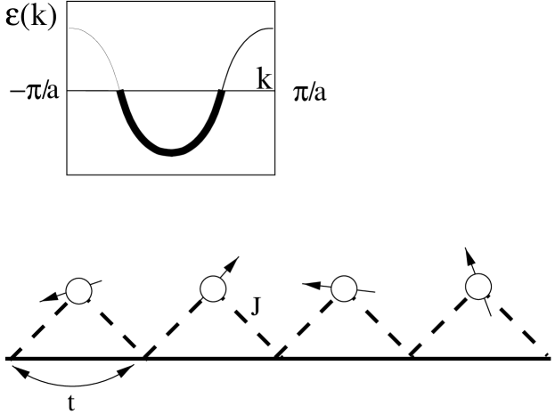
Figure 1: Illustrating the one-dimensional chain which realizes a Kondo lattice without back-scattering.

We begin by linearizing the spectrum around the Fermi energy, representing the electron on the lattice by a continuum of right and left moving electrons

$$\frac{1}{\sqrt{a}}\psi_{j\sigma}=\biggl{(}R_{\sigma}(x_{j})e^{ik_{F}x_{j}}+L_{\sigma}(x_{j})e^{-ik_{F}x_{j}}\biggr{)},$$ (2)

to obtain

$$H = H_{0}+V,$$ (3)

$$H_{0} = -\mbox{i}v_{F}\int\mbox{d}x[R^{+}_{\sigma}\partial_{x}R_{\sigma}-L^{+}_{\sigma}\partial_{x}L_{\sigma}]+(\mbox{interaction}),$$ (4)

$$V = v_{F}\sum_{j}{\bf S}_{j}\cdot\left[g_{f}({\bf J}_{R}+{\bf J}_{L})+g_{b}\left(\mbox{e}^{-2\mbox{i}k_{F}x_{j}}{\bf n}_{R}+\mbox{e}^{2\mbox{i}k_{F}x_{j}}{\bf n}_{L}\right)\right],$$ (5)

where

$$g_{f} = (J/t),$$ (6)

$$g_{b} = (J/t)\cos(k_{F}a),$$ (7)

are the dimensionless coupling constants for forward and back-scattering, $a$ is the lattice spacing and

$${\bf J}_{R}=R^{+}_{\sigma}\vec{\sigma}_{\sigma,\sigma^{\prime}}R_{\sigma^{\prime}},\>{\bf J}_{L}=L^{+}_{\sigma}\vec{\sigma}_{\sigma,\sigma^{\prime}}L_{\sigma^{\prime}},$$ (8)

define the currents of right and left moving electrons. The back-scattering term couples the spins to the components of the staggered magnetization at momentum $\pm 2k_{F}$

$${\bf n}_{R}=R^{+}_{\sigma}\vec{\sigma}_{\sigma,\sigma^{\prime}}L_{\sigma^{\prime}},\>{\bf n}_{L}=L^{+}_{\sigma}\vec{\sigma}_{\sigma,\sigma^{\prime}}R_{\sigma^{\prime}}.$$ (9)

In general this coupling can not be neglected. However, if we take the special case of half-filling, where $k_{F}a=\pi/2$, the back-scattering coefficient is identically zero and our discussion considerably simplifies. Note also that we have added an implicit electron-electron interaction term to $H_{0}$. Even though the original mode contains no explicit interactions, interactions will be generated by the high-energy physics. We shall shortly see how these implicit interaction effects can be included into the bosonized form of the Hamiltonian.

We now focus our attention on the half-filled case. Let us begin by reviewing the abelian bosonization procedure. The electron operators are written

$$\left.\begin{array}[]{c}R_{\sigma}(x)\cr L_{\sigma}(x)\end{array}\right\}={1\over\sqrt{2\pi a}}e^{-i\sqrt{4\pi}\phi^{\pm}_{\sigma}(x)}.$$ (12)

The right and left-moving electron phases $\phi^{\pm}_{\sigma}=\frac{1}{\sqrt{2}}(\phi^{\pm}_{c}+\sigma\phi^{\pm}_{s})$ can be written in terms of canonically conjugate fields

$$\phi^{\pm}_{\lambda} = \frac{1}{2}[\Theta_{\lambda}(x)\mp\Phi_{\lambda}(x)],\qquad\qquad(\lambda=c,s)$$ (13)

$$\Theta_{\lambda}(x) = \int^{x}_{-\infty}dx^{\prime}\Pi_{\lambda}(x^{\prime}),$$ (14)

where

$$[\Phi_{a}(x),\Pi_{b}(x^{\prime})]=i\delta(x-x^{\prime})\delta_{ab}.$$ (15)

The low-energy physics of the interacting chain can then be modelled by the sum of two Gaussian models for the charge and spin fields $\Phi_{c}$ and $\Phi_{s}$,

$$H^{(0)} = H^{(0)}_{c}+H^{(0)}_{s},$$ (16)

$$H^{(0)}_{c} = \frac{v_{c}}{2}\int\mbox{d}x\left[K_{c}\Pi_{c}^{2}(x)+K_{c}^{-1}[\nabla\Phi_{c}(x)]^{2}\right],$$ (17)

$$H^{(0)}_{s} = \frac{v_{s}}{2}\int\mbox{d}x\left[\Pi_{s}^{2}(x)+[\nabla\Phi_{s}(x)]^{2}\right].$$ (18)

Here, the charge and spin velocities $v_{c,s}$ are non-universal and determined by the electron interactions in the chain. The spin-stiffness $K_{s}$ is fixed by the SU(2) spin-rotation symmetry : $K_{s}=1$. $K_{c}$, the charge stiffness, sets the charge susceptibility of the electron-chain $\chi_{c}={\pi K_{c}/(2v_{c})}$. $K_{c}$ is dependent on the electron-electron interactions in the chain. If these interactions are predominantly repulsive, we expect $K_{c}<1$.

The bosonized expressions for the spin currents are then

$$J^{(+)}_{R} = J_{R}^{x}+iJ_{R}^{y}=\frac{1}{2\pi a_{0}}\exp[\mbox{i}\sqrt{2\pi}(\Theta_{s}-\Phi_{s})],$$

$$J^{(+)}_{L} = J_{L}^{x}+iJ_{L}^{y}=\frac{1}{2\pi a}\exp[\mbox{i}\sqrt{2\pi}(\Theta_{s}+\Phi_{s})],$$

$$J_{R}^{z}+J_{L}^{z} = \sqrt{\frac{2}{{\pi}}}\nabla\Phi_{s}.$$ (19)

When backscattering is absent, the charge degrees of freedom decouple. Using the expressions for currents (19) we obtain the Hamiltonian for the spin-dynamics :

$$H_{spin} = H^{(0)}_{s}+H_{int},$$ (20)

$$H_{int} = v_{s}\sum_{j}\left\{g^{z}{\sqrt{\frac{2}{\pi}}}S^{z}_{j}\nabla\Phi(j)+\frac{g^{\perp}}{2\pi a}\cos[\sqrt{2\pi}\Phi(j)]\biggl{(}S^{+}_{j}e^{-\mbox{i}\sqrt{2\pi}\Theta(j)}+{\rm H.c.}\biggr{)}\right\},$$ (21)

where we the subscripts $s$ and $f$ on the phase variables and coupling constants have been dropped for clarity. To examine the model in a solvable Toulouse limit, an easy-axis anisotropy has been included into the couplings. This model with $g^{z}>>g^{\perp}$ for a single local spin was considered by Clarke et al.[8] and is equivalent to the two-channel Kondo model.

Following Toulouse, Emery and Kivelson, we absorb the phase factor $e^{-\mbox{i}\sqrt{2\pi}\Theta(j)}$ into the spin operators by a unitary transformation, writing

$$\tau^{(\pm)}_{j}=U{{}^{{\dagger}}}S^{(\pm)}_{j}U=S^{(\pm)}_{j}e^{\mp\mbox{i}\sqrt{2\pi}\Theta(j)},$$ (22)

where

$$U=e^{\mbox{i}\sqrt{2\pi}\sum_{j}\Theta(j)S^{z}_{j}}.$$ (23)

Since $[\Theta(j),\Phi(x)]=-i\theta(x_{j}-x)$, it follows that

$$U\sqrt{2\pi}\Phi(x)U{{}^{{\dagger}}}=\sqrt{2\pi}\Phi(x)+2\pi\sum_{l}S_{l}^{z}\theta(x_{l}-x),$$ (24)

in other-words, each spin to the right of $x$ changes the spin-phase by $\pi$. This means that the electron acquires a phase of $\delta=\pi/2$ each time it scatters off a spin. This is the “resonant scattering” we expect from the physics of the Kondo effect. It also follows that

$$\frac{1}{2}\int dxU[\nabla\Phi]^{2}U{{}^{{\dagger}}}=\frac{1}{2}\int dx[\nabla\Phi]^{2}-\sqrt{2\pi}\sum_{j}\nabla\Phi(x_{j})S_{j}^{z}\ ,$$ (25)

so that

$$H^{*} = UHU{{}^{{\dagger}}},$$ (26)

$$= H^{(0)}_{s}+v_{s}\sum_{j}\biggl{\{}(g^{z}-\pi){\sqrt{\frac{2}{\pi}}}\tau^{z}_{j}\nabla\Phi(j)+(-1)^{j}\frac{g^{\perp}}{\pi a}\cos[\sqrt{2\pi}\Phi(j)]\tau^{x}_{j}\biggr{\}}.$$ (27)

To characterize the low energy physics of the ZKE model, it is convenient to examine the strongly anisotropic “Toulouse limit” where $g_{z}=\pi$, so

$$H^{*}=H^{(0)}_{s}+v_{s}\sum_{j}\frac{g^{\perp}}{\pi a}(-1)^{j}\tau^{x}_{j}\cos[\sqrt{2\pi}\Phi_{s}(j)].$$ (28)

Experience gained from the one and and two-channel Kondo models leads us to anticipate that provided the local moments are screened, then the physics of the Toulouse limit will extend extending out to the isotropic point.

3 The order parameter

In this section we discuss the correlations present in the ground-state of the ZKE model at the Toulouse point. This model is, in essence, a chain of two-channel Kondo impurities: each localized spin is coupled to the right and left-moving screening channels. In isolation, a two-channel Kondo impurity retains an unquenched degree of freedom associated with the ability of the Kondo singlet to fluctuate between the two screening channels. This residual spinless degree of freedom behaves like a localized Majorana fermion. In the ZKE model, these degrees of freedom become coupled, removing the residual entropy by generating a low-lying band of spinless excitations.

At the Toulouse point, the $\tau^{x}_{j}$ commute with the Hamiltonian, becoming constants of the motion with eigenvalues $\tau^{x}_{j}=\pm\frac{1}{2}$. In the ground-state, the spin-phase of the conduction chain prefers to acquire a constant value. The $(-1)^{j}$ coupling term in the Hamiltonian will mean that the $\tau_{j}^{x}$ develop staggered long-range order in the ground-state

$$\langle\tau^{x}_{j}\rangle=\frac{Z}{2}(-1)^{j}.$$ (29)

The effective spin Hamiltonian for the ground-state is then a sine-Gordon model

$$\tilde{H}=H^{(0)}_{s}+\frac{M_{o}}{\pi a}\int dx\cos[\sqrt{2\pi}\Phi_{s}(x)],$$ (30)

where $M_{o}=\Lambda g^{\perp}$ is the “bare” mass and $\Lambda=v_{s}/a$ is the high-energy cut-off. The “$\sqrt{2\pi}$” prefactor in the cosine guarantees that the sine-Gordon Hamiltonian (30) possesses a full SU(2)-spin symmetry (see [9]). In other-words, the formation of Kondo singlets completely quenches the anisotropy of the Kondo coupling, restoring the full symmetry of the band. From the Bethe Ansatz solution to the sine Gordon model, it is known that the spectrum of this model contains a low-lying triplet separated from the ground-state by gap $\Delta_{s}$ and a singlet with a gap $M=\sqrt{3}\Delta_{s}$ [10]. The approximate size of the spin-gap $\Delta_{s}$ can be obtained from simple scaling arguments. Since the spin phase $\Phi_{s}$ is a Gaussian variable, we know that in the uncoupled chain, $\cos(\sqrt{2\pi}\Phi)$ has a power-law correlations

$$\langle\cos(\sqrt{2\pi}\Phi(1))\cos(\sqrt{2\pi}\Phi(2))\rangle\sim\frac{1}{(\Delta x^{2}-v_{s}^{2}\Delta t^{2})^{\frac{1}{2}}},$$ (31)

corresponding to scaling dimension $d=1/2$. When we integrate out high frequency modes, rescaling $(x,t)=\lambda(x^{\prime},t^{\prime})$, where $\lambda=(\Lambda/\Lambda^{\prime})$ is the ratio of cut-off energies, we must rescale the operator

$$\cos(\sqrt{2\pi}\Phi)=\lambda^{-\frac{1}{2}}\cos(\sqrt{2\pi}\Phi^{\prime}).$$ (32)

The coupling constant then scales $g_{\perp}\rightarrow\lambda^{(2-\frac{1}{2})}g_{\perp}=g_{\perp}^{*}$. The spin gap develops at the point when strong-coupling is reached. Setting $g_{\perp}^{*}=1$, $\lambda=\frac{\Lambda}{\Delta_{s}}$, where $\Lambda=v_{s}/a$ is the upper cut-off, it follows that $\Delta_{s}\sim\Lambda(g^{\perp})^{2/3}$. This gap is much greater than the single impurity Kondo temperature $T_{K}\sim\Lambda(g^{\perp})^{2}$.

Although there is no single operator that can be directly related to the variable $\tau^{x}_{j}$, there is a collection of composite operators that are equal to $\tau^{x}_{j}$, up to a phase factor. Consider the following composite operators

$$\Psi^{+}_{j} = -{i}\biggl{(}\psi{{}^{{\dagger}}}_{j+\frac{1}{2}}\vec{\sigma}\sigma_{2}\psi{{}^{{\dagger}}}_{j-\frac{1}{2}}\biggr{)}\cdot\vec{S}_{j},$$ (33)

$$\Psi^{z}_{j} = \frac{(-1)^{j}}{2}\biggl{(}\psi{{}^{{\dagger}}}_{j+\frac{1}{2}}\vec{\sigma}\psi_{j-\frac{1}{2}}+\psi{{}^{{\dagger}}}_{j-\frac{1}{2}}\vec{\sigma}\psi{{}^{{\dagger}}}_{j+\frac{1}{2}}\biggr{)}\cdot\vec{S}_{j}.$$ (34)

The first operator describes a composite singlet formed between a local moment and a triplet pair on the neigboring sites, the second describes a singlet between the local moment and an electron delocalized on the two neighboring sites. These operators as the order parameters for odd-frequency singlet pairing and odd-frequency charge-density wave formation respectively. An expectation value $\langle\Psi^{+}_{j}\rangle$ would break gauge invariance, but it does not induce any equal-time pairing. $\Psi$ changes sign under an exchange of electron spin or position co-ordinates. The induced pair correlation function

$$F_{\alpha\beta}(x-x^{\prime},t-t^{\prime})=\langle\psi_{\alpha}(x,t)\psi_{\beta}(x^{\prime},t^{\prime})\rangle.$$ (35)

must exhibit the same symmetries, i.e.

$$F_{\alpha\beta}(x,t)=SF_{\beta\alpha}(x,t)=PF_{\alpha\beta}(-x,t),\qquad P=S=-1.$$ (36)

Since the parity for the combined operation of spin, space and time inversion is $SPT=-1$ and $SP=1$, it follows that $T=-1$, i.e the pair correlations are odd in time

$$F_{\alpha\beta}(x,t)=-F_{\alpha\beta}(x,-t).$$ (37)

$\Psi^{z}_{j}$ is obtained by taking the commutator of $\Psi_{j}^{+}$ with the staggered isospin operator ${\cal T}^{-}=\sum(-1)^{j}\psi_{j\downarrow}\psi_{j\uparrow}$, $\Psi^{z}_{j}=[{\cal T}^{-},\Psi^{+}_{j}]$. Since the action of ${\cal T}^{-}$ is to convert a singlet pairing field to a charge-density operator, it follows that an expectation value $\langle\Psi^{z}_{j}\rangle$ induces an odd-frequency charge modulation.

The long-wavelength decompositions of the composite order parameters are

$$\Psi^{+}_{j} \sim a(-1)^{j}\left[R{{}^{{\dagger}}}_{\uparrow}(x_{j})L{{}^{{\dagger}}}_{\uparrow}(x_{j})S^{-}_{j}+R{{}^{{\dagger}}}_{\downarrow}(x_{j})L{{}^{{\dagger}}}_{\downarrow}(x_{j})S^{+}_{j}\right]+\dots\ ,$$ (38)

$$\Psi^{z}_{j} \sim (a(-1)^{j}/2)\left\{\left[R{{}^{{\dagger}}}_{\uparrow}(x_{j})L_{\downarrow}(x_{j})-L{{}^{{\dagger}}}_{\uparrow}(x_{j})R_{\uparrow}(x_{j})\right]S^{-}_{j}-{\rm H.c}\right\}+\dots\ ,$$ (39)

where the terms coupling to $S_{z}$ have been omitted. We may re-write the operators appearing in these expressions using the bosonized expressions for the Fermi fields(12),

$$(-1)^{j}R^{+}_{\uparrow}(x_{j})L^{+}_{\uparrow}(x_{j})S^{-}_{j} = {i\over 2\pi a}(-1)^{j}\tau^{-}_{j}\exp[-\mbox{i}\sqrt{2\pi}\Theta_{c}],$$

$$(-1)^{j}R^{+}_{\downarrow}(x_{j})L^{+}_{\downarrow}(x_{j})S^{+}_{j} = {i\over 2\pi a}(-1)^{j}\tau^{+}_{j}\exp[-\mbox{i}\sqrt{2\pi}\Theta_{c}],$$

$$(-1)^{j}R^{+}_{\uparrow}(x_{j})L_{\downarrow}(x_{j})S^{-}_{j} = {1\over 2\pi a}(-1)^{j}\tau^{-}_{j}\exp[-\mbox{i}\sqrt{2\pi}\Phi_{c}],$$

$$(-1)^{j}R^{+}_{\downarrow}(x_{j})L_{\uparrow}(x_{j})S^{+}_{j} = {1\over 2\pi a}(-1)^{j}\tau^{-}_{j}\exp[-\mbox{i}\sqrt{2\pi}\Phi_{c}],$$

where $\tau_{j}^{\pm}=\exp[\mp\mbox{i}\sqrt{2\pi}\Theta_{s}]S^{\pm}_{j}$. Using (29), we obtain

$$\Psi^{+}_{j} \sim \frac{Z}{\pi}e^{-i\sqrt{2\pi}\Theta_{c}(j)},$$

$$\Psi^{z}_{j} \sim \frac{Z}{\pi}\sin{\sqrt{2\pi}\Phi_{c}(j)}.$$ (40)

The scaling dimensions of $e^{-i\sqrt{2\pi}\Theta_{c}}$ and $e^{-i\sqrt{2\pi}\Phi_{c}}$ are $\frac{1}{2K_{c}}$ and $\frac{K_{c}}{2}$ respectively, so that

$$\langle\Psi^{-}(1)\Psi^{+}(2)\rangle \sim \frac{1}{[\Delta x^{2}-v_{s}^{2}\Delta t^{2}]^{\frac{1}{2K_{c}}}},$$

$$\langle\Psi^{z}(1)\Psi^{z}(2)\rangle \sim \frac{1}{[\Delta x^{2}-v_{s}^{2}\Delta t^{2}]^{\frac{K_{c}}{2}}}.$$ (41)

In other words, the development of long-range order in the variable $\tau_{j}^{x}$ leads to long-range odd-frequency singlet and odd-frequency charge-density wave correlations, where $\Theta_{c}$ is the phase of the pair correlations and $\Phi_{c}$ is the phase of the charge-density wave correlations. Odd-frequency pair correlations will dominate the long-range correlations when the electron interactions are repulsive and $K_{c}<1$.

Of course, since the Toulouse limit is anisotropic, a certain amount of singlet pairing corrleations are induced, for example, the triplet order parameter

$$\phi^{t}_{j}=\biggl{[}\psi{{}^{{\dagger}}}_{j+\frac{1}{2}\uparrow}\psi{{}^{{\dagger}}}_{j-\frac{1}{2}\downarrow}-\psi{{}^{{\dagger}}}_{j-\frac{1}{2}\uparrow}\psi{{}^{{\dagger}}}_{j+\frac{1}{2}\downarrow}\biggr{]}\sim\frac{1}{2\pi}\langle\cos\sqrt{2\pi}\Phi_{s}(j)\rangle\exp[-i\sqrt{2\pi}\Theta_{c}(j)]$$ (42)

also develops long-range correlations. Since the scaling dimension of $\cos\sqrt{2\pi}\Phi_{s}$ is $d=\frac{1}{2}$, we expect $|\langle\cos\sqrt{2\pi}\Phi_{s}(j)\rangle|\sim(\Delta_{s}/t)^{\frac{1}{2}}\sim(J/t)^{\frac{1}{3}}$, so the amplitude of triplet pair correlations is reduced relative to the odd-frequency singlet correlations by a factor $(J/t)^{\frac{2}{3}}<<1$. These secondary triplet correlations are induced by the anisotropy, and will vanish in the isotropic limit.

We thus see that in the absence of back-scattering, the main characteristic of the ZKE model is the development of a spin gap and, in the case of repulsive electron-electron interactions, the establishment of long-range odd-frequency singlet pair correlations in its ground-state.

4 Excitations

Let us discuss the excitation spectrum of the Hamiltonian (30) in more detail. We assume that the spin field is locked, so that $\cos(\sqrt{2\pi}\Phi_{s})$ can be replaced by its average. This yields the following effective “magnetic” field acting on $\tau^{x}$:

$$h=\Lambda(g^{\perp})\langle\cos(\sqrt{2\pi}\Phi_{s})\rangle\sim\Lambda(g^{\perp}/a_{0})^{4/3}\sim(\Delta_{s})^{2}/\Lambda.$$ (43)

Thus the energy necessary to flip a single pseudospin is much smaller than the gap of the propagating spin excitations. Exactly at the Toulouse limit pseudospin flips do not propagate, but this changes when one considers finite $\delta g^{z}=\pi-g^{z}$. We can integrate approximately over $\Phi$ putting

$$\langle\langle\nabla\Phi_{s}(q,\omega)\nabla_{x}\Phi_{s}(-q,-\omega)\rangle\sim\chi_{s}\frac{(q)^{2}}{q^{2}+\xi^{-2}},$$ (44)

where $\chi_{s}\sim 1/\Lambda$ and $\xi=a\Lambda/\Delta_{s}$ is the correlation length. This leads to the following quantum Ising model Hamiltonian for the coupled pseudospins:

$$H=\sum_{j}[\tilde{J}(q)\tau^{z}(q)\tau^{z}(-q)]+h\sum_{j}(-1)^{j}\tau_{j}^{x},$$ (45)

where $\tilde{J}(q)=\chi(q)[\Lambda\delta g]^{2}$. We can get a rough idea of the dispersion of the pseudo-spin excitations using a Holstein-Primakov transformation $\tau^{+}_{q}=b{{}^{{\dagger}}}_{q}$, which gives a spectrum

$$\omega_{q}=\biggl{[}h(\tilde{J}(q)+h)\biggr{]}^{\frac{1}{2}}.$$ (46)

We see that in a narrow range of wavevectors $|q|<\xi^{-1}<<a^{-1}$ where $a$ is the lattice constant, $\omega_{q}\sim h$. Outside this region, $\omega_{q}\sim\Delta_{s}\bigl{[}(\delta g^{z})^{2}+(\Delta_{s}/\Lambda)^{2}]^{\frac{1}{2}}$. There are thus two gaps in the excitation spectrum:

• Spin-gap $\Delta_{s}=\Lambda(g^{\perp})^{\frac{2}{3}}$.

• Pseudo-spin gap $h=(\Delta_{s})^{2}/\Lambda$.

The lower band of spinless, dispersing excitations is most naturally interpreted as the residue of the Majorana excitations present in individual two-channel Kondo impurities.

Let us now develop a heuristic picture of the temperature dependence of the ZKE chain. At the highest possible temperatures, the individual Kondo spins are unbound, with a spin susceptibilty $\chi_{0}\sim 1/T$. A “Zhang-Rice” singlet[11] will begin to form around each spin along the chain at a characteristic scale $T^{*}$. We may estimate this scale from a high temperature expansion. At high temperatures $T>>h$,

$$\Pi\equiv\langle\langle\cos(\sqrt{2\pi}\Phi)\cos(\sqrt{2\pi}\Phi)\rangle\rangle_{\omega,q\rightarrow 0}\sim 1/T,$$ (47)

so the RPA expression for the pseudo-spin susceptibility

$$\langle\tau^{x}(-\omega,-q)\tau^{x}(\omega,q)\rangle_{\omega,q=0}=[(\chi_{0})^{-1}-(g^{\perp})^{2}\Pi]^{-1}\sim(T-\mbox{const}(g^{\perp})^{2}/T)^{-1}$$ (48)

acquires a singularity at $T^{*}\sim\Lambda g^{\perp}$. This singularity will be smeared out by fluctuations, but marks the development of Zhang-Rice singlets between the local moments and the conduction chain. For small $g^{\perp}$, $T^{*}$ is much smaller than the zero-temperature spin-gap, but much larger than the pseud-spin gap $h$, $h<<T^{*}<<\Delta_{s}$. There is thus a wide temperature region, $h(0)<<T<<T^{*}$, where the pseudo-spin band is nondegenerate, but the local spins are strongly correlated with the conduction electrons to form Zhang-Rice singlets.

5 Re-introduction of back-scattering.

We now return to discuss the back-scattering terms. We should like to be sure that our results are indeed robust against the inclusion of small amounts of back-scattering. At half-filling, we can not really turn on the interactions between the electrons in the chain, for in this case the model will become develop a charge gap. But we need to turn on the electron-electron interactions, because only then will the odd-frequency pair correlations become enhanced over the odd-frequency charge correlations. The key to this dilemma, is to dope the model away from half-filling. This introduces small amounts of back-scattering. Writing

$$n^{3}_{R,L} = -\frac{1}{2\pi a}\sin(\sqrt{2\pi}\Phi_{s})e^{\mp i\sqrt{2\pi}\Phi_{c}},$$ (49)

$$n_{R}^{\pm} = -\frac{1}{2\pi a}e^{-i\sqrt{2\pi}(\Phi_{c}\mp\Theta_{s})},$$ (50)

$$n_{L}^{\pm} = -\frac{1}{2\pi a}e^{-i\sqrt{2\pi}(-\Phi_{c}\mp\Theta_{s})},$$ (51)

the back-scattering part of the Hamiltonian may be written form

$$H_{int}=\sum_{j}\left\{\cos(\sqrt{2\pi}\Phi_{c}+2k_{F}R_{j})\left[g_{b}^{z}\tau^{x}_{j}+g_{b}^{\perp}(-1)^{j}\tau^{z}_{j}\sin[\sqrt{2\pi}\Phi_{s}(j)]\right]\right\}.$$ (52)

Although this term is oscillatory in nature, we need to examine its scaling properties to ensure that incommensurate phases do not form before odd-frequency pairing has time to develop. The scaling dimension of the back-scattering term is $K_{c}/2$ (the first term has a larger scaling dimension $(K_{c}+1)/2$, and can be neglected), so the coupling constant rescales to a renormalized value

$$g^{*}_{b}[\omega]\sim g_{b}\biggl{(}\frac{\omega}{\Lambda}\biggr{)}^{\frac{K_{c}}{2}-2}.$$ (53)

The forward scattering scales to strong coupling at at energies $\omega$ comparable with the spin gap $\Delta_{s}$. In order that odd-frequency correlations develop, we require that the renormalized backscattering coupling constant is small at this scale, i.e.

$$g^{*}_{b}[\Delta_{s}]\sim g_{b}\biggl{(}\frac{\Delta_{s}}{\Lambda}\biggr{)}^{\frac{K_{c}}{2}-2}\sim g_{b}\biggl{(}g_{f}^{\perp}\biggr{)}^{(K_{c}-4)/3}<<1,$$ (54)

where we have used $\Delta_{s}=\Lambda g_{f}^{2/3}$. But $g_{b}/g_{f}=\cos(k_{F}a)$, so that

$$\cos k_{F}a<<\biggl{(}\frac{J}{t}\biggr{)}^{(1-K_{c})/3},$$ (55)

defines the region around half-filling where we expect odd-frequency pair correlations to survive in the original model. For repulsive interactions $1/2<K_{c}<1$, so that even in the limit of infinitely strong repulsion, $K_{c}=1/2$, this condition allows for a broad range of doping. For these reasons, we expect odd-frequency pairing correlations to persist in a finite region around half-filling.

6 Discussion: into Three dimensions.

We should like to end this paper by discussing how the results of the ZKE model might extend to higher dimensional models. To assemble the chains into a three dimensional structure one may introduce a direct electron hopping $t_{\perp}$ between the chains, as shown in Fig. 2(a) We consider the case where this hopping is small: $|t_{\perp}|<<\Delta_{s}$,

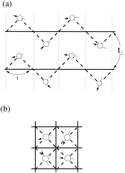
Figure 2: (a) Coupled ZKE chains. (b)“Confederate Flag” model, a symmetric generalization of the ZKE model to two dimensions. Unlike the “Zhang-Rice” singlet, where each spin couples to a single Wannier state built up out of four orbitals, here the back-scattering is absent, so that each spin has four separate antiferromagnetic links to neighboring electrons.

so that single particle hopping is virtual, but pair hopping is direct. There will be Josephson tunneling of both ordinary and composite (34) pairs, but with very different matrix elements. For ordinary pairs the hopping matrix element is $\sim t_{\perp}^{2}$, but for a composite pair in the absence of direct spin exchange between the chains it is $\sim t_{\perp}^{4}$. Taking into account Eq.(39) we get the same effective interaction in both cases:

$$V_{int}=\sum_{i\neq j}T_{ij}\tau^{x}_{i}\tau^{x}_{j}\cos[\sqrt{2\pi}(\Theta_{i}-\Theta_{j})].$$ (56)

This form of interaction was postulated by Abrahams et al. in their last paper about odd-frequency pairing [5].

If the composite order parameter has the long-range correlations in the individual chains, then the bare susceptibility for composite pairing in the system of uncoupled chains has the following frequency dependence

$$\chi^{(o)}(\omega)\sim\int dxdte^{i\omega t}(x^{2}-v_{c}^{2}t^{2})^{-\frac{1}{2K_{c}}}\sim\omega^{-2+(1/K_{c})}.$$ (57)

At a temperature $T$, the composite pair susceptibility

$$\chi^{(o)}(T)\sim T^{-2+({1}/{K_{c}})}$$ (58)

is a divergent function of temperature, providing $K_{c}>\frac{1}{2}$, a condition satisfied except in the extreme limit of repulsive interactions. For weak interchain coupling, the effective pair susceptibility $\chi(T)=[(\chi^{(o)})^{-1}-\langle T_{ij}\rangle]^{-1}$ will diverge at a temperature $T_{c}\sim\langle T_{ij}\rangle^{\eta}$ with $\eta=K_{c}/(2K_{c}-1)$, giving rise to a a macroscopically phase coherent odd-frequency superconductor.

How can we study the odd-frequency pair condensate which forms? One proposal, is to examine the limit of strong intrchain repulsion, for in this limit the superconducting order parameter has scaling dimension $(1/K_{c})\sim 2$, so it can be represented as the fermion bilinear. In this case one can describe the low-energy behaviour by 3D fermionic Hamiltonian of spinless fermions

$$H_{eff} = \sum_{j}H(j)+\sum_{i,j}T_{ij}(R^{+}_{i}L^{+}_{i}R_{j}L_{j}+H.c)],$$ (59)

$$H(j) = v_{c}\int\mbox{d}x[-\mbox{i}(R_{j}^{+}\partial_{x}R_{j}-L^{+}\partial_{x}L)-g_{0}R_{j}^{+}R_{j}L^{+}_{j}L_{j}],$$ (60)

where $g_{0}\sim\frac{1}{2}-K_{c}$. This Hamiltonian, which describes a hopping of weakly coupled preformed pairs, bears remarkable resemblence to the Hamiltonian introduced by Anderson and Chakravarthy [13] to describe the formation of the SC order parameter in cuprates. The perturbative study of this Hamiltonian may provide insights into the properties of the coupled chain system.

Another approach which seems promising, is to use a slave-fermion representation for the localized spins:

$$\vec{S}_{j}=f_{j\alpha}{{}^{{\dagger}}}\biggl{(}\frac{\vec{\sigma}_{\alpha\beta}}{2}\biggr{)}f_{j\beta},$$ (61)

together with the constraint $n_{f}(j)=1$ This representation has a local $SU(2)$ symmetry[14]. By carrying out a Hubbard Stratonovich decoupling of the Kondo interaction which respects this gauge symmetry, one may transform the Kondo interaction into the form[15]

$$J\sum_{\lambda=1,p}\vec{\sigma}_{\lambda}\cdot\vec{S}_{j}\longrightarrow\sum_{\lambda=1,p}\left\{\tilde{c}_{\lambda}{{}^{{\dagger}}}{\cal V}^{\lambda\dagger}(j)\tilde{f}_{j}+\tilde{f}_{j}{{}^{{\dagger}}}{\cal V}^{\lambda}(j)\tilde{c}_{\lambda}+\frac{1}{2J}Tr[{{\cal V}}^{\lambda\dagger}(j){\cal V}^{\lambda}(j)]\right\},$$ (62)

where

$$\tilde{f}_{j}=\left(\matrix{f_{j\uparrow}\cr f{{}^{{\dagger}}}_{j\downarrow}}\right),\qquad\tilde{c}_{\lambda}=\left(\matrix{c_{\lambda\uparrow}\cr c{{}^{{\dagger}}}_{\lambda\downarrow}}\right),$$ (63)

are the Nambu spinors for the slave fermion and the conduction electrons. ${{\cal V}}^{\lambda}(j)=i{\rm V^{\lambda}}(j)e^{i\vec{\theta}_{\lambda}(j)n_{\lambda}(j)\cdot\vec{\tau}}$ is an SU(2) matrix representing the singlet bond formed between the spin at site $j$ and its neighbor at site $\lambda$. The quantity $p$ is the number of orbitals that hybridize with the local moment. For the ZKE model, $p=2$. This Hamiltonian has the $SU(2)$ gauge symmetry

$${\cal V}^{\lambda}(j) \rightarrow g_{j}{{\cal V}}^{\lambda}(j),$$ (64)

$$\tilde{f}_{j} \rightarrow g_{j}\tilde{f}_{j},$$ (65)

where $g_{j}$ is an $SU(2)$ operator. Although ${{{\cal V}}}^{\lambda}$ is not gauge invariant, if there is more than one neighbor, then ${\cal V}^{\lambda\dagger}{\cal V}^{\lambda^{\prime}}$ is an SU(2) invariant which describes the phase coherence of the Kondo singlet between the neighboring atoms. For the ZKE model, this invariant is directly related to the two composite order parameters

$${\cal V}^{j+1\dagger}{\cal V}^{j}\propto\left[\matrix{(-1)^{j}\Psi^{z}_{j}&\Psi^{-}_{j}\cr\Psi^{+}_{j}&(-1)^{(j+1)}\Psi^{z}_{j}}\right].$$ (66)

This relation expresses the basic result that phase-coherence between a Kondo singlets that is distributed over more than one site, gives rise to odd-frequency correlations. This type of mean-field theory can be tested by checking that the mean-field theory with Gaussian fluctuations is able to reproduces the sentient feature of the ZKE bosonization. Its virtue of course lies in its ability to be generalized to a higher dimensional model. One particularly interesting model in this respect is the “confederate flag model” shown in Fig. 2(b). This model is reminiscent of the s-d models used for cuprate superconductors[11, 16], but the Kondo scattering in each plaquet has been artificially stripped of the back-scattering terms which simultaneously hop an electron and flip a spin, to create an interaction

$$H_{int}=J\vec{S}_{j}\cdot[\vec{\sigma}_{1}+\vec{\sigma}_{2}+\vec{\sigma}_{3}+\vec{\sigma}_{4}]$$ (67)

at each plaquet. It will be very interesting to see whether the removal of back-scattering does indeed give rise to coherent odd-frequency singlet pairing.

In this paper we have discussed recent non-perturbative results due to Zachar, Kivelson and Emery[6, 7] which suggest that odd-frequency pair correlations develop in a one-dimensional Kondo lattice where back-scattering is suppressed. We have introduced a simple lattice model where back-scattering is naturally suppressed, and argued that that it is odd-frequency singlet pairing that develops in this model. These correlations are robust against doping around half-filling. We have argued that when ZKE chains are coupled, this will lead to true long-range odd-frequency singlet pairing. Finally, we have proposed that the SU(2) approach to the Kondo lattice model offers a natural way to study this phenomenon in higher dimensional models.

7 Acknowledgements

We are grateful to S. Kivelson, A. Schofield and D. L. Cox for valuable discussions and illuminating remarks. This research was supported in part by the National Science Foundation under Grants No. PHY94-07194 and DMR-93-12138. P. C. and A. M. T. acknowledge a support from NATO under Research Grant CRG. 940040.

References

• [1] V. L. Berezinskii, Pis’ma v Zh.Eksp.Teor.Fiz.20, 628 (1974) [JETP Lett. 20, 287 (1974)].
• [2] A. Balatsky and E. Abrahams, Phys. Rev. B45, 13 125 (1992); E. Abrahams, A. Balatsky, J. R. Schrieffer and P. B. Allen, Phys. Rev. B47, 513 (1993).
• [3] V. J. Emery and S. A. Kivelson, Phys. Rev. B46, 10 812 (1992).
• [4] P. Coleman, E. Miranda and A. M. Tsvelik, Phys. Rev. Lett. 70, 2960 (1993), Phys. Rev. B49, 8955 (1994); Phys. Rev. Lett. 74, 1653 (1995).
• [5] E. Abrahams, A. Balatsky, D. J. Scalapino and J. R. Schrieffer, Phys. Rev. B52, 1271 (1995).
• [6] O. Zachar, S. A. Kivelson and V. J. Emery, Phys. Rev. Lett. 77, 1342 (1996).
• [7] For a more recent discussion of the ZKE approach, see V. J. Emery, S. A. Kivelson and O. Zachar, cond-mat 9610094.
• [8] D. G. Clarke, T. Giamarchi and B. I. Shraiman, Phys. Rev. B48, 7070 (1993).
• [9] F. D. M. Haldane, Phys. Rev. B25, 4925 (1982).
• [10] I. Affleck, Nucl. Phys. B265, 448 (1986).
• [11] F. C. Zhang and M. Rice, Phys Rev. B37, 3664, (1988).
• [12] A. M. Tsvelik, Sov. Nucl. Phys. ( Yad.Fis. ) 47, 172 (1988).
• [13] P. W. Anderson and S. Chakravarthy, Phys. Rev. Lett. 72, 3859 (1994).
• [14] I. Affleck, Z. Zou, T. Hsu and P. W. Anderson, Phys. Rev. B38, 745, (1988).
• [15] N. Andrei and P. Coleman, Phys. Rev. Lett. 62, 595 (1989); J. Phys Cond. Matt 1 , 4057 (1989).
• [16] S. Maekawa, T. Matsura, Y. Isawa and H. Ebisawa, Physica C 152, 133, (1988).