Absence of Translational Ordering In Driven Vortex Lattices

Abstract

By using finite temperature molecular dynamics simulations, we consider the question of the existence of dynamical ordering as a two dimensional vortex lattice is driven through a random background potential. The shape of the current-voltage($I$-$V$) characteristics are qualitatively the same as those seen in experiments on the conventional superconductors $2H$–${\rm NbSe_{2}}$ and ${\rm Mo_{77}Ge_{23}}$. However, in contrast to previous simulations, we find that the lattice has no topological or translational order for any value of the driving but that it does exhibit a high driving phase where long range orientational order exists.

I Introduction

Generic lattices that are driven through a disordered environment provide a classic example of an elastic medium that is driven through a random quenched background potential, and a particular example of these is the driven vortex lattice in dirty type II superconductors. Other examples are charge density waves in disordered conductors, fluids in porous media and motion of magnetic bubbles through a disordered medium. In the former case, the vortex lattice, which is set up when the superconducting material is placed in a magnetic field of magnitude between its upper and lower critical fields, is pinned by randomly positioned defects in the crystalline structure of the material. When an external current is driven through the material, the motion of the vortices is also impeded by the disorder in the material. This results in the existence of a depinning transition at zero temperature, below which the average velocity of the vortices (which is proportional to the voltage across the sample) is zero, while above it is finite. The depinning transition was initially suggested to be a dynamical critical phenomenon, with diverging length scales at the depinning transition, and this was treated for the case of charge density waves using mean-field elasticity theory [1]. The fact that elasticity theory was used meant that topological defects within the charge density wave (or vortex lattice) where neglected.

Several years ago, the simulations of Jensen and co-workers [2, 3] showed that as the vortex lattice was driven through a random quenched background potential, it did not depin as a single coherently moving elastic medium but, rather, the lattice began to break and flow plastically. That is to say that there were regions of the lattice that were pinned by the random potential and then channels of moving vortices would flow around them. Their simulations showed that the strength of the random potential that was required to make the lattice flow plastically vanished in the thermodynamic limit and, thus, elasticity theory would always break down. Even after taking this into consideration, elasticity theory has still been frequently used to study the depinning transition in many systems, particularly the depinning of a $d-1$ dimensional interface in a $d$-dimensional disordered environment [4].

Recently, the focus has turned away from the study of the transition itself and turned towards the physics of the moving phase. In particular, since the vortex lattice flows plastically near to the critical driving and thus will contain much topological disorder, does the system exhibit a dynamical phase transition from a low driving phase, which has a high degree of topological disorder, to a high driving phase which is topologically ordered? This question was first addressed by Shi and Berlinsky [5] and Koshelev and Vinokur [6]. Both sets of authors performed computer simulations on simple models of a two dimensional vortex lattice in a random pinning potential and both have answered the above question in the affirmative.

Subsequently, Giamarchi and Le Doussal [7] have performed analytic studies of such a system and they predicted that the high driving phase of the system is actually a moving topologically ordered glass. Subsequent to this have been further simulations by various authors, on flux line systems [8, 9, 10] and on charge density wave systems [11], most of which claim that there is a transition to a topologically ordered high driving phase.

The experimental situation is much less clear since it is difficult to examine the fine structure of the moving lattice directly and, thus, indirect methods can only be used. Experiments on bulk $2H$–${\rm NbSe_{2}}$ [12] and ${\rm Mo_{77}Ge_{23}}$ films [13] involve measuring the $I$-$V$ characteristics and then deducing the differential resistance from the data. These $I$-$V$ curves, which are carried out in the so-called peak regime [14], bare strong resemblance to early simulations of Jensen and their shape has been attributed, by the authors, to plastic flow. In the experiments of Bhattacharya and Higgins [12], they claim that the dynamical ordering in their experiments occurs when the differential resistance reaches its high driving asymptotic value, while the authors of reference [13] claim that this occurs at the peak in the differential resistivity. Since the methods used to make these claims are indirect, i.e. they are taken from the $I$-$V$ characteristics alone, simulations are a very useful tool in studying the physics of the driven system in far more detail. The simulations that we present herein show that the more correct interpretation is that of reference [12]. However, even though we show that there is a crossover between regimes at the onset of the asymptotic flux flow resistance, the high driving phase is not topologically ordered and topological defects are always frozen into the lattice structure.

The rest of the paper is outlined as follows: the model and method are presented, followed by the results, discussion and finally our conclusions. As per usual.

II Model and Method

The model we consider is that of a two dimensional array of pancake vortices. The vortices are contained within a rectangular box with periodic boundary conditions. The dimensions of the box are chosen such that its size is commensurate with the formation of a perfect triangular vortex lattice. That is to say that, for a perfect vortex lattice of lattice spacing $a_{0}$ containing $N_{v}=N_{x}N_{y}$ vortices, the dimensions of the box are $L_{x}=N_{x}a_{0}$ and $L_{y}=N_{y}a_{0}\sqrt{3}/2$, thus giving an areal density of vortices of $n_{v}=N_{v}/(L_{x}L_{y})=2/(\sqrt{3}a_{0}^{2})$. In our simulations, we set our unit of length by $a_{0}=1$ and the system contains $N_{v}=34\times 30=1020$ vortices. The vortices then interact through a pairwise Gaussian repulsive potential, such that the potential energy of the interaction between the $ith$ and the $jth$ vortex is

$$U_{vv}({\bf r_{i}}-{\bf r_{j}})=A_{v}{\rm exp}\left(-\left(\frac{|{\bf r_{i}}-{\bf r_{j}}|}{R_{v}}\right)^{2}\right)$$ (1)

where $A_{v}$ is the strength of the interaction and $R_{v}$ is its range. We set the energy scale of the simulations here by putting $A_{v}=1$. In all the simulations presented herein, the vortex-vortex interaction range is set at $R_{v}=0.6$, which corresponds to a shear modulus of $c_{66}=0.2695$ and a compression modulus of $c_{11}=1.9943$ [3].

The pinning potential in the simulations is generated by a set of $N_{p}$ randomly positioned pinning centres with positions ${\bf R_{j}^{pin}}$. The vortex-pin interaction is then given by an attractive Gaussian, such that the potential energy of the interaction between the $ith$ vortex and the $jth$ pin is

$$U_{vp}({\bf r_{i}}-{\bf R_{j}^{pin}})=-A_{p}{\rm exp}\left(-\left(\frac{|{\bf r_{i}}-{\bf R_{j}^{pin}}|}{R_{p}}\right)^{2}\right)$$ (2)

where $A_{p}$ is the strength of the interaction and $R_{p}$ is its range. The pinning parameters used in these simulations are $R_{p}=0.25$ and $A_{p}=0.5$. The density of pinning centres is $n_{p}=N_{p}/N_{v}=1$. This set of parameters ensures that the plastic flow of vortices occurs in the driven system. Let us outline the simulation method below.

From the above model parameters, we can write down a Hamiltonian for the system

$${\cal H}=\frac{1}{2}\sum_{i\neq j}U_{vv}({\bf r_{i}}-{\bf r_{j}})+\sum_{i=1}^{N_{v}}\sum_{j=1}^{N_{p}}U_{vp}({\bf r_{i}}-{\bf R_{j}^{pin}})$$ (3)

Before we simulate the $I$–$V$ characteristics of the system, we relax the vortex configuration into the pinning potential at zero driving force. Therefore, the initial conditions for the simulations of the $I$–$V$ characteristics are a relaxed lattice that already has many topological defects, rather than a perfectly ordered lattice as chosen by several other authors [5, 6]. We do this relaxation by an annealing technique using Newtonian mechanics and a rescaling of the velocities after each time step [2]. An initial temperature of $T_{i}=1$ is chosen and then the system is annealed by slowly reducing the temperature to a final value of $T_{f}=10^{-8}$. At the end of this part of the simulation, we store the vortex configuration and use it as the initial configuration for calculating the dynamical properties of the driven vortex lattice.

From the Hamiltonian above, we can then write down the equation of motion governing the over-damped dynamics of the driven system

$$\eta\frac{d{\bf r_{i}}}{dt}=-\frac{\partial{\cal H}}{\partial{\bf r_{i}}}+{\bf F_{dr}}+\chi_{i}(t)$$ (4)

the first term on the right hand side of the above equation represents the total force on vortex number $i$ due to its interaction with all the other vortices and the pins, the second term is the homogeneous driving force applied to each vortex ${\bf F_{dr}}=F_{dr}{\bf\hat{x}}$, which mimics the applied current. These first two terms make up the deterministic part of the forces, while the third term on the right hand side is a stochastic term, which has the statistical properties

$$\begin{array}[]{lll}\langle\chi_{i}(t)\rangle=0&{\rm and}&\langle\chi_{i}(t)\chi_{j}(t^{\prime})\rangle=A\delta_{ij}\delta(t-t^{\prime})\end{array}$$ (5)

Here, the angular brackets denote averages over the full distribution of random variables and the amplitude of the two-point correlator can be related to an effective temperature through $A=2k_{B}T\eta$ [15]. In these simulations we set the Boltzmann constant and the friction coefficient to $k_{B}=\eta=1$ and we use the discrete form for the stochastic forces as outlined in ref. [15].

Firstly, we perform simulations on the vortex system in the absence of pinning and at zero driving force $(A_{p},F_{dr}=0)$. We study the structure of the lattice as a function of the temperature to determine the melting scenario for the system. We measure the density of miscoordinated vortices, $n_{mis}$, derived from constructing the Voronoi Diagram for the vortex array [16], the translational order parameter,

$$\Psi_{T}=\left|\left\langle\frac{1}{N_{v}}\sum_{j=1}^{N_{v}}e^{i{\bf G}\cdot{\bf r_{j}}}\right\rangle\right|^{2}$$ (6)

and the hexatic order parameter,

$$\Psi_{H}=\left|\left\langle\frac{1}{N_{v}}\sum_{j=1}^{N_{v}}\frac{1}{z_{j}}\sum_{k=1}^{z_{j}}e^{i6\theta_{jk}}\right\rangle\right|^{2}$$ (7)

Here, both sets of angular brackets denote time averages, ${\bf G}$ is a reciprocal lattice vector, $z_{j}$ is the coordination number of vortex $j$ and $\theta_{jk}$ is the bond angle between vortex $j$ and its $kth$ neighbour relative to the fixed $x$-direction. When we calculate these quantities for the driven system, we always evaluate the quantities in the co-moving frame.

For a two dimensional lattice in the thermodynamic limit, translational order only exists at $T=0$. For any finite temperature, the long wavelength modes destroy the translational order and $\Psi_{T}=0$. However, even though long range order is absent, the translational correlation function has a power law form rather than the exponential form of an isotropic liquid. Thus, the system is said to have quasi-long range order. In continuum elasticity theory, one can write the mean squared displacements of the vortices as

$$\langle u^{2}\rangle_{th}=\frac{k_{B}T}{2\pi^{2}}\int_{0}^{k_{BZ}}\frac{d{\bf k}}{c_{66}k_{\perp}^{2}}$$ (8)

where the limit $c_{11}\gg c_{66}$ has been assumed. Thus, one can see that the divergence at ${\bf k}=0$ causes unbounded displacements which gives the loss of translational order. One can prevent this divergence by introducing a lower cut-off in the integration brought about by considering a finite sized system of linear extent $L$. The Brillouin Zone then spans the $k$-vectors $\pi/L<k<\pi/a_{0}$ and one can perform the integration to give

$$\langle u^{2}\rangle_{th}\approx\frac{k_{B}T}{c_{66}\pi}\ln\frac{L}{a_{0}}$$ (9)

i.e. bounded displacements. One can then make an estimate of a melting temperature by applying the Lindemann criterion, i.e. when the displacements are $u\sim c_{L}a_{0}$ (where $c_{L}$ is the Lindemann number), the lattice has melted. This gives a melting temperature, $T_{m}$, of

$$k_{B}T_{m}\approx\frac{c_{66}\pi(c_{L}a_{0})^{2}}{\ln\frac{L}{a_{0}}}$$ (10)

which vanishes as $L\rightarrow\infty$. One can invert the above equation to give $L_{or}(T)$. Here, $L_{or}$ is the linear size of a region (in an infinite system) over which translational order is maintained, and one can even think of the volume $L_{or}^{2}$ as being analogous to the correlated volume in collective pinning theory [17], with the size of the volume diverging as $T\rightarrow 0$. However, the above equation for the “melting” temperature (written in “ ” because it is really just a cross-over where $L_{or}$ becomes of the order of the system size) has only a very weak inverse logarithmic dependence on $L$ and thus we can expect that for macroscopic, but finite systems, a low temperature “phase” exists where translational long range order exists (again written in “ ” since it is not a true thermodynamic phase transition).

On increasing the temperature, this two dimensional solid then undergoes a melting into a liquid phase. In the Kosterlitz-Thouless type scenario for two dimensional melting, the two dimensional solid with quasi-long range order melts at a temperature $T_{m}^{KT}=0.62c_{66}a_{0}^{2}/(4\pi)$ [18], into a hexatic liquid (for the system that we consider, this is $T_{m}^{KT}\approx 0.0133$). This melting is brought about by the unbinding of dislocation pairs and the hexatic liquid is characterised by short range translational order (with $\Psi_{T}=0$ as before) and quasi-long range orientational order, i.e. $\Psi_{H}=0$ with power law hexatic correlations. At a higher temperature still, the unbound dislocations undergo a further unbinding by splitting into unbound disclination pairs. Here, both the translational and orientational order are short ranged and an isotropic liquid is formed.

We then simulate the temperature dependence of $n_{mis},\Psi_{T}$ and $\Psi_{H}$ in order to compare with the above scenario. Figure 1 shows the three quantities along with the structure factor $S({\bf k})$ for two different temperatures. One can clearly see that there is a finite temperature, $T_{m}$, at which both the translational and hexatic order parameters vanish. This also coincides with the rapid increase in the density of miscoordinated vortices in the system. The structure factors $S({\bf k})$ are shown for temperatures just above and below $T_{m}$. The system clearly undergoes a transition from a solid, signified by the set of sharp delta-function peaks, to an isotropic liquid, signified by the single $k=0$ peak and concentric rings. The peaks in the solid with quasi-long range order diverge algebraically while in the hexatic liquid, $S({\bf k})$ should display a set of concentric rings with six-fold symmetry [19, 20]. In these simulations, it seems that there is a true solid phase for low temperatures, i.e. translational and orientational order exist throughout the considered system ($L_{or}>L$), which then melts into an isotropic liquid at a finite temperature $T_{m}$. Thus, no solid with quasi-long range order or hexatic liquid are observed.

From these simulations, the melting temperature is then $T_{m}\approx 0.011$, where we have used the structure factors and order parameters as signitures of the high and low temperature phases.

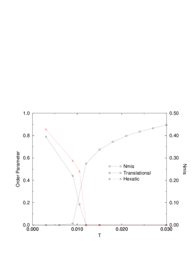
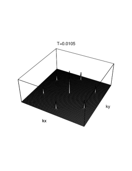
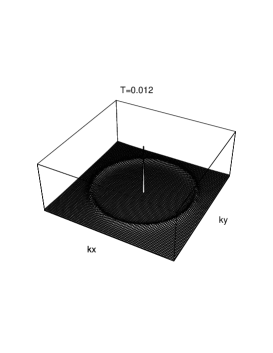
FIG. 1.: The pure, undriven system – the density of miscoordinated vortices and the translational and hexatic order parameters. Also shown are the structure factors, $S({\bf k})$, slight below and slightly above the melting transition.

From these simulations, we can choose an upper bound for the temperature at which the driven simulations are to be run, namely for temperatures below $T_{m}$. This is the obvious upper bound since, when investigating the dynamical ordering of the vortex lattice as it is driven through the pinning potential, there can clearly never be any ordering for temperatures above $T_{m}$.

We now return to the system that contains pinning in order to address the central question of this article. When driving the lattice through the random potential, we solve the set of equations 4 numerically for a particular value of the driving force. The numerical time step for the simulations is chosen as that which gives good energy conservation in the case of Newtonian dynamics (without velocity rescaling). Obviously energy will not be totally conserved in this case due to the numerical approximation. Instead, it has fluctuations around a constant average value. We chose a time step of $\delta t=0.01$, which gives a energy fluctuations of about $0.01\%$ of the average. The threshold driving force at zero temperature for the parameters stated is $F_{c}\approx 0.545$. We begin the simulations at low driving $F_{dr}=0.75$ and from the disordered configuration obtained after the initial relaxation procedure. The equations of motion are numerically iterated until the system has had time to respond to the change in driving and a steady state has been reached. For this condition to be fulfilled, we find that it is more than sufficient to solve the equations of motion until the centre of mass position of the initial vortex configuration has moved 20 lattice spacings. After this initial period, time averages are performed on the system. Time averages are performed over a minimum of 10000 time steps and until the averages have become stable to within a factor of $\pm 10^{-5}$. This always corresponds to centre of mass motion of at least 2 lattice spacings, and is usually much more.

III Results and Discussion

Here we present the results of our simulations for the set of system parameters listed above. The simulations where performed at temperatures of $T=0.0001$ and $T=0.001$, both below the melting temperature of $T_{m}\approx 0.011$.

The four graphs in Figure 2 show the differential resistance $R_{d}=d\langle v\rangle/dF_{dr}$, the fraction of vortices with average velocity $\langle v\rangle=0$, $N_{stop}/N_{v}$, the fraction of miscoordinations in the lattice, $N_{mis}/N_{v}$, and the average total pinning force, $F_{p}$, all as a function of driving force, $F_{dr}$.

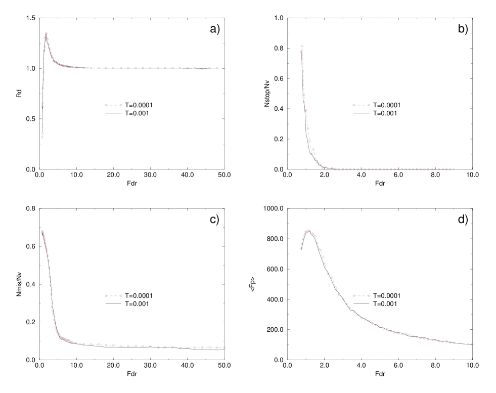
FIG. 2.: a) The differential resistance, b) The fraction of trapped vortices, c) The fraction of miscoordinated vortices, d) The average total pinning force. Results for two different temperatures, $T=0.0001$ and $T=0.001$, are shown.

The differential resistance curve is strongly resemblant of that measured in experimental systems such as $2H$–${\rm NbSe_{2}}$ [12] and those in ${\rm Mo_{77}Ge_{23}}$ thin films [13], where the $I$–$V$ characteristics have been measured in the peak regime [14]. The peak in this curve, or the fact that $R_{d}^{max}>R_{d}(F_{dr}\rightarrow\infty)$ is indicative of the existence of the prominent shoulder feature in the $I$–$V$ curve. If one examines the vortex flow patterns at driving forces around the peak in $R_{d}$, one indeed observes plastic vortex flow in channels, flowing around regions of pinned vortices. This is in agreement with the comparison between experimental curves of this form and this type of vortex flow [12]. Below we present results that show that the only feature of the dynamics of the system that can be extracted from this particular feature of the $I$–$V$ curve is that plastic flow is occurring in the vortex dynamics. One cannot determine whether or not dynamical ordering takes place in the system from this feature alone.

From figure 2a, one can see that the peak in $R_{d}$ occurs at approximately $F_{dr}\sim 1.8$. From figure 2b, one can also see that the number of trapped vortices vanishes only above a driving of $F_{dr}\sim 2.8$. From this figure we can easily conclude that, for this particular system, plastic flow definitely occurs for driving forces $F_{dr}<2.8$. It should also be noted that this is a lower bound on the threshold for plastic flow since the true definition of plastic flow is if the lattice is continually being plastically deformed as it flows, i.e. the vortices are always flowing plastically if some of the vortices are constantly changing their neighbours. We can see where the true threshold for plastic flow is by considering the distributions of the time-averaged individual vortex velocities, which are presented below.

Figure 2c shows the density of defects as a function of driving force, with the main features being the strong peak at a driving force slight greater than threshold and the asymptotic finite value of the density for large driving forces. This shows clearly an absence of a dynamical transition to a topologically ordered state and this absence is a result of hysteretic effects in the system. Depending on the initial conditions used in the simulations, one can obtain the results presented above or one can obtain the results of various other numerical works, namely that two distinct phases exist – a topologically ordered high driving phase and a disordered low driving phase which may or maybe not separated by a dynamical phase transition. Now it remains for us to decide which initial conditions are more viable. In the simulations of Shi and Berlinsky [5] and Koshelev and Vinokur [6], they began their simulations from an ordered lattice at large driving force. On reducing the driving, they then see a sharp increase in the density of defects within the vortex array. Indeed, we can observe this sort of behaviour using the same method. However, the results we present above correspond to simulations with different initial conditions. We start with a lattice configuration that is initially annealed into the pinning potential and contains a high degree of topological defects (approximately $50\%$ of the vortices are miscoordinated). The simulations then start at a driving force slightly greater than the threshold driving force which is then increased until the dynamics reach their asymptotic behaviour. We suggest that our initial conditions are more realistic and correspond to something along the lines of field-cooling a sample and then measuring the $I$–$V$ curves by increasing the external current. Thus, in these simulations we see that, rather than moving into a topologically ordered state on increasing the driving, the system moves into a state where the number of defects in the lattice become constant. It is worth noting that in ref. [13], the authors point out that a levelling off of the differential resistance at high currents is concurrent with a constant density of defects. This is indeed the case as shown by our simulations, with both quantities reaching their asymptotic values at around the same value of driving. It is also worth noting that other recent simulations [10] also observe a non-vanishing density of defects on increased driving.

The final graph, figure 2d, shows the average total pinning force as a function of $F_{dr}$. Since the physical quantities presented in figures 2a-c are all a direct consequence of the existence of the pinning force, the pinning force’s apparent insensitivity to temperature explains the insensitivity to temperature of the other quantities. We think nobody should expect that, if the pinning force was temperature independent, strong temperature dependence should be observed in the other quantities. For driving forces greater than $F_{dr}\approx 2.0$, the pinning force is independent of temperature and, in this region, one can fit the behaviour to $\langle F_{p}\rangle\sim F_{dr}^{-\alpha}$, where the exponent is $\alpha\approx 9/8$. This compares well with an exponent of unity obtained from perturbation theory [10]. The fact that $\langle F_{p}\rangle$ has a power law dependence may have consequences in the thermodynamic limit, which will be discussed later.

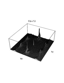
FIG. 3.: The same as in figure 1, but for the driven system. The structure factors are shown for phases with no hexatic order and for hexatic order only.

Thus, we have seen that no topological ordering takes place. This does not immediately imply there is no order whatsoever within the lattice as we know from the Kosterlitz-Thouless scenario. Figure 3 shows the density of miscoordinations, the two order parameters and the structure factors for the vortex system at a temperature of $T=0.0001$ and for various driving forces. The translational order parameter, represented by the filled circles, remains at $\Psi_{T}\approx 0$ for all driving forces, but from the hexatic order parameter, we can see that, for high driving forces, the system has some orientational order. This can also be seen from the two structure factors shown. For $F_{dr}=1.7$, $S({\bf k})$ just consists of a single peak at $k=0$ with no other structure. For the large driving forces, other peaks have appeared. The peaks are anisotropic corresponding to the anisotropic nature of the order of the lattice. We are unfortunately unable to extract the functional form of the decay of the peaks. Thus, there is a dynamical ordering that takes place, but it is not to a topologically ordered state. Finally we notice that the stucture factor for $F_{dr}=7.0$ is representative of the structure factors found at any stronger driving force. The peaks do not appear to become more narrow with increased driving.

Figure 4 shows a set of graphs showing the distribution of the time-averaged individual vortex velocities, with each graph corresponding to a different value of the driving force. For each of the $N_{v}$ vortices, we calculate the following

$$\langle v_{i}\rangle=\frac{1}{T}\int_{0}^{T}v_{i}(t)dt\approx\frac{1}{N\delta t}|{\bf r_{i}(T)}-{\bf r_{i}(0)}|$$ (11)

i.e. the angular brackets denote a time average and the subscript $i$ denotes the fact that a spatial average has not been performed. The figures in 4 then show the distributions of these quantities. Looking at the figures, one sees precisely what one would expect for plastic flow occurring in the system. Slightly above threshold ($F_{dr}=0.9$) the distribution consists of a strong peak at $\langle v\rangle=0$, with some small but finite velocities having lower weights, i.e. most of the vortices are trapped for this value of the driving, with the few moving ones contributing towards the average centre of mass velocity of the whole vortex system. The following graphs for driving $F_{dr}<2.8$ are qualitatively similar, with the peak at $\langle v\rangle=0$ decreasing and a second peak at finite velocities developing as the driving increases. This continues until $F_{dr}\approx 2.8$, where the peak at $\langle v\rangle=0$ vanishes and all the vortices become depinned. This is consistent with the result in figure 2b. The figures corresponding to $F_{dr}>2.8$ thus consist of a broad distribution with a single maximum. The position and the height of the maximum of the distribution both increase correspondingly with the driving force, and the width of the distribution, which we call $\Delta\langle v\rangle$, clearly decreases on increased driving. The fact that these distributions are of finite width ($\Delta\langle v\rangle\neq 0$) is the singular most important fact in determining whether or not the vortex array is flowing plastically and is therefore of importance when addressing the question of whereabouts dynamical ordering occurs.

FIG. 4.: The distribution of time-averaged velocities

For the vortex array to undergo a dynamical transition to a topologically ordered state at some value of the driving force, all free topological defects within the lattice must vanish and the lattice must also clearly return to the regime where only elastic deformations exist. If plastic flow exists then topological defects will be constantly appearing and disappearing. Thus, as we have seen from figure 2c that topological defects are always present, we need to tie in all the results presented above to develop an overall picture of the dynamics. From figure 2b we have stated that, for $F_{dr}<2.8$, some regions of the vortex lattice are permanently trapped while the other vortices flow aroung them. Thus for driving forces in the range $F_{c}<F_{dr}<2.8$, plastic flow occurs with some of the vortices being permanently pinned. This is in contrast to the work of ref. [10] which states that some of the vortices only remain pinned for a finite length of time. If one was to plot the instantaneous distribution of vortex velocities, one would see the double peaked structure, similar to ours, but on plotting the distribution of time-averaged velocities, the double peaked form may disappear or simply the $\langle v_{i}\rangle=0$ peak must move to a finite velocity. The fact that the distributions presented above are time-averaged and show a double peaked structure with one peak at $\langle v_{i}\rangle=0$ can only lead to the conclusion that these simulations show that the channel structures that are formed, along which the plastic flow occurs, are ‘frozen’ in. This may, of course, not necessarily be a unique structure dependent only on the value of the driving force, but probably will be dependent on the history of the system.

Therefore, we know that, for $F_{dr}>2.8$, all of the vortices are depinned, i.e. $\langle v_{i}\rangle>0$ $\forall i$. However, this does not imply that plastic flow has ceased. Here we return to the distributions of figure 4. For all plastic flow in the vortex dynamics to be truly eradicated, the infinite time-averaged velocity distribution must be a delta function, i.e. all velocities are the same and the system must be in the elastic regime. Obviously this is not the case for the time-averages in the simulations. For finite time-averages the width of the velocity distribution can be finite and still no plastic flow occurs over the time span. Thus, if the average is performed over a time $T$ and the width of the velocity distribution is $\Delta\langle v\rangle$, then one can say that the corresponding width of the distribution of distances moved during the time span of the average has a width of $\Delta x\approx\Delta\langle v\rangle T$. We can then say that, for no plastic flow to occur in the simulation, $\Delta x<a_{0}/2$. Thus, say for a time average performed over 10000 steps (remember $\delta t=0.01$), plastic flow will always occur in this time window if the width of the velocity distribution is $\Delta\langle v\rangle>\Delta\langle v\rangle_{pl}=0.005$. For the simulations presented herein, the time-averages are always performed over a time $T\geq 10000\delta t=100$ and, thus, $\Delta\langle v\rangle_{pl}=0.005$ is an upper bound for our simulations, i.e. any distribution width taken from these simulations that is greater than this corresponds to plastic flow. Thus we are in a position to tell when then vortex system has returned to the elastic regime.

From figure 4, one can see that the width of all the velocity distributions is greater than this threshold for plastic flow. In fact, only as the driving force $F_{dr}$ approaches a numerical value of $\approx 10$ does the width $\Delta\langle v\rangle$ become less than the threshold. Thus, to bring together all the results above, we can present the following picture.

The dynamics above threshold can be split into two ‘phases’, with one of these phases being split into two ‘sub-phases’. Figure 5 shows the scenario that we present as a schematic diagram. The first phase is for driving forces in the range $F_{c}<F_{dr}<F_{2}$ ($F_{c}\approx 0.545$, $F_{2}\approx 10$), where the vortices flow plastically and the phase can be defined through a non-zero width of the time-averaged individual vortex velocity distribution (presented in figure 4), $\Delta\langle v\rangle>0$. This phase is then split into two sub-phases. These are separated by a threshold $F_{1}\approx 2.8$, which is the second depinning force. The first depinning force is simply that which separates phases of zero and non-zero centre of mass velocity, i.e. $F_{c}$. $F_{1}$ signifies the point where all of the vortices become depinned. For $F_{c}<F_{dr}<F_{1}$, some vortices are moving but some are permanently pinned ($\langle v\rangle_{i}=0$) and thus $N_{stop}>0$. For $F_{1}<F_{dr}<F_{2}$, all the vortices have finite time-averaged velocities but the width of the velocity distribution is finite, signifying plastic flow.

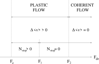
FIG. 5.: The dynamical ‘phases’ of the driven vortex system. For the simulations presented herein, $F_{c}\approx 0.545$, $F_{1}\approx 2.8$ and $F_{2}\approx 10$. See the text for a more comprehensive explanation.

The second phase is for $F_{dr}>F_{2}$ and is defined through $\Delta\langle v\rangle=0$. Here, all plastic flow has ceased and the vortex array moves as a single coherent structure. That is to say that all the vortices keep the same neighbours throughout the simulation. Here we use the phrase ‘single coherent structure’ as opposed to saying that the system has returned to the elastic regime in order to avoid any association the reader might make between an elastic regime and a topologically ordered structure.

Given that these are the different regimes of dynamics in these simulations, we now compare how the time-averaged quantities vary in each of these regimes. The quantities of interest are the density of miscoordinations, the two order parameters and the differential resistance. Firstly, looking at figure 2a, one can see that the only feature of the differential resistance that correlates with the regimes described above is that the onset of the asymptotic flux flow value of the resistance coincides with the third regime (starting at $F_{dr}\approx 10$), i.e. where the plastic flow in the system ceases. A similar thing can be said about the density of defects. The flattening off of the defect density also coincides with the onset of this regime. Thus, our main statement of the work is the following:

There is a lack of a dynamical transition to a topologically ordered state in two dimensional vortex lattices with strong pinning. However, there are two possible dynamical regimes that can be distinguished. The first is a low driving regime, where the vortices flow plastically defined through $\Delta\langle v\rangle>0$ (pinned regions may or may not exist). Here the differential resistance and the density of defects vary strongly with the driving force. The second regime is the high driving regime. Here, the vortex array moves as a single coherent structure ($\Delta\langle v\rangle=0$), i.e. all plastic flow has ceased, and the vortex dynamics have reached their asymptotic behaviour, i.e. the differential resistance and the density of defects are independent of the driving force. Since all plastic flow has ceased in this phase, the defects that remain in the lattice are frozen in. This is also reflected in the fact that the translational order parameter is zero for all driving forces. Thus, the high driving phase is not a topologically ordered phase, but one where the vortex lattice is a single coherently moving topological glass. However, even though we have shown that no topological or translational order exist at any driving force, for large enough driving forces the system exhibits long range orientational order, given by $\Psi_{H}\neq 0$.

IV Conclusions

Let us now consider the discrepancy between the simulations in this article and some recent simulations by other authors [5, 6, 8, 9, 10]. The majority of these simulations see quite a sharp dynamical transition to a topologically ordered state at some value of the driving force, which is in complete contrast with the simulations herein. We suggest that this is either an artifact of the weak pinning strengths that these simulations have used or an artifact of the initial conditions, as mentioned previously (the topological ordering observed by some authors is truly an artifact of their initial conditions since they are rather unrealistic initial conditions). Here, like most other authors, we are guilty of making a distinction between weak and strong pinning. In the thermodynamic limit this distinction becomes meaningless. In the early simulations of Jensen and co-workers [2], they showed that the pinning strength required to produce plastic flow in the system vanishes logarithmically as the thermodynamic limit is approached and, thus, the system is always in the plastic flow regime [21]. We suggest that the same effect could happen here and, thus, the dynamical ordering seen in other simulations is simply a finite size effect.

We have also stated here that, on increased driving, our simulations return to a regime where plastic flow ceases. Admittedly, this could well be a finite time effect since we have stated previously that, in the limit of infinite times, the distribution of time-averaged velocities must be a $\delta$-function for all plastic flow to cease. Thus, only when the width of the distribution does vanish will plastic flow truly cease. It is also worth noting that this may never occur. We have shown that the average pinning force never vanishes, i.e. it behaves as $\langle F_{p}\rangle\sim 1/F_{dr}$. This shows that the asymptotic flux flow resistivity is never actually reached in this model and, for infinite systems and times, any finite pinning force is capable of producing plastic flow.

Thus, we suggest the following. The simulations in this article have still not completely resolved all the questions as to dynamical ordering in vortex lattices. What is needed is a detailed finite size study of the dynamical regimes and topological phases of the lattice so that a coherent picture of the dynamical behaviour for the infinite system can be evaluated. We have shown that, for our system sizes, topological and translational order do not exist and we believe that considering larger systems will not change this [2]. However, we have observed a low driving phase without orientational order and a high driving phase with orientational order. From a purely theoretical point of view, it would be interesting to see whether or not these phases persist in the thermodynamic limit and whether or not they are separated by a true dynamical transition. We have suggested, above, that plastic flow may persist for all driving forces in the infinite lattice. From the figures presented herein, we can also see that the onset of hexatic order overlaps with the region where plastic flow occurs. Thus, we can suggest that plastic flow does not destroy the hexatic order and that this order could easily persist in infinite systems. Once the physics of the infinite system is realised, the discrepancies between our simulations and many others could probably be easily resolved.

V Acknowledgements

We wish to thank V. M. Vinokur for some very interesting and helpful discussions relating to the work and to his paper in ref. [6]. One of us (SS) would also like to acknowledge the EPSRC and DRA Malvern for financial support and the other (HJJ) was supported by the EPSRC under grant no. Gr/J 36952.

$\dagger$ Address from 15 November 1996: Department of Chemistry, The University of Cambridge, Lensfield Road, Cambridge CB2 1EW, UK

REFERENCES

- [1] D. S. Fisher, Phys. Rev. B 31, 1396 (1985)
- [2] H. J. Jensen, A. Brass and A. J. Berlinsky, Phys. Rev. Lett. 60, 1676 (1988); A. Brass, H. J. Jensen and A. J. Berlinsky, Phys. Rev. B 39, 102 (1989)
- [3] H. J. Jensen in Phase Transitions and Relaxation in Systems with Competing Energy Scales, Ed. T. Riste and D. Sherrington, (Kluwer Academic, Dordrecht 1993)
- [4] H. Leschhorn, T. Nattermann, S. Stepanow and L-H Tang, cond-mat preprint 9603114, to appear in Annalen der Physik
- [5] A-C. Shi and A. J. Berlinsky, Phys. Rev. Lett. 67, 1926 (1991)
- [6] A. E. Koshelev and V. M. Vinokur, Phys. Rev. Lett. 73, 3580 (1994)
- [7] T. Giamarchi and P. Le Doussal, Phys. Rev. Lett. 76, 3408 (1996)
- [8] K. Moon, R. T. Scalettar and G. T. Zimányi, Phys. Rev. Lett. 77, 2778 (1996)
- [9] S. Ryu, M. Hellerqvist, S. Doniach, A. Kapitulnik and D. Stroud, cond-mat preprint 9606126
- [10] M. C. Faleski, M. C. Marchetti and A. A. Middleton, cond-mat preprint 9605053
- [11] L-W. Chen, L. Balents, M. P. A. Fisher and M. C. Marchetti, cond-mat preprint 9605007
- [12] S. Bhattacharya and M. J. Higgins, Phys. Rev. Lett. 70, 2617 (1993)
- [13] M. C. Hellerqvist, D. Ephron, W. R. White, M. R. Beasley and A. Kapitulnik, Phys. Rev. Lett. 76, 4022 (1996)
- [14] A. B. Pippard, Phil. Mag. 19, 217 (1969)
- [15] A. Brass and H. J. Jensen, Phys. Rev. B 39, 9587 (1989)
- [16] F. P. Preparata and M. I. Shamos, Computational Geometry: An Introduction, (Springer-Verlag, New York 1985)
- [17] Blatter G, Feigel’man M V, Geshkenbein V B, Larkin A I and Vinokur V M, Rev. Mod. Phys. 66, 1125 (1994)
- [18] D. S. Fisher, Phys. Rev. B 22, 1190 (1980)
- [19] D. R. Nelson in Phase Transitions and Critical Phenomena, Vol. 7, Ed. C. Domb and J. L. Lebowitz, (Academic Press, 1983)
- [20] M. Franz and S. Teitel, Phys. Rev. B 51, 6551 (1995)
- [21] S. N. Coppersmith, Phys. Rev. Lett. 65, 1044 (1990)
- [22] E. H. Brandt in Phase Transitions and Relaxation in Systems with Competing Energy Scales, Ed. T. Riste and D. Sherrington, (Kluwer Academic, Dordrecht 1993)