Flux noise in high-temperature superconductors

Abstract

Spontaneously created vortex-antivortex pairs are the predominant source of flux noise in high-temperature superconductors. In principle, flux noise measurements allow to check theoretical predictions for both the distribution of vortex-pair sizes and for the vortex diffusivity. In this paper the flux-noise power spectrum is calculated for the highly anisotropic high-temperature superconductor Bi₂Sr₂CaCu₂O_8+δ, both for bulk crystals and for ultra-thin films. The spectrum is basically given by the Fourier transform of the temporal magnetic-field correlation function. We start from a Berezinskii-Kosterlitz-Thouless type theory and incorporate vortex diffusion, intra-pair vortex interaction, and annihilation of pairs by means of a Fokker-Planck equation to determine the noise spectrum below and above the superconducting transition temperature. We find white noise at low frequencies $\omega$ and a spectrum proportional to $1/\omega^{3/2}$ at high frequencies. The cross-over frequency between these regimes strongly depends on temperature. The results are compared with earlier results of computer simulations.

I INTRODUCTION

It is well known that the layered structure of cuprate high-temperature superconductors (HTSC’s) leads to enhanced two-dimensional fluctuations. These fluctuations are partly due to spontaneously created pancake vortex pairs in the superconducting CuO₂ layers. There are several attempts[2] to describe these vortices starting from the Berezinskii-Kosterlitz-Thouless (BKT) renormalization group theory.[3] These approaches differ in their predictions so that experiments are needed to decide between them.

Most experiments designed to test the predictions of BKT-type theories indirectly measure the temperature dependence of the renormalized interaction. This quantity can be obtained from the exponent $\alpha$ of the non-linear current-voltage characteristics $V\propto I^{\alpha}$.[4, 5] A second approach is to measure the linear resistivity above $T_{c}$, which is related to the superconducting correlation length. It has been shown, however, that the derivation of the resistivity within the framework of BKT theory is at best only valid in a narrow temperature range, which is probably inaccessible experimentally.[6] Thus, most of our experimental knowledge about vortex pair fluctuations is based on measurements of the temperature dependence of just one quantity. Alternative approaches would be very welcome.

Apart from the renormalized interaction and the correlation length, BKT-type theories also predict the temperature- and size-dependent fugacity of pairs, and, consequently, the distribution of pair sizes and the total pair density—at least below the transition temperature. A generalized approach[7] yields quantitative results even above $T_{c}$. It takes care of the correct counting of overlapping vortex-antivortex pairs and takes local-field effects in the screened interaction into account. In this way terms of higher order in the vortex fugacity $y$ are introduced into the Kosterlitz recursion relations,[3] facilitating a description of the vortex system even above $T_{c}$.

Only few experiments sensitive to the pair density have been performed, most of them on magnetic-flux noise. In the absence of an external magnetic field, the flux at the surface of an HTSC sample is due to the vortices in the bulk. This flux is noisy since these vortices perform a diffusive motion, carrying their magnetic field with them. Only few of these experiments have been done on HTSC’s, mostly on bulk YBa₂Cu₃O_6+δ (Y-123).[8] However, BKT-type theories and hence the approach presented here are probably not applicable to Y-123 since its anisotropy is too small. There are also noise measurements on Josephson junction arrays.[9] These arrays are discrete systems with a relatively large lattice constant, for which the continuum approach presented below is not suitable.

Rogers et al.[10] perform experiments on very thin films of Bi-2212 in the absence of an external magnetic field. (Apparently experiments on bulk single crystals of Bi-2212 have not been performed yet.) The authors find a flux-noise spectrum following a $\omega^{-3/2}$ law for frequencies $\omega\gtrsim\omega_{c}$, where the characteristic frequency $\omega_{c}$ strongly increases with temperature.

In this paper we determine the effect of vortex-pair fluctuations in both bulk HTSC’s and ultra-thin films (containing one CuO₂ layer) on flux noise. To be specific, we consider the highly anisotropic compound Bi₂Sr₂CaCu₂O_8+δ (Bi-2212) in a vanishing external magnetic field under the assumption that the superconducting layers are coupled only weakly so that the dynamics of the vortices in one layer is independent of that in the other layers. We further assume a large density of similar pinning centers. We will find that the spectral density of flux noise is governed by the temporal magnetic-field correlation function. Interestingly, the same correlation function also governs the contribution of vortex-pair fluctuations to nuclear-spin relaxation,[11, 12] albeit at much higher frequencies.

Ambegaokar et al.[13] employ a Fokker-Planck equation to obtain the linear response of a superfluid film to substrate oscillations. In this equation the authors include the interaction between vortices within the same pair. Similarly, we also start from a Fokker-Planck equation. However, we solve this equation to obtain the full space- and time-dependent vortex correlations needed for the calculation of the magnetic-field correlation function.

A similar vortex system is studied by Houlrik et al.[14] They derive a relation between the flux-noise power spectrum and the dissipation due to the vortices described by a dielectric constant $\epsilon$. This relation is valid in the limiting case of a large pick-up coil, i.e., for the flux through a large area. Houlrik et al.[14] perform computer simulations on a generalized two-dimensional, discrete XY model[15] to obtain $\epsilon$. The mentioned relation is employed to get the noise spectrum. It falls off as $1/\omega^{2}$ at very high frequencies $\omega$ and shows a $1/\omega^{3/2}$ dependence for smaller $\omega$. The $\omega^{-3/2}$ power law is in agreement with Minnhagen’s phenomenological approach.[16] In the present paper results for a continuous two-dimensional Coulomb gas model are obtained by direct calculation as opposed to simulations. Furthermore, we consider the opposite limiting case of a small pick-up coil.

The present paper is organized as follows: In Sec. II we define the flux noise power spectrum and express it in terms of a magnetic-field correlation function. In Sec. III we present a model which enables us to calculate this function and in Sec. IV we discuss our results.

II THE FLUX NOISE POWER SPECTRUM

We have the following setup in mind: The small pick-up coil of a SQUID (superconducting quantum interference device) magnetometer is placed at the surface of a large HTSC single crystal or of an extended one-unit-cell-thick film. For epitactically grown samples, the most natural way to mount the input coil is on a $\{001\}$ ($ab$) plane, sensitive to the field perpendicular to the layers. In the following we restrict ourselves to this case. The flux signal is measured in the absence of any external field or driving force. The spectrum is then obtained by Fourier transformation.

The flux-noise power spectrum $S_{\phi}$ is given by the Wiener-Khinchin theorem,[17]

$$S_{\phi}(\omega)=\frac{2}{\pi}\int_{0}^{\infty}\!\!dt\;\overline{\phi(t)\phi(0)}\,\cos\omega t.$$ (1)

Here, $\phi(t)$ is the flux through the effective area $A_{\text{eff}}$ of the input coil. If the diameter of the effective area is smaller than the typical length scale of magnetic field changes, $\lambda_{ab}$, the field is approximately uniform over the area $A_{\text{eff}}$, and we can write

$$S_{\phi}(\omega)=\frac{2}{\pi}A_{\text{eff}}^{2}\int_{0}^{\infty}\!\!dt\,\tilde{k}_{zz}(t)\cos\omega t\equiv\sqrt{\frac{2}{\pi}}\,A_{\text{eff}}^{2}\,\tilde{k}_{zz}(\omega).$$ (2)

We have thus reduced the problem to the determination of the Fourier transform of the magnetic-field correlation function

$$\tilde{k}_{zz}(t)=\overline{h_{0,z}({\bf r},t)h_{0,z}({\bf r},0)},$$ (3)

where $h_{n,z}({\bf r},t)$ is the $z$ component of the total magnetic field at the point ${\bf r}$ in layer $n$ at the time $t$.

III MODEL

A General considerations

In this section we present a model for the time-dependent local magnetic field in a layered superconductor in the absence of an external field. Results for a single layer are then obtained by means of a straightforward generalization. We assume that the Josephson coupling between the superconducting layers can be neglected as far as the dynamics of pancake vortices is concerned. Then the local field is due to spontaneously created pancake vortices in the layers. We assume that there are $N$ vortices and $N$ antivortices in each layer at any time, thus neglecting fluctuations of the vortex number. This is justified since we are only interested in the thermodynamic limit.

We decompose the vortex system into the smallest possible vortex-antivortex pairs, using the enumeration algorithm given by Halperin,[18] i.e., we count the vortex and the antivortex with the smallest separation as a pair and then repeat this step for the remaining vortices and antivortices. Let ${\bf H}_{n}({\bf r})$ be the magnetic field of a single vortex situated at the origin in layer zero measured at the point ${\bf r}$ in the $n$-th layer. Here, we only need the $z$ component of the field. It is given by[19]

$$H_{n,z}({\bf r})=\!\frac{\phi_{0}s}{4\pi\lambda_{ab}^{2}\sqrt{r^{2}+n^{2}s^{2}}}\exp\!\left(-\frac{\sqrt{r^{2}+n^{2}s^{2}}}{\lambda_{ab}}\right),$$ (4)

where $\phi_{0}$ is the superconducting flux quantum and $s$ is the interlayer spacing. This expression holds for an infinite stack of superconducting layers. The field differs from this result outside the crystal, where it is not screened. However, if the pick-up coil is placed close to the surface the difference should be negligible. The two-dimensional symmetric Fourier transform of Eq. (4) is

$$H_{n,z}({\bf k}) = \frac{\phi_{0}s}{4\pi\lambda_{ab}^{2}}\,\frac{1}{\sqrt{k^{2}+\lambda_{ab}^{-2}}}\exp\!\left(-|n|\,s\sqrt{k^{2}+\lambda_{ab}^{-2}}\right).$$ (5)

For now we only utilize the fact that the field of an antivortex is just the negative of ${\bf H}_{n}({\bf r})$. The fields of the vortices and antivortices are superposed to obtain the total magnetic field ${\bf h}_{n}({\bf r},t)$, which depends on time only through the positions of the vortices and antivortices.

We are interested in the correlation function $\tilde{k}_{zz}(t)$ as given by Eq. (3). The total magnetic field in layer zero is

$${\bf h}_{0}({\bf r},t) = \sum_{n=1}^{\infty}\sum_{\nu=1}^{N}\Big{(}{\bf H}_{n}[{\bf r}-{\bf r}_{-n,\nu+}(t)]$$ (8)

$${}-{\bf H}_{n}[{\bf r}-{\bf r}_{-n,\nu-}(t)]\Big{)},$$

where ${\bf r}_{n,\nu+}(t)$ (${\bf r}_{n,\nu-}(t)$) is the position of the vortex (antivortex) of the $\nu$-th pair in layer $n$ at the time $t$. We now assume that inter-pair correlations are negligible as compared with intra-pair correlations. We keep the correlations between the fields of the vortex and the antivortex of the same pair, however. This approximation is justified if the typical pair size is small as compared with the average distance between neighboring pairs. Under the same condition the (extended) BKT theory[7] is applicable. If we further assume diffusive dynamics we can write down the following ansatz for the correlation function:[11]

$$\tilde{k}_{zz}(t) = \frac{2N}{F}\sum_{n=1}^{\infty}\int d^{2}r_{+}^{\prime}d^{2}r_{-}^{\prime}d^{2}r_{+}d^{2}r_{-}\,$$ (12)

$$\times\big{[}H_{n,z}({\bf r}-{\bf r}_{+}^{\prime})\,H_{n,z}({\bf r}-{\bf r}_{+})$$

$$\quad{}-H_{n,z}({\bf r}-{\bf r}_{+}^{\prime})\,H_{n,z}({\bf r}-{\bf r}_{-})\big{]}$$

$$\times P({\bf r}_{+}^{\prime},{\bf r}_{-}^{\prime};{\bf r}_{+},{\bf r}_{-};t)\,f({\bf r}_{+}-{\bf r}_{-}).$$

Here, $f({\bf r})$ is the normalized distribution function of the pair separation vector ${\bf r}={\bf r}_{+}-{\bf r}_{-}$. We obtain this function numerically from the extended BKT theory of Refs. [7] and [12]. For our calculations we use an approximate form of $f({\bf r})$, which incorporates the essential physics, cf. Subsec. III C. The diffusive motion of the pairs is described by the time-evolution kernel or diffusion function $P$: $P({\bf r}_{+}^{\prime},{\bf r}_{-}^{\prime};{\bf r}_{+},{\bf r}_{-};t)\,d^{2}r_{+}^{\prime}d^{2}r_{-}^{\prime}$ is the probability of finding the vortex of a given pair in the area element $d^{2}r_{+}^{\prime}$ about ${\bf r}_{+}^{\prime}$ and the antivortex of the same pair in $d^{2}r_{-}^{\prime}$ about ${\bf r}_{-}^{\prime}$ at the time $t$ provided that the vortex was at ${\bf r}_{+}$ and the antivortex at ${\bf r}_{-}$ at the time zero. The indices $n$ and $\nu$ of the vortex positions have been omitted in Eq. (12) since we are dealing with one representative pair.

B The diffusion function

It may be instructive to turn briefly to the case of unbound pairs. In this case the vortices diffuse independently and the diffusion function separates into a product of free diffusion functions for the two partners of the pair,

$$P({\bf r}_{+}^{\prime},{\bf r}_{-}^{\prime};{\bf r}_{+},{\bf r}_{-};t) = \frac{1}{4\pi Dt}\,\exp\!\left(-\frac{|{\bf r}_{+}^{\prime}-{\bf r}_{+}|^{2}}{4Dt}\right)\;$$ (14)

$${}\times\frac{1}{4\pi Dt}\,\exp\!\left(-\frac{|{\bf r}_{-}^{\prime}-{\bf r}_{-}|^{2}}{4Dt}\right)\!,\!\!\!\!$$

where $D$ is the diffusion constant of a free vortex. By rewriting Eq. (14) in terms of center-of-mass and relative coordinates, we can see that the center of mass diffuses freely with the diffusion constant $D_{\text{CM}}=D/2$, whereas the separation vector diffuses with $D_{\text{rel}}=2D$.

Now we wish to take two important effects into account, namely the interaction between the two partners of a pair and the recombination of pairs. The latter effect is expected to destroy the correlation on the time scale of the recombination time. The center of mass of the pair should perform a free diffusion. The time-evolution kernel can then be written as

$$P\left({\bf R}^{\prime}+\frac{{\bf r}^{\prime}}{2},{\bf R}^{\prime}-\frac{{\bf r}^{\prime}}{2};{\bf R}+\frac{{\bf r}}{2},{\bf R}-\frac{{\bf r}}{2};t\right)$$ (16)

$$=\frac{1}{2\pi Dt}\,\exp\!\left(-\frac{|{\bf R}^{\prime}-{\bf R}|^{2}}{2Dt}\right)\>P_{\text{rel}}({\bf r}^{\prime},{\bf r};t).$$

The task at hand is to determine the time evolution of the separation vector, $P_{\text{rel}}({\bf r}^{\prime},{\bf r};t)$.

To obtain $P_{\text{rel}}$ we solve a Fokker-Planck equation containing the intra-pair interaction $V$.[13] The vortex-antivortex interaction is given by[3]

$$V(r)=\int_{r_{0}}^{r}\!\!dr^{\prime}\,\frac{q^{2}}{\epsilon(r^{\prime})r^{\prime}}.$$ (17)

For most pairs the dielectric constant $\epsilon(r)$ is close to unity[7] so that we may replace $q^{2}/\epsilon$ by $q^{2}$ and write $V(r)\approx q^{2}\,\ln(r/r_{0})$. The error thereby incurred turns out to be small as compared with errors due to, e.g., the uncertainty of the diffusion constant. Our approximation is best justified for small pairs, for which the interaction is screened only weakly. For temperatures significantly above $T_{c}$ many large pairs with strongly screened interaction exist and the approximation breaks down, while the extended BKT theory also becomes invalid.

If the mobility and diffusivity are isotropic and constant in space and time, the diffusion (Fokker-Planck) equation in the presence of a potential $V$ reads[17]

$$\frac{\partial P_{\text{rel}}}{\partial t}=\mu_{\text{rel}}P_{\text{rel}}\Delta V+\mu_{\text{rel}}({\mbox{\boldmath$\nabla$}}V)\cdot{\mbox{\boldmath$\nabla$}}P_{\text{rel}}+D_{\text{rel}}\Delta P_{\text{rel}},$$ (18)

where the mobility $\mu_{\text{rel}}$ is related to the diffusion constant through the Einstein relation $\mu_{\text{rel}}=D_{\text{rel}}/k_{B}T$. The initial condition is $P_{\text{rel}}({\bf r},{\bf r}_{0};0)=\delta({\bf r}-{\bf r}_{0})$. Inserting the logarithmic potential we find

$$\frac{\partial P_{\text{rel}}}{\partial t}=2\pi\mu_{\text{rel}}q^{2}\delta({\bf r})P_{\text{rel}}+\mu_{\text{rel}}q^{2}\frac{{\bf r}}{r^{2}}\cdot{\mbox{\boldmath$\nabla$}}P_{\text{rel}}+D_{\text{rel}}\Delta P_{\text{rel}}.$$ (19)

The first term on the right-hand side contains a delta function. This term yields a positive contribution to the time derivative only at ${\bf r}=0$. Therefore, it causes a $\delta$-function term to appear in $P$ at ${\bf r}=0$. Such a contribution does not affect $P$ for ${\bf r}\neq 0$. Since “pairs” with ${\bf r}=0$ are recombined and do not contribute to the magnetic field, we may omit the first term in Eq. (19). After introduction of polar coordinates, the diffusion equation can be solved by means of a separation ansatz,[12]

$$P_{\text{rel}}({\bf r}^{\prime},{\bf r};t) = \frac{1}{4\pi D_{\text{rel}}t}\left(\frac{r^{\prime}}{r}\right)^{\!\gamma}\exp\left(-\frac{r^{\prime 2}+r^{2}}{4D_{\text{rel}}t}\right)$$ (20)

$$\times \sum_{m=-\infty}^{\infty}e^{im(\varphi^{\prime}-\varphi)}I_{\sqrt{\gamma^{2}+m^{2}}}\left(\frac{rr^{\prime}}{2D_{\text{rel}}t}\right)\!,$$ (21)

where

$$\gamma=\frac{k_{B}T-q^{2}}{2k_{B}T}.$$ (22)

and $I_{\alpha}$ is a modified Bessel function. The full time-evolution kernel is obtained by inserting the solution for $P_{\text{rel}}$ into Eq. (16).

For $t=0$ the diffusion function $P_{\text{rel}}$ is normalized to unity by construction. At later times more and more weight is expected to accumulate in the $\delta$-term at ${\bf r}=0$ while the overall norm remains constant. The weight outside of the central singularity is obtained by integration over two-dimensional space,

$$||P_{\text{rel}}||=\frac{\displaystyle\tilde{\gamma}\left(-\gamma,\frac{r^{2}}{4D_{\text{rel}}\,t}\right)}{\Gamma(-\gamma)},$$ (23)

where

$$\tilde{\gamma}(a,x)\equiv\int_{0}^{x}\!\!dt\,e^{-t}t^{a-1}$$ (24)

is the incomplete gamma function.[20]

The expression (23) indeed approaches unity for $t\to 0$, but decreases monotonically with time and goes to zero for $t\to\infty$. In particular, it behaves as $||P_{\text{rel}}||\propto t^{\gamma}$ for large $t$ (note that $\gamma\leq-3/2$). In Fig. 1 the weight $||P_{\text{rel}}||$ is depicted as a function of time for various temperatures. The time is given in units of $r^{2}/4\mu_{\text{rel}}q^{2}$ so that the curves are invariant under change of $\mu_{\text{rel}}$. The mobility $\mu_{\text{rel}}$ is kept constant.

As shown in Fig. 1, there is a plateau in $||P_{\text{rel}}||$ for small times and a sharp drop in the vicinity of an annihilation time $\tau_{a}=r^{2}/4\mu_{\text{rel}}q^{2}$. This is the typical time the separation vector needs to diffuse from its initial value ${\bf r}$ to zero. The curve $||P_{\text{rel}}||(t)$ is smeared out at higher temperatures. If the separation vector assumes the value ${\bf r}^{\prime}=0$, the pair is trapped by the singularity. Then the magnetic fields cancel exactly and the pair has annihilated. For low temperatures the pairs tend to creep “downhill” into the potential well until they annihilate after a time of the order of $\tau_{a}$. At higher temperatures the diffusive motion is generally faster so that the first pairs recombine earlier, but many pairs first start to grow and recombine later.

Note that pairs are created at the same rate as they are destroyed. However, newly created pairs do not contribute to the correlation function since their positions are not correlated with the pairs still existing or already destroyed.

C Distribution of pair sizes

Apart from the diffusion function, we also need to know the distribution function of the separation vector, $f({\bf r})$, to calculate the correlation function. Unfortunately the pair size distribution is known only numerically.

In the direction parallel to the layers the magnetic field of a vortex changes on a length scale given by the penetration depth $\lambda_{ab}$. Thus, the fields of a vortex and an antivortex with a separation much smaller than $\lambda_{ab}$ almost cancel each other. These small pairs do not contribute significantly to the correlation function. We utilize this observation by approximating the pair size distribution by an analytical expression which becomes exact for large pairs. The pair size distribution is intimately related to the pair fugacity $y^{2}$ of BKT theory, $f({\bf r})=y^{2}(r)/r^{4}$. The modified Kosterlitz recursion relations of the extended BKT theory[7, 12] predict that $y^{2}$ and the renormalized interaction described by the stiffness constant $K$ approach a finite, temperature-dependend fixed point $y^{2}(\infty)$, $K(\infty)$ for large length scales. Hence, we can solve the recursion relations close to the appropriate fixed point to obtain the leading behavior of the fugacity, and thus of the pair size distribution $f({\bf r})$, at large length scales. We find that $f({\bf r})\propto 1/r^{2\zeta+4}$ with

$$\zeta=-2+\pi K(\infty)+2\pi^{2}y^{2}(\infty).$$ (25)

From Ref. [7] we see that the exponent $\zeta$ vanishes for $T\geq T_{c}$ and is positive and, to leading order, proportional to $\sqrt{T_{c}-T}$ below $T_{c}$. Details may be found in Ref. [12].

A reasonable approximation for the pair size distribution function is

$$f({\bf r})\propto\frac{1-(r/r_{0})^{2}}{1-(r/r_{0})^{2\zeta+6}}.$$ (26)

This function shows the correct behavior for large $r$ and does not introduce irrelevant problems at small $r$. Since BKT theory neglects pairs of size $r<r_{0}$, they are not counted in the total density $N/F$. The correct normalized distribution then reads

$$f({\bf r}) = \frac{2\zeta+6}{2\pi r_{0}^{2}}\,\frac{1}{\Psi\!\left[1-2/(2\zeta+6)\right]-\Psi\!\left[1-4/(2\zeta+6)\right]}$$ (28)

$${}\times\frac{1-(r/r_{0})^{2}}{1-(r/r_{0})^{2\zeta+6}},$$

where $\Psi(x)=\Gamma^{\prime}(x)/\Gamma(x)$ is the digamma function.[20]

D Correlation functions

Now we have all ingredients to calculate the correlation function $\tilde{k}_{zz}$. Equation (12) can be rewritten as

$$\tilde{k}_{zz}(t) = \frac{2N}{F}\sum_{n=1}^{\infty}\int d^{2}R^{\prime}d^{2}r^{\prime}d^{2}R\,d^{2}r\bigg{[}H_{n,z}\left({\bf R}^{\prime}+\frac{{\bf r}^{\prime}}{2}\right)H_{n,z}\left({\bf R}+\frac{{\bf r}}{2}\right)$$ (30)

$${}-H_{n,z}\left({\bf R}^{\prime}+\frac{{\bf r}^{\prime}}{2}\right)H_{n,z}\left({\bf R}-\frac{{\bf r}}{2}\right)\bigg{]}P_{\text{CM}}^{(0)}({\bf R}^{\prime}-{\bf R};t)P_{\text{rel}}({\bf r}^{\prime},{\bf r};t)f({\bf r}),$$

where $P_{\text{CM}}^{(0)}$ is the free diffusion function of the center of mass. To make this expression tractable numerically, we have to analytically evaluate as many integrals as possible. As noted above we need the temporal Fourier transform of the correlation function. With $P_{\text{rel}}$ from Eq. (21) we get, as shown in Ref. [12],

$$\tilde{k}_{zz}(\omega) = \frac{2N}{F}\,\frac{8\sqrt{2\pi}}{D_{\text{rel}}}\int d^{2}k\,\sum_{n=1}^{\infty}\,|H_{n,z}({\bf k})|^{2}\int_{0}^{\infty}\!\!dr\,r^{1-\gamma}f(r)\sum_{m=1,\>m\text{ odd}}^{\infty}\!J_{m}\!\left(\frac{kr}{2}\right)$$ (32)

$$\times\int_{0}^{\infty}\!\!dr^{\prime}\,r^{\prime 1+\gamma}J_{m}\!\left(\frac{kr^{\prime}}{2}\right)\,\mbox{Re}\,I_{\sqrt{\gamma^{2}+m^{2}}}\!\left(\sqrt{\frac{k^{2}}{4}+i\frac{\omega}{D_{\text{rel}}}}\>r_{<}\right)K_{\sqrt{\gamma^{2}+m^{2}}}\!\left(\sqrt{\frac{k^{2}}{4}+i\frac{\omega}{D_{\text{rel}}}}\>r_{>}\right),$$

where $r_{<}=\min(r,r^{\prime})$ and $r_{>}=\max(r,r^{\prime})$. Taking into account the special form of the vortex field as given by Eq. (LABEL:def.Hk.3), summing $|H_{n,z}|^{2}$ over the layers, and performing the integral over the polar angle of ${\bf k}$ we get

$$\tilde{k}_{zz}(\omega) = \frac{2N}{F}\,\frac{8\sqrt{2\pi}}{D_{\text{rel}}}\,\frac{\phi_{0}^{2}s^{2}}{8\pi\lambda_{ab}^{4}}\int_{0}^{\infty}\frac{dk\,k}{k^{2}+\lambda_{ab}^{-2}}\,\frac{1}{\exp\!\left(2s\sqrt{k^{2}+\lambda_{ab}^{-2}}\right)-1}\int_{0}^{\infty}\!\!dr\,r^{1-\gamma}f(r)\sum_{m=1,\>m\text{ odd}}^{\infty}\!J_{m}\!\left(\frac{kr}{2}\right)$$ (34)

$$\times\int_{0}^{\infty}\!\!dr^{\prime}\,r^{\prime 1+\gamma}J_{m}\!\left(\frac{kr^{\prime}}{2}\right)\,\mbox{Re}\,I_{\sqrt{\gamma^{2}+m^{2}}}\!\left(\sqrt{\frac{k^{2}}{4}+i\frac{\omega}{D_{\text{rel}}}}\>r_{<}\right)K_{\sqrt{\gamma^{2}+m^{2}}}\!\left(\sqrt{\frac{k^{2}}{4}+i\frac{\omega}{D_{\text{rel}}}}\>r_{>}\right).$$

To describe a single layer we just have to replace the sum over $n$ by one term, say for $n=1$. This simply leads to the replacement of $1/(\exp[2s(k^{2}+\lambda_{ab}^{-2})^{1/2}]-1)$ by $1/\exp[2s(k^{2}+\lambda_{ab}^{-2})^{1/2}]$ in Eq. (34).

Equation (34) suggests that $\omega_{c}\sim D_{\text{rel}}/4\lambda_{ab}^{2}$ is a characteristic frequency of the correlation function since $\omega$ only appears in the expression $k^{2}/4+i\omega/D_{\text{rel}}$ and the characteristic value of $k$ is $1/\lambda_{ab}$ because of the exponential. In fact $\lambda_{ab}$ is the largest length scale in the problem so that $D_{\text{rel}}/4\lambda_{ab}^{2}$ is the smallest frequency where we expect the spectrum to show any feature.

Of the parameters appearing in the rates the numerical value of the diffusion constant $D_{\text{rel}}=2D$ is least well known. Here, we briefly discuss vortex diffusion and its relation to pinning. In the absence of pinning the friction coefficient $\eta$ of a vortex can be obtained from Bardeen-Stephen theory,[21] $\eta=\phi_{0}^{2}/2\pi c^{2}\xi^{2}\rho_{n}$. To take the anisotropy into account, one replaces $\xi$ by the coherence length within the layers, $\xi_{ab}$. We thus have[22] $\eta_{ab}=\phi_{0}^{2}/2\pi c^{2}\xi_{ab}^{2}\rho_{n}=\epsilon\eta$ with the effective mass ratio $\epsilon^{2}=m/M<1$. The mobility $\mu$ of a vortex is then $\mu=1/\eta_{ab}d$, where $d$ is the thickness of the superconducting layers. The diffusion constant is obtained using the Einstein relation,

$$D_{0}=\mu k_{B}T=\frac{2\pi c^{2}\xi_{ab}^{2}(T)\rho_{n}k_{B}T}{\phi_{0}^{2}d}.$$ (35)

If one employs the Bardeen-Stephen formula the diffusion constant in Bi-2212 turns out to be of the order of $1\mbox{ cm}^{2}/\mbox{s}$, which seems rather large. However, since Bardeen-Stephen theory neither takes into account the discreteness of the quasi-particle spectrum in the vortex cores nor the apparent d-wave symmetry of the energy gap, it may well give incorrect results for HTSC’s. Measurements of $D$ for HTSC’s do not present a consistent picture.[23] Diffusivities from $10^{-4}\mbox{ cm}^{2}/\mbox{s}$ to $10^{2}\mbox{ cm}^{2}/\mbox{s}$ have been reported.

A large density of similar pinning centers leads to a thermally activated behavior of the diffusion constant,[24]

$$D=D_{0}\exp\!\left(-\frac{E_{p}}{k_{B}T}\right),$$ (36)

where $E_{p}$ is the typical depinning energy. Matters are complicated by the observation that the depinning energy depends on temperature. Rogers et al.[10] find the following empirical relation for Bi-2212 films:

$$E_{p}(T)\approx E_{p}^{0}\left(1-\frac{T}{T_{c0}}\right)$$ (37)

with $E_{p}^{0}/k_{B}\approx 1200\mbox{ K}$. Other experiments also support a large value of the activation energy.[25] These results only hold on time scales longer than the typical depinning time. For shorter times the description by means of a diffusion equation breaks down and has to be replaced by a model explicitly incorporating discrete hopping.

IV RESULTS AND DISCUSSION

From Eq. (2) and the correlation function given by Eq. (34) we immediately obtain the noise spectrum $S_{\phi}=\sqrt{2/\pi}\,A_{\text{eff}}^{2}\,\tilde{k}_{zz}(\omega)$.

For the numerical evaluation of $S_{\phi}$ we employ Monte-Carlo integration. For each set of parameters and each value of the sum index $m=1,3,\ldots$ we have performed $3$ to $40$ Monte-Carlo runs with $5000$ sample points each. We use the distribution of the results of the individual runs to estimate the numerical error. We find that the summands fall off quickly for increasing $m$ so that the term for $m=5$ is smaller than the error of the $m=1$ term. Hence, terms for $m=7,9,\ldots$ are neglected.

We first consider bulk Bi-2212. For the Ginzburg-Landau coherence length and the magnetic penetration depth we set $\xi_{ab}(T=0)\approx 21.5\mbox{ \AA}$ and $\lambda_{ab}(T=0)\approx 2000\mbox{ \AA}$. To obtain the lengths at a temperature $T$ we employ the Ginzburg-Landau formula $\lambda_{ab}(T)/\lambda_{ab}(0)=\xi_{ab}(T)/\xi_{ab}(0)=\sqrt{T_{c0}/(T_{c0}-T)}$, where $T_{c0}$ is the mean-field transition temperature. The density of vortices and the parameter $\zeta$ are determined from the extended two-dimensional BKT theory of Ref. [7]. This is consistent since we have neglected interlayer vortex correlations throughout this paper. As noted above, the extended BKT theory[7, 12] should be applicable even in a temperature interval above $T_{c}$. For higher temperatures, however, any description in terms of vortex pairs fails and a picture of free vortices is more appropriate. In this case we expect the spectrum to fall off as $1/\omega^{2}$. The parameter $\gamma$ is given by Eq. (22). For the coupling constant $q^{2}$ we make the standard linear approximation[26] $q^{2}=q_{0}^{2}k_{B}(T_{c0}-T)$, where $q_{0}^{2}$ can be obtained from the known values of $k_{B}T_{c}/q^{2}(T_{c})\approx 0.2053$, $T_{c}\approx 84.7\mbox{ K}$, and $T_{c0}\approx 86.8\mbox{ K}$.[27]

Since the diffusivity is not well known, we first display $S_{\phi}$ in arbitrary units at six different temperatures in the vicinity of $T_{c}$ as a function of $\omega/D_{\text{rel}}$ in Fig. 2. Exemplary error bars from Monte-Carlo integration are also shown. Displayed in this way the curves do not depend on $D_{\text{rel}}$. The units of $S_{\phi}$ are chosen in such a way that $S_{\phi}=1$ for $\omega/D_{\text{rel}}=10^{3}\mbox{ cm}^{-2}$. The absolute value of the noise power is thus not comparable for different temperatures. Because of this choice of units, the pair density, which is a simple factor in $S_{\phi}$, does not enter the calculation. The calculation thus becomes independent of $D_{\text{rel}}$ and $N/F$, which are the two most uncertain quantities.

The spectra show a cross-over from white noise at low frequencies to a drop at higher frequencies. The drop is found to approach the power law $S_{\phi}\propto\omega^{-3/2}$ (the dashed line in the figure). The same behavior is found by Houlrik et al.[14] in their simulations, except at very high frequencies. A $\omega^{-2}$ drop in that regime, as seen by Houlrik et al., is not found. However, we cannot investigate higher frequencies since the numerical errors start to increase rapidly. Since higher frequencies correspond to shorter probed length scales the vortices should eventually act as free particles, leading to a $\omega^{-2}$ power law.

The two frequency regimes of white noise and a $\omega^{-3/2}$ power law are separated by a characteristic value of $\omega/D_{\text{rel}}$. Just below $T_{c}$, this characteristic value strongly decreases with increasing temperature, whereas the temperature dependence is weaker for $T\geq T_{c}$. Since the only quantity in our calculations that shows a similar behavior is the exponent $\zeta$ of the distribution function $f$, the main source of the temperature dependence of $\omega_{c}$ has to be $\zeta$. A more rapid drop of $f({\bf r})$, corresponding to smaller average pair size, leads to shorter recombination times and thus to higher characteristic frequencies. In this way measurements of $S_{\phi}(\omega)$ probe the distribution of pair sizes. For $T\gtrsim T_{c}$ the characteristic frequency is of the order of $10^{7}\mbox{ cm}^{-2}\times D_{\text{rel}}$, corresponding to a characteristic length $3\times 10^{-4}\mbox{ cm}$, which is indeed of the order of $\lambda_{ab}(T_{c})$. (Note that $\lambda_{ab}$ diverges at $T_{c0}>T_{c}$.)

To be able to compare the flux noise at different temperatures, we have to take the temperature dependence of both the prefactor of $S_{\phi}$ and the diffusion constant $D_{\text{rel}}$ into account. As a result we show the absolute noise power for bulk Bi-2212 at constant frequency as a function of temperature in Fig. 3. For any temperature, the value of $\omega/D_{\text{rel}}$ is fixed by the requirement that $\omega/D_{\text{rel}}=10^{7}\mbox{ cm}^{-2}$ at $T=T_{c}$, together with the known temperature dependence of $D_{\text{rel}}$, cf. Eqs. (36) and (37). The noise strongly increases with temperature, which we mainly attribute to the temperature-dependence of the vortex density $2N/F$. The density increases approximately exponentially as more and more pairs are thermally excited.[7] Additionally, there is a kink at $T_{c}$, which should be the result of the kink in the exponent $\zeta$. Since flux noise is dominated by large pairs, the increasing exponent $\zeta$ below $T_{c}$ leads to an additional reduction of the noise. The characteristic form of $S_{\phi}(T)$ shown in Fig. 3 can serve as an indication of a BKT-type transition.

With the diffusion constant $D$ determined from Bardeen-Stephen theory,[21] the characteristic frequency lies outside the experimentally accessible frequency range.[8] We have argued above, however, that Bardeen-Stephen theory may be unapplicable to HTSC’s. Turning the argument around, one could determine $D_{\text{rel}}$ from experimental spectra. Hence, experiments on bulk samples close to $T_{c}$ are called for. Voss and Clarke[28] argue that a spectrum with $S_{\phi}\propto 1/\omega^{3/2}$ is expected for $\omega\gtrsim 2D/A_{\text{eff}}$ due to diffusion of vortices out of the sampled area. Since we consider the case of a very small pick-up coil, the cross-over to $1/\omega^{3/2}$ is expected to take place at rather high frequencies. Thus the high cross-over frequencies may be the result of our assumption of a small coil.

We now turn to ultra-thin films of Bi-2212. We use the same parameters as for bulk Bi-2212 with the exception of the BKT temperature, which we choose as $T_{c}\approx 31\mbox{ K}$ to allow comparison with the experiments by Rogers et al.[10] Figure 4 shows the flux noise spectrum of a film at three different temperatures. The units are chosen as before. Again, the spectra show white noise at low frequencies and a drop at higher frequencies. The spectrum does not follow a $\omega^{-3/2}$ power law in the frequency range considered here. Weak convergence of Monte Carlo data precludes calculations for higher frequencies. However, we have no reason to doubt that $\omega^{-3/2}$ behavior is eventually reached. The qualitative shape of the spectra agrees with Ref. [10].

The cross-over frequency is again found to decrease with temperature, consistent with our picture of larger and larger pairs with increasing temperature, which take longer to recombine. This result is in contradiction to the experiments of Rogers et al.[10] and the simulations of Houlrik et al.[14], who find an increasing cross-over frequency. These are results for the opposite limiting case of a large pick-up loop, however. The origin of the discrepancy is not yet clear. Note that the simulations suggest a vanishing cross-over frequency at $T=T_{c}$, which does not seem to be consistent with experiment.

To conclude, we have used a model which is based on the assumption of diffusing vortex-antivortex pairs and incorporates intra-pair interaction and pair annihilation to obtain flux-noise spectra for Bi-2212 single crystals and films. The spectra show white noise up to a strongly temperature-dependent cross-over frequency and $1/\omega^{3/2}$ noise above. As a function of temperature, the noise shows a distinct kink at the BKT temperature $T_{c}$. We have shown that flux noise measurements can yield information about the size distribution of vortex-antivortex pairs and on vortex dynamics, and can be used as an additional probe for a BKT transition.

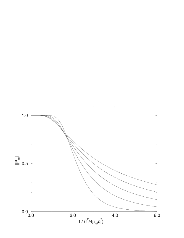
FIG. 1.: The weight $||P_{\text{rel}}||$ of the diffusion function outside the central singularity as a function of time for temperatures $k_{B}T/q^{2}=0.05,0.1,0.15,0.2,0.25$ (the steepest curve corresponds to $k_{B}T/q^{2}=0.05$). Time is measured in units of $r^{2}/4\mu_{\text{rel}}q^{2}$.

FIG. 2.: Double-logarithmic plot of the flux-noise power spectrum for a $c$ axis oriented Bi-2212 bulk single crystal at $T=84.2,84.5,84.6,84.7,85.2,85.7\mbox{ K}$ (from top to bottom). The critical temperature is $T_{c}=84.7\mbox{ K}$. The dashed line corresponds to the power law $S_{\phi}\propto\omega^{-3/2}$. Exemplary error bars are also shown.

FIG. 3.: The flux noise power for a $c$ axis oriented Bi-2212 crystal as a function of temperature at fixed frequency. The error bars from Monte-Carlo integration are also shown.

FIG. 4.: Log-log plot of the flux-noise power spectrum for a ultra-thin Bi-2212 film at $T=28,31,34\mbox{ K}$ (from top to bottom). The critical temperature if $T_{c}=31\mbox{ K}$. The dashed line corresponds to $S_{\phi}\propto\omega^{-3/2}$. Exemplary error bars are shown.

- [1] Present address: Indiana University, Dept. of Physics, Bloomington, IN 47405.
- [2] S. Scheidl and G. Hackenbroich, Europhys. Lett. 20, 511 (1992); B. Horovitz, Phys. Rev. B 47, 5947 (1993); G. Blatter, B.I. Ivlev, and H. Nordborg, Phys. Rev. B 48, 10 448 (1993); K.H. Fischer, Physica C 210, 179 (1993); S.W. Pierson, Phys. Rev. Lett. 73, 2496 (1994); M. Friesen, Phys. Rev. B 51, 632 (1995); S.W. Pierson, Phys. Rev. B 51, 6663 (1995); C. Timm, Phys. Rev. B 52, 9751 (1995).
- [3] V.L. Berezinskii, Zh. Eksp. Teor. Fiz. 61, 1144 (1971) [Sov. Phys. JETP 34, 610 (1972)]; J.M. Kosterlitz and D.J. Thouless, J. Phys. C 6, 1181 (1973); J.M. Kosterlitz, J. Phys. C 7, 1046 (1974).
- [4] B.I. Halperin and D.R. Nelson, J. Low Temp. Phys. 36, 599 (1979).
- [5] S.W. Pierson, Phys. Rev. Lett. 74, 2359 (1995).
- [6] P. Minnhagen and P. Olsson, Physica Scripta T42, 29 (1992).
- [7] C. Timm, Physica C 265, 31 (1996).
- [8] M.J. Ferrari, M. Johnson, F.C. Wellstood, J.J. Kingston, T.J. Shaw, and J. Clarke, J. Low Temp. Phys. 94, 15 (1994).
- [9] T.J. Shaw, M.J. Ferrari, L.L. Sohn, D.-H. Lee, M. Tinkham, and J. Clarke, Phys. Rev. Lett. 76, 2551 (1996).
- [10] C.T. Rogers, K.E. Myers, J.N. Eckstein, and I. Bozovic, Phys. Rev. Lett. 69, 160 (1992).
- [11] J. Appel, C. Timm, and A. Zabel, J. Low Temp. Phys. 99, 553 (1995).
- [12] C. Timm, Effects of Vortex Fluctuations in High-Temperature Superconductors, thesis, Universität Hamburg (Shaker, Aachen, 1996, ISBN 3-8265-1652-4).
- [13] V. Ambegaokar and S. Teitel, Phys. Rev. B 19, 1667 (1979); V. Ambegaokar, B.I. Halperin, D.R. Nelson, and E.D. Siggia, Phys. Rev. B 21, 1806 (1980).
- [14] J. Houlrik, A. Jonsson, and P. Minnhagen, Phys. Rev. B 50, 3953 (1994).
- [15] E. Domani, M. Schick, and R. Swendsen, Phys. Rev. Lett. 52, 1535 (1984).
- [16] P. Minnhagen, Rev. Mod. Phys. 59, 1001 (1987).
- [17] N.G. van Kampen, Stochastic Processes in Physics and Chemistry (North-Holland, Amsterdam, 1981).
- [18] B.I. Halperin, in Proceedings of Kyoto Summer Institute 1979—Physics of Low-Dimensional Systems, edited by Y. Nagaoka and S. Hikami (Publication Office, Prog. Theor. Phys., Kyoto), p. 53.
- [19] S.N. Artemenko and A.N. Kruglov, Phys. Lett. A 143, 485 (1990); M.V. Feigel’man, V.B. Geshkenbein, and A.I. Larkin, Physica C 167, 177 (1990); J.R. Clem, Phys. Rev. B 43, 7837 (1991).
- [20] M. Abramovitz and I. Stegun, Handbook of Mathematical Functions (Dover, New York, 1972).
- [21] J. Bardeen and M.J. Stephen, Phys. Rev. 140, A1197 (1965).
- [22] G. Blatter, M.V. Feigel’man, V.B. Geshkenbein, A.I. Larkin, and V.M. Vinokur, Rev. Mod. Phys. 66, 1125 (1994); C. de Morais Smith, B. Ivlev, and G. Blatter, Phys. Rev. B 52, 10 581 (1995).
- [23] A.T. Fiory, A.F. Hebard, P.M. Mankiewich, and R.E. Howard, Phys. Rev. Lett. 61, 1419 (1988); S.B. Ota, R.A. Rose, B. Jayaram, P.A.J. de Groot, and P.C. Lanchester, Physica C 157, 520 (1989); A. Gupta, P. Esquinazi, H.F. Braun, W. Gerhäuser, H.-W. Neumüller, K. Heine, and J. Tenbrink, Europhys. Lett. 10, 663 (1989).
- [24] D.S. Fisher, Phys. Rev. B 22, 1190 (1980).
- [25] A.M. Grishin, Y.M. Nikolaenko, A.V. Zinovuk, B.Y. Vengalis, and A. Flodström, Fiz. Nizk. Temp. 19, 42 (1993) [Low Temp. Phys. 19, 30 (1993)].
- [26] J.E. Mooij, in Percolation, Localization, and Superconductivity, edited by A.M. Goldman and S.A. Wolf (Plenum, New York, 1984), p. 325.
- [27] S. Martin, A.T. Fiory, R.M. Fleming, G.P. Espinosa, and A.S. Cooper, Phys. Rev. Lett. 62, 677 (1989).
- [28] R.F. Voss and J. Clarke, Phys. Rev. B 13, 556 (1976).