Coherent propagation of interacting particles in a random potential: the Mechanism of enhancement

Abstract

Coherent propagation of two interacting particles in $1d$ weak random potential is considered. An accurate estimate of the matrix element of interaction in the basis of localized states leads to mapping onto the relevant matrix model. This mapping allows to clarify the mechanism of enhancement of the localization length which turns out to be rather different from the one considered in the literature. Although the existence of enhancement is transparent, an analytical solution of the matrix model was found only for very short samples. For a more realistic situation numerical simulations were performed. The result of these simulations is consistent with

$\displaystyle l_{2}/l_{1}\sim l_{1}^{\gamma}\ \ ,$
where $l_{1}$ and $l_{2}$ are the single and two particle localization lengths and the exponent $\gamma$ depends on the strength of the interaction. In particular, in the limit of strong particle–particle interaction there is no enhancement of the coherent propagation at all ($l_{2}\approx l_{1}$).

I Introduction

The enhancement of the propagation length for two interacting particles (TIP) in a one-dimensional random potential was predicted in a paper by D. Shepelyansky [1] a couple of years ago. This result has attracted broad interest and stimulated active analytical [2, 7, 8, 9, 12] and numerical [3, 4, 5, 6, 10] investigations. 2-3-dimensional and quasi-$1d$ extensions of the model [1], as well as many other related problems have also been considered in various papers (see e.g. [2, 9, 11]). Moreover some of these new results may even be better established than the original one [1] (see also [13]).

More specifically, the first estimate [1] of the two-particle localization length was

$$l_{2}\sim l_{1}^{2}\ \ ,$$ (1)

where $l_{1}$ and $l_{2}$ are the one and two particle localization lengths.

Numerical simulations first of all have confirmed the existence of enhancement. As for the specific form of $l_{2}$, some authors [3] see deviations from (1), whereas others [5] report on the agreement with (1) (more concretely the authors of [5] agree with [1] in the $l_{1}$ dependence of $l_{2}$ although they still disagree in the overall normalization constant in (1)). However, the actual enhancement $l_{2}/l_{1}$ which was observed in numerical simulations, turns out to be rather small and varies from $l_{2}/l_{1}\sim 2$ in the first paper [1] to $l_{2}/l_{1}\sim 3-6$ for the most advanced computations [5].

We are going to consider particles moving in an exactly $1d$, weak, random potential. This means that the Anderson localization length $l_{1}$ is much larger than the de Broglie wave length $\lambda$ (for the Anderson hopping Hamiltonian (5) below $\lambda\sim 1$ and $l_{1}\gg 1$). Let the total length of the sample be $L\gg l_{1}$. The main achievement of [1] was the prediction of the existence of very unusual bound states for TIP (we will call them coherent states in order to distinguish from the usual molecular states [14]). The typical distance between particles for these new states is rather large, $x_{1}-x_{2}\sim l_{1}$, but the joint propagation length for two particles turns out to be even much larger $\Delta(x_{1}+x_{2})\sim l_{2}\gg l_{1}$. The total number of these new eigenstates is also sufficiently large: $\Delta N_{c}\sim(L/\lambda)(l_{1}/\lambda)$.

The central point for all the methods applied to calculation of the coherent propagation length $l_{2}$ was an estimate of the matrix element of the interaction in the basis of products of single particle localized states. However, as we will show in the following section, the estimate of the matrix element in ref. [1] crucially depends on the oversimplified assumption regarding the behavior of the single particle wave function and therefore is irrelevant. Surprisingly, all the authors of the following papers have accepted the matrix element estimate of [1] without any critical analysis.

This is why the main part of our paper will be devoted to an accurate estimate of the matrix element. This estimate allows us to perform mapping of the two-particle problem onto the physically relevant matrix model.

Surely the mapping itself is impossible without some (properly motivated) assumptions and order of magnitude estimates. Moreover, although we see a mechanism which should lead to the enhancement of the coherent propagation length, we have no rigorous proof that one could not find another source of enhancement. Therefore in the light of contradiction with existing predictions it should be very useful to find at least one new rigorous result. To this end we consider in Section 3 the strong coupling limit of the Shepelyansky model. It will be shown without any assumptions that for the very strong interaction between particles all the enhancement disappears and $l_{2}=l_{1}$. Thus the problem of two interacting particles exhibits some kind of duality between the parameters $U/t$ for weak ($U\ll t$) and $t/U$ for strong ($t\ll U$) coupling cases [15], where $U$ is the strength of interaction and $t$ is the typical single-particle energy (5,7). In both weak and strong coupling limits the enhancement disappears. As a function of $U$ the coherent propagation length $l_{2}$ should reach the maximum at some value of $U/t\sim 1$.

As we will show in the following section, the two main features of the matrix element of interaction lead us to associate the TIP problem with the matrix models which differs strongly from the previously considered ones [1, 7, 8, 9]. First of all it is the hidden hierarchy of the matrix elements. In general the matrix element of interaction in the basis of noninteracting two-particle states turns out to be much smaller than it was expected from the first estimate of ref. [1]. Only very small part of the matrix elements (namely $\sim 1/\sqrt{l_{1}}$) may exceed the original estimate by Shepelyansky [1]. This will be may be the most surprising result of our paper that such a few large matrix elements still may lead to a considerable enhancement. Another important feature of the matrix elements is the hidden order in their distribution. As we will show in Sections 5,6, after the proper ordering of the noninteracting basis the complicated hierarchy of the matrix elements may be described by the corresponding enveloping function of the relevant banded Gaussian random matrix model.

The matrix model we are going to consider turns out to be much more complicated than those investigated in [1, 3, 4, 5, 6, 7, 8, 10]. Therefore at first it would be useful to consider a simplified version of the problem. To this end in Section 5 we consider the TIP in the short sample with the total size $L$ being of the same order of magnitude as the single particle localization length $L\sim l_{1}$. In this case the corresponding random matrix is the so called Power-law Random Band Matrix (PRBM). The elements of this matrix decrease in a power-law fashion $M_{ij}\sim|i-j|^{-1}$ as one goes farther from the diagonal. Among the PRBM matrices of the general form with $M_{ij}\sim|i-j|^{-\alpha}$ those with $\alpha=1$ correspond to the phase transition from localized to delocalized regime [18]. For short sample we consider the so called inverse participation ratio $l_{ipr}$ (which is effectively the number of noninteracting two-particle states mixed into one chaotic eigenstate). The result reads

$$l_{ipr}\sim l_{1}^{\gamma_{ipr}}\ \ ,$$ (2)

where $\gamma_{ipr}$ is a function of the strength of the interaction approaching the value $\gamma_{ipr}=0$ in the weak and strong coupling limit. Equation (2) is proved analytically by the Renormalization Group method for $\gamma_{ipr}\ll 1$ but still for $\gamma_{ipr}\ln(l_{1})\gg 1$. The basic idea of calculating (2) follows the method of Levitov [17] who considered an even more complicated $3d$ problem. Numerical simulations also support the result (2) for $\gamma_{ipr}\sim 1$.

Unfortunately, for the realistic model with $L\gg l_{1}$ we could not find any convincing analytical solution (the matrix model itself will be described in Section 6). Nevertheless, we at least see that for a large sample the chaotic mixing of noninteracting two-particle states is systematically enhanced compared to a short sample. For example, it may be the same expression (2) for $l_{ipr}$ but with $\gamma^{\prime}>\gamma$. The perturbation theory for large $L$ may be used only if $\langle l_{ipr}\rangle-1\ll 1$. Nevertheless the physical expansion parameter for this perturbation theory still is $\ln(l_{1})U/t$ for the weak coupling and $\ln(l_{1})t/U$ for the strong coupling limit.

Therefore we have to perform numerical simulations for the matrix model associated with two particles on a large sample. The details of numerical procedure will be considered in Section 6 and now we will only make some general comments. The inverse participation ratio $l_{ipr}$ characterizes the complexity of the typical eigenstate in the Hilbert space formed by noninteracting two-particle states. On the other hand the coherent propagation length $l_{2}$ directly measures the spatial (lattice sites) dimension of the corresponding wave function. For practical calculations (Section 6) we define $l_{2}$ throw the mean squared size of the wave packet in longitudinal direction. We present our final result in the form

$$l_{2}/l_{1}\sim l_{1}^{\gamma}\ \ .$$ (3)

First of all, we definitely see that the exponent $\gamma$ is a function of the strength of interaction. Unfortunately we do not know too much about this dependence of $\gamma$ on $U$. The only claim we can make is that $\gamma$ should go to zero for the weak ($U\ll t$) and strong ($t\ll U$) coupling limiting cases (see also [19]). For arbitrary $U\sim t$ we expect $\gamma\sim 1$. For the concrete choice of parameters which we have considered numerically it was also $\gamma<1$. However, we do not know whether the same inequality $\gamma<1$ holds for any strength of interaction. Also for $l_{1}\gg\lambda$ the exponent $\gamma$ in (3) does not depend strongly on the strength of disorder or, in other words, $\gamma$ does not depend on $l_{1}$. The two-particle localization length of the form (3) with $\gamma<1$ was found also numerically in [3] by the transfer matrix method.

Of course the expression (3) (as well as (2)) should be used only for large $l_{1}$. This means that if one tries to extend (3) to small $l_{1}$, $\gamma$ will become a function of $l_{1}$ as well. For example, in order to fit the results of simulations, we use $\gamma=\gamma_{0}+c/l_{1}$. Our data (see figs. 2,3 below) shows that at least for the coherent propagation length $l_{2}$ the value of $\gamma$ does not vary strongly with $l_{1}$ . However, our numerical accuracy still is not enough to exclude completely some exotic dependence of $\gamma$ on $l_{1}$ for large $l_{1}$, say $\gamma=a+b\ln(l_{1})$ .

This paper is organized as follows. In Section 2 we give a general formulation of the problem and make a rough estimate of the matrix element of the interaction. It is shown by considering the modified Thouless block picture [20, 2] that effectively the interaction between particles is enhanced by a factor $\sim\ln(l_{1})$. In principle the material of Section 2 allows one to perform the mapping onto the matrix model which is done in Sections 5,6. However, in the next two sections we try to build a more stable foundation for this mapping. In Section 3 we consider the strong coupling limit of the Shepelyansky model. This consideration provides us with a better understanding as to how to distinguish regular and chaotic effects due to inter-particle interaction. On the other hand, the exact solution of the two-particle problem in the strong coupling regime allows us to perform the critical revision of the existing estimates of the coherent propagation length. In Section 4 we present a more rigorous estimate of the interaction matrix element than the one in Section 2. By averaging over the disordered potential in the “unimportant” part of its Fourier spectrum, which is not responsible for the global features of the localized single-particle states, we get rid of the problem of rapid oscillations in the matrix element. In Section 5 we investigate the effect of interaction in the short sample. Within the Renormalization Group approach of [17] a nontrivial solution of the model is found analytically at least for the weak effective interaction case. Finally, in the last Section 6 we describe the mapping of our coherent propagation problem onto the eigenvalue problem for some special Random Band Matrices. Features of this last model are investigated numerically.

II Formulation of the problem and preliminary estimates

Following [1] consider two particles on a $1d$ lattice with the Hamiltonian

$$H_{tot}=H(n_{1})+H(n_{2})+V_{int}\ \ .$$ (4)

There are no serious contradictions against considering the same problem in continuous $1d$-space. The Anderson lattice Hamiltonian, which is used traditionally, only simplifies the numerical calculations. The single particle Hamiltonian has the following nonzero elements for transitions between $n$-th and $m$-th sites of the lattice

$$H_{nm}=-t(\delta_{n,m+1}+\delta_{n,m-1})+w_{n}\delta_{n,m}\ \ .$$ (5)

Here $w_{n}$ is the random Gaussian potential and we suppose that the disorder is weak compared to the kinetic energy:

$$\overline{w_{n}w_{m}}\equiv w^{2}\delta_{nm}\ \ \ ,\ \ \ w\ll t\ \ .$$ (6)

In many papers devoted to the TIP delocalization problem the disordered potential is usually chosen to be uniformly distributed within the range $-W/2<w_{n}<W/2$ . The comparison with our results in this case may be made via trivial replacement $w^{2}=W^{2}/12$ . The Hubbard on-site interaction is defined as

$$\bigl{(}V_{int}\psi\bigr{)}_{n_{1},n_{2}}=U\delta_{n_{1},n_{2}}\psi(n_{1},n_{2})\ \ .$$ (7)

In general we assume that the interaction strength $U$ is of the same order of magnitude as the hopping matrix element $t$, though the more or less clear analytical results may be obtained only in the weak $(U\ll t)$ and strong $(U\gg t)$ coupling limits.

For simplicity we consider distinguishable particles, but all our results are equally valid for bosons or fermions with opposite spins.

The Anderson localization length has the form [21]

$$l_{1}=2\frac{4t^{2}-\epsilon^{2}}{w^{2}}\ \ ,$$ (8)

where $\epsilon$ is the single particle energy ($-2t<\epsilon<2t$). We will not be interested in the edges of the energy zone. Therefore for our purposes it will be enough to remember that $l_{1}\approx(t/w)^{2}$. For the lattice model (4,5) both $l_{1}$ and $l_{2}$ are naturally dimensionless.

An important feature of the single particle Hamiltonian (5), which was completely ignored in [1], is that due to the weakness of disorder it almost conserves the momentum. It is natural to parameterize the single particle energy $\epsilon$ by the momentum $k$ (again we are not interested in the very edges of the spectrum)

$$\epsilon=-2t\cos k\ \ .$$ (9)

Because of $w\ll t$, the eigenfunction of (5) $\psi_{\epsilon}(n)$ should be a linear combination of $\cos(k_{\epsilon}n)$ and $\sin(k_{\epsilon}n)$ with slowly varying amplitudes within the intervals small compared to $l_{1}$ (8). Therefore, it is convenient to consider the plane wave basis

$$\psi_{\epsilon}(n)=\sum_{k}C(k)|k\rangle\ \ ,\ \ |k\rangle=\frac{1}{\sqrt{L}}e^{ikn}\ \ ,$$ (10)

where $L$ is the total size of the sample $(L\gg l_{1})$. Now the amplitude $C(k)$ has two narrow peaks $(\Delta k\sim 1/l_{1})$ around $k=\pm k_{\epsilon}$.

Being the Fourier transform of the localized oscillating function $\psi_{\epsilon}(n)$, the amplitude $C(k)$ should manifest some simple features. Let the function $\psi_{\epsilon}(n)$ be localized around $n=n_{0}$ . Then one has

$$C({-k})=C({k})^{*}\$$ , (11)

$$C({k})=e^{ikn_{0}}\tilde{C}(k)\$$ , (12)

$$\tilde{C}(k)=f((k-k_{\epsilon})l_{1})\$$ , (13)

where $f(x)$ is some smooth function concentrated around the region $|x|\sim 1$.

The ensemble averaged value of $|C(k)|^{2}$ may be also extracted from the textbook [16]

$$\langle|C(k)|^{2}\rangle\sim\left[(\epsilon-\epsilon_{\scriptscriptstyle k})^{2}+\left(\frac{1}{l_{1}}\frac{d\epsilon}{dk}\right)^{2}\right]^{-1}\ \ ,$$ (14)

where $l_{1}$ is the Anderson localization length (8). This is the averaged value of $|C(k)|^{2}$ and therefore it can not be used directly for our following calculations. However, (14) gives the proper estimate of the amplitude of the wave function in the momentum representation $C(k)$ in the whole range of variation of the momentum $k$.

In order to illustrate the physical origin of (14) it is useful to rewrite the single particle Schrödinger equation in the plane wave basis:

$$C(k)=\sum_{q}\frac{\langle k|\hat{w}|q\rangle}{\epsilon-\epsilon_{\scriptscriptstyle k}}C(q)\ \ \ ,$$ (15)

where by $\hat{w}$ we have denoted the random potential (5) and $\epsilon$ is the single particle energy corresponding to this eigenfunction. In general this equation is not easier to solve than the original Schrödinger equation with the Anderson Hamiltonian (5). However, in order to extract the information we need, it is enough to observe, that the r.h.s. of (15) is saturated by the only $C(q)$ with $q-k_{0}\sim 1/l_{1}$, and (for negative $q$) $q+k_{0}\sim 1/l_{1}$ , where $k_{0}$ is the first positive solution of the equation $\epsilon_{0}=-2t\cos k_{0}$ . Therefore, far away from the region $|k\pm k_{0}|\sim 1/l_{1}$ the amplitude of $C(k)$ is determined by the energy denominator in (15) in accordance with (14).

Now it is easy to write down the estimate for the amplitudes $C(k)$.

$$C(k)\sim\sqrt{\frac{l_{1}}{L}}\ \ \ {\rm if}\ \ \ k\pm k_{\scriptscriptstyle 0}\sim 1/l_{1}\ \ ,$$ (16)

$$C(k)\sim\sqrt{\frac{l_{1}}{L}}\frac{1}{(k_{\scriptscriptstyle 0}\pm k)l_{1}}\ \ \ {\rm if}\ \ \ 1/l_{1}\ll|k{\scriptscriptstyle 0}\pm k|\ll 1\ \ .$$ (17)

Everywhere except the Section 5 we suppose that $L\gg l_{1}$. The formula (16) follows directly from the normalization condition $\sum|C(k)|^{2}=1$. The denominator $k_{\scriptscriptstyle 0}\pm k$ in (17) stands for $\epsilon-\epsilon_{\scriptscriptstyle k}$ in (15) and all the other factors may be found by comparison of (17) with (16) at $|k\pm k_{\scriptscriptstyle 0}|\sim 1/l_{1}$. In general, for arbitrary $|k\pm k_{\scriptscriptstyle 0}|\sim 1$

$$C(k)\sim\sqrt{\frac{1}{l_{1}L}}\ \ \ .$$ (18)

Now let us take into account the interaction $V_{int}$ . It is natural to use the basis of products of single particle localized states

$$|1,2\rangle=\psi_{1}(n_{1})\psi_{2}(n_{2})\ \ \ .$$ (19)

This wave function describes distinguishable particles. The generalization to the case of bosons or electrons with opposite spins is straightforward. Moreover, in the following section we will effectively turn to the bosonic case because the Hubbard short-range interaction (7) separates the symmetric and antisymmetric eigenstates and the Hamiltonian (4) is invariant under particle permutation ($n_{1}\rightarrow n_{2}\ ,\ n_{2}\rightarrow n_{1}$).

In terms of the summation over the original lattice-sites the matrix element between the states (19) takes the form

$$\langle 3,4|V_{int}|1,2\rangle=U\sum_{n}\psi_{1}(n)\psi_{2}(n)\psi_{3}(n)\psi_{4}(n)\ \ .$$ (20)

Each wave function here decays exponentially outside the segment of the lattice of length $\sim l_{1}$. Therefore the matrix element (20) vanishes if not all the functions $\psi_{i}(n)$ overlap. Everywhere in the following we consider only the matrix elements for overlapping states.

In order to estimate the matrix element (20), the author of [1] assumed that each wave function $\psi_{i}(n)$ within its segment $\sim l_{1}$ is completely random. Under this assumption one immediately finds the following estimate

$$\langle 3,4|V_{int}|1,2\rangle_{chaotic}\sim\frac{U}{l_{1}^{3/2}}\ \ .$$ (21)

On the other hand, the assumption itself about chaoticity of the wave function is evidently inconsistent with the accurate estimate of the Fourier transform (14) - (18).

The difficulties in estimation of the matrix element (20) originate from the almost regular and fast oscillations of the single particle wave functions. It may be seen immediately from any toy example, that the matrix element for oscillating functions is usually much more suppressed than for random ones. On the other hand, for oscillating wave functions it is natural to consider the matrix element (20) in terms of plane wave amplitudes (10)

$$\langle 3,4|V_{int}|1,2\rangle=\frac{U}{L}\sum_{k_{i}}C_{3}^{\star}({k_{\scriptscriptstyle 3}})C_{4}^{\star}({k_{\scriptscriptstyle 4}})C_{1}({k_{\scriptscriptstyle 1}})C_{2}({k_{\scriptscriptstyle 2}})\delta_{k_{1}+k_{2},k_{3}+k_{4}}\ \ .$$ (22)

Here the $\delta$-function accounts for the conservation of the total momentum by the interaction $V_{int}$. One may use (11) in order to demonstrate in terms of $C(k)$ that only the matrix elements between spatially overlapping states $\psi_{1},\ \psi_{2},\ \psi_{3},\ \psi_{4}$ survive.

Equation (22) together with the plane wave amplitudes (16)-(18) is enough for the rough estimate of the matrix element of $V_{int}$. As we have said, we will consider only the overlapping states ($n_{0_{i}}-n_{0_{j}}\sim l_{1}$ (11)), otherwise the matrix elements decay exponentially. We have considered three different estimates (16), (17), and (18) of the plane wave amplitude $C(k)$ for different ranges of variation of the momentum $k$. Correspondingly, now we are going to present the three different estimates of the matrix element (22). First of all, consider the single particle states $|1\rangle,|2\rangle,|3\rangle,|4\rangle$ for which the momentum is almost conserved in the transition (22). This means that $k_{\scriptscriptstyle 0_{1}}+k_{\scriptscriptstyle 0_{2}}\approx k_{\scriptscriptstyle 0_{3}}+k_{\scriptscriptstyle 0_{4}}$ (the momentum $k_{\scriptscriptstyle 0}$ is connected with the single particle energy via (9)). As we know each function $C_{i}(k)$ consists of two narrow ($\Delta k\sim l_{1}^{-1}$) peaks. Just for $k_{\scriptscriptstyle 0_{1}}+k_{\scriptscriptstyle 0_{2}}\approx k_{\scriptscriptstyle 0_{3}}+k_{\scriptscriptstyle 0_{4}}$ all this peaks overlap and therefore

$$k_{\scriptscriptstyle 0_{1}}+k_{\scriptscriptstyle 0_{2}}-k_{\scriptscriptstyle 0_{3}}-k_{\scriptscriptstyle 0_{4}} \sim 1/l_{1}\ \ ,$$ (23)

$$\langle 34|V_{int}|12\rangle\sim\frac{U}{L}\left(\frac{l_{1}}{L}\right)^{2}\left(\frac{L}{l_{1}}\right)^{3} \sim \frac{U}{l_{1}}\ \ .$$ (24)

Here the first factor $U/L$ comes directly from (22), $(l_{1}/L)^{2}$ is the fourth power of the wave function at the maximum (16), and $(L/l_{1})^{3}$ is the effective number of terms in the sum in (22). Suppose now that the momentum conservation is completely violated $\Delta k\sim 1$. In this case the peaks for all $C(k)$ could not overlap simultaneously. One of the functions should be taken at the tail (18):

$$k_{\scriptscriptstyle 0_{1}}+k_{\scriptscriptstyle 0_{2}}-k_{\scriptscriptstyle 0_{3}}-k_{\scriptscriptstyle 0_{4}} \sim 1\ \ ,$$ (25)

$$\langle 34|V_{int}|12\rangle\sim\frac{U}{L}\left(\frac{l_{1}}{L}\right)^{2}\frac{4}{l_{1}}\left(\frac{L}{l_{1}}\right)^{3} \sim \frac{U}{l_{1}^{2}}\ \ .$$ (26)

Here compared to (23) we have replaced one of the plane wave amplitudes (16) by (18). The factor $4$ in (25) should not be considered very seriously, it simply symbolizes that this replacement may be done in $4$ ways.

Finally, the most interesting case is if the momentum difference $\Delta k=k_{\scriptscriptstyle 0_{1}}+k_{\scriptscriptstyle 0_{2}}-k_{\scriptscriptstyle 0_{3}}-k_{\scriptscriptstyle 0_{4}}$ is much larger than $1/l_{1}$ but still is small compared to $1$. To be more accurate one should define a few $\Delta k$-s , $\Delta k=\pm k_{\scriptscriptstyle 0_{1}}\pm k_{\scriptscriptstyle 0_{2}}\pm k_{\scriptscriptstyle 0_{3}}\pm k_{\scriptscriptstyle 0_{4}}$. The matrix element will be enhanced as in (27) below if at least one $\Delta k$ is much smaller than $1$. We leave the consideration of this complication until Section 4. The formula (17) for the “short range tail” now allows one to find the following estimate

$$1/l_{1} \ll |k_{\scriptscriptstyle 0_{1}}+k_{\scriptscriptstyle 0_{2}}-k_{\scriptscriptstyle 0_{3}}-k_{\scriptscriptstyle 0_{4}}|\ll 1\ \ ,$$ (27)

$$\langle 3,4|V_{int}|1,2\rangle \sim \frac{U}{l_{1}^{2}}\frac{1}{k_{\scriptscriptstyle 0_{1}}+k_{\scriptscriptstyle 0_{2}}-k_{\scriptscriptstyle 0_{3}}-k_{\scriptscriptstyle 0_{4}}}\ \ .$$ (28)

Just this last matrix element will lead to the enhancement of the two-particle localization length. We will return to the more accurate and detailed estimate of the matrix element for the case (27) in Section 4.

Note that all these estimates (23),(25),(27) differ from those of [1] $\langle 3,4|V_{int}|1,2\rangle\sim U/l_{1}^{3/2}$ (21).

The natural tool for the investigating the coherent propagation proposed in [2] is the Thouless block picture [20]. Consider the two one-particle $1d$ Hamiltonians with the interaction (4) as the $2d$-Hamiltonian on a large $L\times L$ square. Because the Hubbard interaction (7) affects only the diagonal $n_{1}=n_{2}$ it is natural to use (for a moment) the center of mass variables $\frac{1}{2}(n_{1}+n_{2})$ and $(n_{1}-n_{2})$. Now the large $2d$ system should be mentally divided into square blocks of size $l_{b}\times l_{b}$ with $l_{b}\sim l_{1}$. Due to the exponential decay of the localized eigenstates at $|n-n_{0}|>l_{1}$ and the diagonal form of the interaction (7), it is enough to consider only one row of blocks with $|n_{1}-n_{2}|<l_{b}/2$. Thus our $2d$-system reduces to quasi-$1d$ one. The $m$-th block is defined by the inequalities

$$|n_{1}-n_{2}|<\frac{l_{b}}{2}\ \ ,$$ (29)

$$ml_{b}<\frac{n_{1}+n_{2}}{2}<(m+1)l_{b}\ \ .$$ (30)

About $l_{b}^{2}\sim l_{1}^{2}$ states (19) fall down into each block. Thus the typical level separation within one block is $\Delta\sim t/l_{1}^{2}$. We suppose that the interaction (7) mixes the states from the same block and with about the same amplitude the states from the nearest blocks. If one believes in the estimate (21) [1] the delocalization (enhancement of the coherent propagation length) follows immediately from the inequality [2]

$$\langle 3,4|V_{int}|1,2\rangle_{chaotic}\sim\Delta\sqrt{l_{1}}\gg\Delta\ \ .$$ (31)

However, unfortunately the matrix element (21) is inconsistent with the correct estimate.

Consider now, what one can conclude from the correct estimates (23)-(27)? In order to understand whether the enhancement exists or not, it is enough to fix one state (19) belonging, say to the $m$-th block and to estimate the number of other states mixed to that one with amplitude $\sim 1$. First of all, consider the largest matrix element (23). This matrix element $\langle 34|V_{int}|12\rangle\sim 1/l_{1}$ is $l_{1}$ times larger than the typical level spacing within one block. Nevertheless, the momentum conservation necessary for (23) reduces in the same $l_{1}$ times the number of states in one block available for this transition. Thus

$$\Delta_{eff_{0}}\sim\langle 3,4|V_{int}|1,2\rangle\sim\frac{1}{l_{1}}\ \ \ {\rm for}\ \ \ |k_{\scriptscriptstyle 0_{1}}+k_{\scriptscriptstyle 0_{2}}-k_{\scriptscriptstyle 0_{3}}-k_{\scriptscriptstyle 0_{4}}|<\frac{1}{l_{1}}\ \ ,$$ (32)

which means that about one state is strongly mixed to the given one by this matrix element.

So we are looking for the admixture to the state $|1,2\rangle$ belonging to the $m$-th block. Let us divide all the $\sim l_{1}^{2}$ states $|3,4\rangle$ from the $m$-th and two nearest blocks into smaller portions in accordance with the momentum non-conservation $\Delta k=k_{\scriptscriptstyle 0_{1}}+k_{\scriptscriptstyle 0_{2}}-k_{\scriptscriptstyle 0_{3}}-k_{\scriptscriptstyle 0_{4}}$. Into the $n$-th portion we will put the states with $2^{n}/l_{1}<|\Delta k|<2^{n+1}/l_{1}$. Due to (27) one may easily compare the effective level splitting $\Delta_{eff_{n}}$ for each portion with the corresponding matrix element

$$\Delta_{eff_{1}}\sim\langle 3,4|V_{int}|1,2\rangle\sim\frac{1}{2}\frac{1}{l_{1}}\ \ \ {\rm for}\ \ \ \frac{1}{l_{1}}<|k_{\scriptscriptstyle 0_{1}}+k_{\scriptscriptstyle 0_{2}}-k_{\scriptscriptstyle 0_{3}}-k_{\scriptscriptstyle 0_{4}}|<\frac{2}{l_{1}}\ \ ,$$ (33)

$$\Delta_{eff_{2}}\sim\langle 3,4|V_{int}|1,2\rangle\sim\frac{1}{4}\frac{1}{l_{1}}\ \ \ {\rm for}\ \ \ \frac{2}{l_{1}}<|k_{\scriptscriptstyle 0_{1}}+k_{\scriptscriptstyle 0_{2}}-k_{\scriptscriptstyle 0_{3}}-k_{\scriptscriptstyle 0_{4}}|<\frac{4}{l_{1}}\ \ ,$$ (34)

$$\ \ \ \ \ \ \ \ \ \ .\,.\,.\,.\,.\,.\,.\,.\,.\,.\,.\,.\,.\,.\,.\,.\,.\,.\,.\,.\,.\,.$$ (35)

$$\ \ \ \ \ \ \ \ \ \ .\,.\,.\,.\,.\,.\,.\,.\,.\,.\,.\,.\,.\,.\,.\,.\,.\,.\,.\,.\,.\,.$$ (36)

$$\Delta_{eff_{n}}\sim\langle 3,4|V_{int}|1,2\rangle\sim\frac{1}{2^{n}}\frac{1}{l_{1}}\ \ \ {\rm for}\ \ \ \frac{2^{n-1}}{l_{1}}<|k_{\scriptscriptstyle 0_{1}}+k_{\scriptscriptstyle 0_{2}}-k_{\scriptscriptstyle 0_{3}}-k_{\scriptscriptstyle 0_{4}}|<\frac{2^{n}}{l_{1}}\ \ .$$ (37)

The number of states falling into the $n$-th portion increases like $2^{n}$, but simultaneously the matrix element (27) decreases by the same factor. The number of rows in the formula (33) is evidently $\ln(l_{1})$ and therefore we see that each simple state $|1,2\rangle$ (19) may be mixed with $\sim\ln(l_{1})\gg 1$ others.

We will see in the Sections 5,6 how this $\sim\ln(l_{1})$ enhancement may lead to the coherent propagation length (2,3)

The approach of ref. [12] is sometimes considered as one which allows to get the better understanding of the TIP-problem. Therefore before going further we would like to consider the validity of the method of [12] in the light of our estimate for the two-particle matrix element (23)-(27).

The authors ref.[12] calculated the averaged Breit-Wigner width $\Gamma$ for TIP in small $L\ll l_{1}$ sample. Connection with the full TIP problem is made via the relation

$$l_{2}/l_{1}\sim\Gamma\rho\ \ ,$$ (38)

where $\Gamma$ is the Breit-Wigner width for the sample of the size $L\sim l_{1}$ and $\rho$ is the total density of two-particle states in the same sample. The authors do not derive the eq. (38), but find the support for it in the refs. [1, 2, 6, 7, 8]. The eq. (38) seems to be useful if the interaction would be able to mix with about the same probability all overlapping two-particle states. However, as we have shown in (23,25,27) the actual matrix elements between different states are of the very different magnitude. For example the total width $\Gamma$ in (38) is determined by a very small fraction $\sim 1/l_{1}$ of all two-particle states. In its turn the main part of the density of states $\rho$ is given by the states which may be mixed only by a very small matrix element (25) (in $1/\sqrt{l_{1}}$ times smaller than is needed for the estimate of ref. [1]).

Thus, there seems to be no reason to join in one expression (38) the $\Gamma$ and $\rho$ which have so different physical origin. One may divide all the two-particle states into a classes so that the matrix elements from the given state $|12\rangle$ to any other within one class will be of the same order of magnitude. Just as we did in the eq. (33). Now the natural generalization of (38) will be to introduce the large parameter (see (33))

$$g\sim\sum_{classes}\Gamma_{i}\rho_{i}\sim U/t\ln(l_{1})\ \ ,$$ (39)

where $\Gamma_{i}$ is the partial width for the state $|12\rangle$ to decay into the $i$-th class and $\rho_{i}$ is the density of states in this class. This $g$ will work as the effective expansion parameter in the perturbative treatment of the TIP problem. It is however still a long way from eq. (39) to the accurate estimate of the coherent propagation length $l_{2}$. This will be just the main aim of our Sections 5,6 to show that in order to find the TIP coherent propagation length one should most naturally exponentiate $g$ and that $l_{2}/l_{1}\sim\exp(const\times g)$ .

III The strong coupling limit

The existing attempts to reduce the two particle problem to a random matrix one were all based on the assumption that the mixing of the simple states (19) due to the particle–particle interaction is sufficiently random.

On the other hand, if there is no disorder ($w_{n}=0$) the exact eigenfunctions of the Hamiltonian (4) are easy to found in terms of the variables $n_{1}-n_{2}$ and $n_{1}+n_{2}$ . Among these solutions the eigenfunctions decaying exponentially at large $|n_{1}-n_{2}|$ form the molecular bound states sub-band. All remaining wave functions from the continuous spectrum will be formed by rather regular combinations of $\sin(n_{1,2})$ and $\cos(n_{1,2})$, though having a finite kink at $n_{1}=n_{2}$ . Thus for $w_{n}\equiv 0$ the particle–particle interaction leads to considerable but rather regular rearrangement of the noninteracting product basis set (19). It is evident that for finite but small disorder ($|w_{n}|\ll t$) the regular modification of the wave–functions should survive, at least in some sense.

This regular rearrangement of the noninteracting basis may be thought as the mixing of each state (19) with many others via the largest matrix elements (23). The energy denominator for this many states in general is not small (up to $\Delta E\sim t$) and thus each individual admixture is added to (19) with a rather small amplitude. However, due to the large number of these effectively regular contributions, the final change of the wave function may be of the order of one.

Thus we divide (although slightly arbitrarily) all the admixtures to the given state $|1,2\rangle$ into two classes. First, those with small energy denominator $\Delta E<1/l_{1}$. These contribution are completely random as we show in the following section and lead to the large coherent propagation length.

The second type of admixtures are those with large energy denominator $\Delta E>1/l_{1}$. We see no mechanism, how these corrections may lead to the enhancement of the propagation length (although also we have no rigorous proof that such mechanism does not exist). Moreover, we are going to show in this section that these regular effects in the strong coupling limit should lead to the suppression of the two particle propagation. Up to now the authors of all the papers devoted to the TIP problem have examined only the monotonous dependence of $l_{2}$ on $U$ (say $l_{2}\sim U^{2}$ in [1] and $l_{2}\sim|U|$ in [5]). Among other papers the numerical result of ref. [5] may be considered as the most serious objection to our prediction (3). However, our main statement in this section is that all quantities characterizing the TIP problem should depend in some complicated way on $U/t$ even for $U\sim t$. For example $\gamma$ in (3) for $U<t$ may be of the form (we do not worry now about the sign of $U$)

$$\gamma(U)=\gamma_{1}\frac{U}{t}+\gamma_{2}\left(\frac{U}{t}\right)^{2}+\gamma_{3}\left(\frac{U}{t}\right)^{3}+...\ \ ,$$ (40)

where all $\gamma_{1},\gamma_{2},\ ...$ are of the order of one $\gamma_{i}\sim 1$. The same holds for the overall normalization of (3). Therefore, because the authors of [5] have not taken into account this complicated dependence of $l_{2}$ on $U$, we believe that they have used the irrelevant fitting function for the $l_{1}$ dependence as well (see also the discussion [19]).

Let us consider now the case of very strong Hubbard interaction (7) $U\gg t$. Consider also the new basis set of states relevant to this limiting case. First of all, the trivial subset of diagonal states evidently decouples for the large $U$

$$|n\rangle=\delta_{n,n_{1}}\delta_{n,n_{2}}\ \ ,$$ (41)

where $n_{1},n_{2}$ are the lattice variables for two particles. These states form a narrow molecular zone with energy close to $U$ and the effective molecule mass close to $\sim U/t^{2}$. If $t^{2}/U\ll w$ these particles do not move. If $t^{2}/U\gg w$, Anderson localization takes place, though the localization length is small compared to (8).

The most surprising fact is that in the model under consideration all the remaining eigenstates in the strong coupling limit may be found exactly. Let $\psi_{i}(n)$ be a set of localized single particle states. Then it is easy to construct the set of antisymmetric states

$$|1,2\rangle^{A}=\frac{1}{\sqrt{2}}[\psi_{1}(n_{1})\psi_{2}(n_{2})-\psi_{2}(n_{1})\psi_{1}(n_{2})]\,\,\,\,\,\,,$$ (42)

which are obviously the exact eigenfunctions of the Hamiltonian (4) even for arbitrary $U$. In addition to (41) and (42) let us consider the symmetric functions

$$|1,2\rangle^{S}=\frac{1}{\sqrt{2}}sign(n_{1}-n_{2})\big{[}\psi_{1}(n_{1})\psi_{2}(n_{2})-\psi_{2}(n_{1})\psi_{1}(n_{2})\big{]}\ \ ,$$ (43)

where $sign(x)=x/|x|$ and $sign(0)=0$. First of all, the states (41)-(43) form the complete orthogonal set and are all localized. Any two vectors from (41) and (42) are orthogonal by construction. The states (43) are evidently orthogonal to (42) and (41). Finally, the integral of the product of any two symmetric states (43) coincides with the one for corresponding antisymmetric states. Therefore, (41)-(43) may be used as a new basis instead of (19). Moreover, as we will show now the symmetric functions (43) are also the exact eigenfunctions of (4) for $U\rightarrow\infty$ (or $U\gg t$).

The physical explanation, why (43) are the exact eigenfunctions for large $U$ is almost trivial. Consider our two particles in $1d$ as one particle on a $2d$ square $L\times L$. For infinite $U$ this particle simply could not penetrate through the barrier (7) along the diagonal of the square. As we said before, the antisymmetric states (42) are by construction the exact solutions. But now, because the two parts of the volume are separated by an opaque barrier, the symmetric states (43), as well as any linear combination of (42) and (43), become exact eigenfunctions of the Hamiltonian (4).

However, this simple explanation does not allow one to find the corrections to (43) for large but finite $U$. Therefore below we calculate the matrix element of the effective interaction between the two states $|1,2\rangle^{S}$ and $|3,4\rangle^{S}$ for $U\gg t$. Consider the total Hamiltonian $H_{tot}$ (4) as a matrix in the basis (41)-(43). It is enough to consider only the symmetric states (41) and (43). The only surviving non-diagonal elements of this matrix are

$$\langle n|H_{tot}|1,2\rangle^{S}=-\sqrt{2}t\big{[}(\psi_{1}(n+1)-\psi_{1}(n-1))\psi_{2}(n)-(\psi_{2}(n+1)-\psi_{2}(n-1))\psi_{1}(n)\big{]}\ .$$ (44)

Besides that there are evidently only the diagonal elements

$$\langle n|H_{tot}|n\rangle=U+w_{n}\approx U\ \$$ , (45)

$$\langle 3,4|^{S}\,H_{tot}|1,2\rangle^{S}=\epsilon_{\scriptscriptstyle 1}+\epsilon_{\scriptscriptstyle 2}\ \$$ . (46)

Thus the mixing of the two states $|1,2\rangle^{S}$ and $|3,4\rangle^{S}$ may appear only in the second order of perturbation theory. Consider for simplicity the case $\epsilon_{\scriptscriptstyle 1}+\epsilon_{\scriptscriptstyle 2}\approx\epsilon_{\scriptscriptstyle 3}+\epsilon_{\scriptscriptstyle 4}$ . The simple perturbative calculation immediately leads to the effective interaction

$$\langle 3,4|^{S}\,U_{eff}|1,2\rangle^{S}=\sum_{n}\frac{\langle 3,4|^{S}\,H_{tot}|n\rangle\langle n|H_{tot}|1,2\rangle^{S}}{U-\epsilon_{\scriptscriptstyle 1}-\epsilon_{\scriptscriptstyle 2}}=\frac{2t^{2}}{U-\epsilon_{\scriptscriptstyle 1}-\epsilon_{\scriptscriptstyle 2}}\frac{4}{L}$$ (47)

$$\times\sum_{k_{1}+k_{2}=k_{3}+k_{4}}C_{1}(k_{\scriptscriptstyle 1})C_{2}(k_{\scriptscriptstyle 2})C_{3}^{\star}(k_{\scriptscriptstyle 3})C_{4}^{\star}(k_{\scriptscriptstyle 4})[\sin k_{\scriptscriptstyle 3}-\sin k_{\scriptscriptstyle 4}][\sin k_{\scriptscriptstyle 1}-\sin k_{\scriptscriptstyle 2}]\ .$$ (48)

This effective matrix element should be compared with (22). First of all we see that the strength of the interaction $U$ has been replaced by $t^{2}/U$. Thus the corrections to (43) are of the order of $t/U\ll 1$. In particular the estimate of the matrix element (23-27) evidently holds for (47) up to the trivial replacement $U\rightarrow t^{2}/U$ (see also (84) below).

Another important difference between (22) and (47) are the $\sin(k_{i})$-s, which can not lead to any enhancement and even tends to suppress the matrix element for $\epsilon_{\scriptscriptstyle 1}\approx\epsilon_{\scriptscriptstyle 2}$ and $\epsilon_{\scriptscriptstyle 3}\approx\epsilon_{\scriptscriptstyle 4}$ .

Thus we see that the problem of TIP should be treated within the two sufficiently different (somehow dual) approaches in the weak (20,22) and strong (47) interaction cases. However the $l_{1}$ dependence of the matrix element estimated in (23-27) coincides for both limits.

In the intermediate region $U\sim t$ both formulas (22) and (47) should be modified. In order to illustrate the nature of this modification consider for example the case $U<t$. Let us consider also the eigenstates with the two-particle energy close to some value $E_{0}$. It is convenient to consider the narrow strip in energy of the width $2\delta_{E}\sim t/l_{1}$ around $E_{0}$. As we have told at the beginning of this section the states within the strip $|E_{ij}-E_{0}|<\delta_{E}$ will be mixed chaotically. The only role played by the other states $|E_{ij}-E_{0}|>\delta_{E}$ is to renormalize regularly the effective matrix element between chaotically mixed ones. Let the states $|1,2\rangle$ and $|3,4\rangle$ belong to the strip $|E_{12}-E_{0}|,|E_{34}-E_{0}|<\delta_{E}$ ($|1,2\rangle$ and $|3,4\rangle$ are the simple products of noninteracting localized single particle states). Than one may write perturbatively the renormalized interaction

$$\langle 3,4|\,V_{ren}|1,2\rangle = \langle 3,4|\,V_{int}|1,2\rangle+$$ (49)

$$+\sum_{|E_{ij}-E_{0}|>\delta_{E}}\frac{\langle 3,4|\,V_{int}|i,j\rangle\langle i,j|\,V_{int}|1,2\rangle}{E_{0}-E_{ij}}+...\ \ .$$ (50)

The most interesting for us situation is when the momentum in the transition $|1,2\rangle\rightarrow|3,4\rangle$ is not conserved and the leading contribution in (49) is described by (27). In this case one of the matrix elements in the sum in (49) may be large like $U/l_{1}$ (23) (and the small factor $1/l_{1}$ in it may be compensated due to a number of terms in the sum). However, as one may easily see, the second matrix element in the sum should again be of the form (27). Thus we see no reason, why the renormalization of the bare matrix element (20,22,27) will not be described by the series of the kind $1+(U/t)+(U/t)^{2}+...$ .

It is clear that the states (43) should be also the proper solutions for the continuous version of the model (4) with strong repulsive interaction $V_{int}=G\delta(x-y)$. Of course in this case the energy $\epsilon_{\scriptscriptstyle 1}+\epsilon_{\scriptscriptstyle 2}$ should be also sufficiently small ($\epsilon_{\scriptscriptstyle 1}+\epsilon_{\scriptscriptstyle 2}\ll G^{2}$). In fact the continuous model may be simply considered as the low energy limit of our lattice model (4).

To conclude this section let us say again that the comparison of our eq. (47) with (22) shows that the crossover from weak to strong coupling regime takes place somewhere at $U/t\sim 1$. The authors of refs. [5, 12] have mentioned that they would expect some deviations from their predictions at large $U$. However as we can understand, they have in mind just the case $|U|\gg t$. Moreover, one would even hardly found from [5, 12], what is the sign of these expected corrections.

IV Estimation of the matrix element

The rough estimate of the matrix element (27) in principle is enough to formulate the effective matrix model which will be considered in the following two sections. Nevertheless, because the distribution of the matrix elements is of crucial importance for our result, we would like to present in this section a more accurate estimate than (27). We will consider both the matrix element of the interaction potential (7) in the basis of the simple products of noninteracting single-particle states (19) and the matrix element of the effective interaction in the strong coupling case (47).

Although, our formulas (81),(82) below are too detailed to be used for the mapping onto the matrix model (Sections 5,6), they may be a good base for the comparison with the numerical experiment, say, of the kind mentioned in [3].

Our main problem is to make a reliable estimate of the matrix element with oscillating wave functions. As we have said in Section 2, we are mostly interested in the case when the four plane wave amplitudes $C_{i}(k)$ do not overlap strongly in the matrix element (22). This means that at least one of the wave functions should be taken at the tail (17). For this case the Schrödinger equation (15) may be further simplified

$$C(k)_{tail}=\sum_{|q-k_{0}|<\delta}\frac{\langle k|\hat{w}|q\rangle}{\epsilon-\epsilon_{\scriptscriptstyle k}}C(q)_{core}+\sum_{|q+k_{0}|<\delta}\frac{\langle k|\hat{w}|q\rangle}{\epsilon-\epsilon_{\scriptscriptstyle k}}C(q)_{core}\ \ \ ,$$ (51)

where $|k\pm k_{\scriptscriptstyle 0}|\gg 1/l_{1}$ and $\delta\sim 1/l_{1}$ (say $\delta=5/l_{1}$ ). Here we have divided each wave function $C(k)$ into two parts. One part is “the core”, or the largest part of the wave function coming from $|k-k_{\scriptscriptstyle 0}|<\delta$ and $|k+k_{\scriptscriptstyle 0}|<\delta$. Another part is the tail at $|k\pm k_{\scriptscriptstyle 0}|>\delta$ .

The matrix element of the random potential between the two plane waves which appeared in (51) is equal to

$$\langle k^{\prime}|\hat{w}|k\rangle\equiv\langle 0|\hat{w}|k-k^{\prime}\rangle={1\over{L}}\sum_{n=1}^{L}w_{n}e^{i(k-k^{\prime})n}.$$ (52)

For the quantitative calculation of the matrix element of the interaction potential it is important that (52) depends only on the one variable $k-k^{\prime}$. The distribution of $\langle k^{\prime}|\hat{w}|k\rangle$ is an usual normal one with variance (see (6))

$$\overline{|\langle k^{\prime}|\hat{w}|k\rangle|^{2}}=w^{2}/L.$$ (53)

Formula (51) allows us to demonstrate one important difference between the “core” and the “tail” of single particle wave function. The main part of the wave function is almost regular (one should not worry about the trivial randomness due to the position of the center of the wave packet $n_{0}$ (11) because we consider only overlapping functions). On the other hand the tail (51) due to $\langle 0|\hat{w}|k-k^{\prime}\rangle$ is sufficiently random. More accurately, $C(k)$ and $C(k^{\prime})$ are correlated only for $k-k^{\prime}\sim 1/l_{1}$ and are not correlated for $|k-k^{\prime}|\gg 1/l_{1}$.

This observation allows us to define a relatively simple procedure of averaging the squared matrix element (20),(22). The mathematically rigorous way of averaging the $|\langle 3,4|V_{int}|1,2\rangle|^{2}$ would be to introduce eight collective variables : centers of the wave packets $n_{\scriptscriptstyle 0_{1}},n_{\scriptscriptstyle 0_{2}},n_{\scriptscriptstyle 0_{3}},n_{\scriptscriptstyle 0_{4}}$ and the energies $\epsilon_{\scriptscriptstyle 1},\epsilon_{\scriptscriptstyle 2},\epsilon_{\scriptscriptstyle 3},\epsilon_{\scriptscriptstyle 4}$. The “rigorous” averaging should then be performed over the ensemble of random Hamiltonians (5) for fixed values of these collective variables. However, the center of the packet and the energy are almost completely determined by the smooth core of the wave function. The actual randomness of the matrix element, as we will see below, is hidden in the weak tail (51) which almost does not affect $n_{0}$ and $\epsilon$. Therefore in this section we are going to consider the distribution of the matrix elements $\langle 3,4|V_{int}|1,2\rangle$ for “frozen” cores. In terms of the single particle matrix elements (52), it means that we have frozen the values of $\langle 0|\hat{w}|\Delta\rangle$ in a few small ($\sim 1/l_{1}$) segments around $\Delta=0$ and $\Delta=\pm 2k_{\scriptscriptstyle 0_{i}}\ (i=1-4)$ and have performed the averaging over realizations of all the others elements $\langle 0|\hat{w}|\Delta^{\prime}\rangle$.

As in the previous sections, consider the transition between the states $|1,2\rangle$ and $|3,4\rangle$. Let now $|1,2\rangle$ and $|3,4\rangle$ be the symmetrized simple products of the kind (19):

$$|1,2\rangle=\frac{1}{\sqrt{2}}\big{(}\psi_{1}(n_{\scriptscriptstyle 1})\psi_{2}(n_{\scriptscriptstyle 2})+\psi_{2}(n_{\scriptscriptstyle 1})\psi_{1}(n_{\scriptscriptstyle 2})\big{)}\ \ \ .$$ (54)

This symmetrization simply adds an overall factor $2$ to the matrix element (20,22).

We are interested in the matrix elements between the approximate eigenstates which may be mixed strongly by the interaction. Therefore, because the largest matrix element (23) is of the order of $\sim 1/l_{1}$, the product states should be almost degenerate $\epsilon_{\scriptscriptstyle 1}+\epsilon_{\scriptscriptstyle 2}-\epsilon_{\scriptscriptstyle 3}-\epsilon_{\scriptscriptstyle 4}\sim t/l_{1}$. Moreover, because we have seen in Section 2 that the smallest matrix elements (25) themselves could not lead to any considerable enhancement, it is enough to choose $|\epsilon_{\scriptscriptstyle 1}-\epsilon_{\scriptscriptstyle 3}|\ll t$ and $|\epsilon_{\scriptscriptstyle 2}-\epsilon_{\scriptscriptstyle 4}|\ll t$ (although still $t/l_{1}\ll|\epsilon_{\scriptscriptstyle 1}-\epsilon_{\scriptscriptstyle 3}|,|\epsilon_{\scriptscriptstyle 2}-\epsilon_{\scriptscriptstyle 4}|$).

We have divided each wave function in (51) into two parts: a strong “core” and a weak ($\sim w/\Delta\epsilon$) “tail”. Due to momentum conservation in the matrix element (22), direct transition between cores is not allowed now. Equation (51) shows however that this transition effectively may take place in the first order of perturbation theory in $\langle k|\hat{w}|q\rangle$. Substitution of (51) into (22) (with the additional factor of $2$ due to the symmetrization (54)) gives

$$\langle 3,4|V_{int}|1,2\rangle=2{U\over L}\sum_{\Delta}\sum_{q_{i}=core}C_{3}^{\star}(q_{\scriptscriptstyle 3})C_{4}^{\star}(q_{\scriptscriptstyle 4})C_{1}(q_{\scriptscriptstyle 1})C_{2}(q_{\scriptscriptstyle 2})\delta_{\Delta,q_{3}+q_{4}-q_{1}-q_{2}}$$ (55)

$$\times\langle 0|\hat{w}|\Delta\rangle\left\{{{1}\over{\epsilon_{\scriptscriptstyle 1}-\epsilon_{\scriptscriptstyle q_{1}+\Delta}}}+{{1}\over{\epsilon_{\scriptscriptstyle 3}-\epsilon_{\scriptscriptstyle q_{3}-\Delta}}}+{{1}\over{\epsilon_{\scriptscriptstyle 2}-\epsilon_{\scriptscriptstyle q_{2}+\Delta}}}+{{1}\over{\epsilon_{\scriptscriptstyle 4}-\epsilon_{\scriptscriptstyle q_{4}-\Delta}}}\right\}\ \ .$$ (56)

Here the summation over $q_{i}$ includes only the largest plane wave amplitudes (16) $C(q)\sim\sqrt{l_{1}/L}$. Each of the four terms in the figure brackets in (55) corresponds to the replacement of one of the $C(q)$ in (22) by the perturbative formula (51). However, due to (52) all these four contributions have the same random weight $\langle 0|\hat{w}|\Delta\rangle$.

In Section 2 we have classified all the matrix elements according to the value of momentum non-conservation in the transition $\Delta k$. In order to make the simplest estimates up to now we made almost no difference between the momentum $k$ and the single particle energy $\epsilon=-2t\cos(k)$. However, the matrix element (27) turns out to be enhanced just due to the small energy denominator. Each wave function in momentum representation consists of two peaks $k\approx k_{0}$ and $k\approx-k_{\scriptscriptstyle 0}$ (we choose $k_{\scriptscriptstyle 0}$ to be positive). Thus, effectively in the equation (55), in addition to the four terms in the figure brackets, we have $4\times 4=16$ transitions

$$\left(\begin{array}[]{ll}\ \ k_{\scriptscriptstyle 0_{1}},\ \ k_{\scriptscriptstyle 0_{2}}\\ -k_{\scriptscriptstyle 0_{1}},\ \ k_{\scriptscriptstyle 0_{2}}\\ \ \ k_{\scriptscriptstyle 0_{1}},-k_{\scriptscriptstyle 0_{2}}\\ -k_{\scriptscriptstyle 0_{1}},-k_{\scriptscriptstyle 0_{2}}\end{array}\right)\rightarrow\left(\begin{array}[]{ll}\ \ k_{\scriptscriptstyle 0_{3}},\ \ k_{\scriptscriptstyle 0_{4}}\\ -k_{\scriptscriptstyle 0_{3}},\ \ k_{\scriptscriptstyle 0_{4}}\\ \ \ k_{\scriptscriptstyle 0_{3}},-k_{\scriptscriptstyle 0_{4}}\\ -k_{\scriptscriptstyle 0_{3}},-k_{\scriptscriptstyle 0_{4}}\end{array}\right)$$ (65)

between pairs of narrow peaks (cores). The transitions between these pairs became possible due to perturbation theory (51), but not all of them (although still many) will be enhanced by the small energy denominators. On the other hand, the perturbative formula (51) also contains the random matrix element $\langle 0|\hat{w}|\Delta\rangle$. This $\Delta$ will be different for different transitions from (65) and thus different contributions will not interfere in the averaged value of the squared matrix element of $V_{int}$. This means that one may calculate separately the contribution of each two-by-two pair in (65) into $\overline{|\langle 3,4|V_{int}|1,2\rangle|^{2}}$.

Consider first the case $(k_{\scriptscriptstyle 0_{1}},k_{\scriptscriptstyle 0_{2}}\rightarrow k_{\scriptscriptstyle 0_{3}},k_{\scriptscriptstyle 0_{4}})$ (only this case was supposed to be considered in the rough estimate (27) of Section 2). All the energy denominators in (55) now are small compared to the typical energy $\sim t$. For example, this means that

$$\epsilon_{\scriptscriptstyle 1}-\epsilon_{\scriptscriptstyle q_{1}+\Delta}\approx(k_{\scriptscriptstyle 0_{1}}-q_{\scriptscriptstyle 1}-\Delta)v_{\scriptscriptstyle 1}\approx-\Delta v_{\scriptscriptstyle 1}\approx-(k_{\scriptscriptstyle 0_{3}}+k_{\scriptscriptstyle 0_{4}}-k_{\scriptscriptstyle 0_{1}}-k_{\scriptscriptstyle 0_{2}})v_{\scriptscriptstyle 1}\ \ \ ,$$ (66)

where we have introduced the velocity (see (9))

$$v=\frac{d\epsilon}{dk}=2t\sin k\ \ .$$ (67)

Substitution of (66) into (55) for the transition $(k_{\scriptscriptstyle 0_{1}},k_{\scriptscriptstyle 0_{2}}\rightarrow k_{\scriptscriptstyle 0_{3}},k_{\scriptscriptstyle 0_{4}})$ gives

$$\langle 3,4|V_{int}|1,2\rangle_{\scriptscriptstyle++,++} = 2{U\over L}\sum_{\Delta}\sum_{|k_{0_{i}}-q_{i}|<\delta}C_{3}^{\star}(q_{\scriptscriptstyle 3})C_{4}^{\star}(q_{\scriptscriptstyle 4})C_{1}(q_{\scriptscriptstyle 1})C_{2}(q_{\scriptscriptstyle 2})\delta_{\Delta,q_{3}+q_{4}-q_{1}-q_{2}}$$ (68)

$$\frac{\langle 0|\hat{w}|\Delta\rangle}{k_{\scriptscriptstyle 0_{1}}+k_{\scriptscriptstyle 0_{2}}-k_{\scriptscriptstyle 0_{3}}-k_{\scriptscriptstyle 0_{4}}}\left\{{{1}\over{v_{\scriptscriptstyle 1}}}-{{1}\over{v_{\scriptscriptstyle 3}}}+{{1}\over{v_{\scriptscriptstyle 2}}}-{{1}\over{v_{\scriptscriptstyle 4}}}\right\}\ \ .$$ (69)

Here $(k_{\scriptscriptstyle 0_{1}}+k_{\scriptscriptstyle 0_{2}}-k_{\scriptscriptstyle 0_{3}}-k_{\scriptscriptstyle 0_{4}})^{-1}$ is the large factor considered in eq. (27) of Section 2. The subscript ${\scriptstyle++,++}$ stands for the signs of $(k_{\scriptscriptstyle 0_{1}},k_{\scriptscriptstyle 0_{2}})$ and $(k_{\scriptscriptstyle 0_{3}},k_{\scriptscriptstyle 0_{4}})$ in the transition.

However, if $k_{\scriptscriptstyle 0_{1}}+k_{\scriptscriptstyle 0_{2}}-k_{\scriptscriptstyle 0_{3}}-k_{\scriptscriptstyle 0_{4}}\ll 1$ and $\epsilon_{\scriptscriptstyle 1}-\epsilon_{\scriptscriptstyle 3}\approx\epsilon_{\scriptscriptstyle 4}-\epsilon_{\scriptscriptstyle 2}\ll t$ one has

$$v_{\scriptscriptstyle 1}-v_{\scriptscriptstyle 3}\approx v_{\scriptscriptstyle 4}-v_{\scriptscriptstyle 2}\sim k_{\scriptscriptstyle 0_{1}}+k_{\scriptscriptstyle 0_{2}}-k_{\scriptscriptstyle 0_{3}}-k_{\scriptscriptstyle 0_{4}}\ \ \ .$$ (70)

Thus the small denominator in (68) turns out to be compensated by the strong cancelation of the terms in the figure brackets. On the other hand, this cancelation is specific only to the transitions $(k_{\scriptscriptstyle 0_{1}},k_{\scriptscriptstyle 0_{2}}\rightarrow k_{\scriptscriptstyle 0_{3}},k_{\scriptscriptstyle 0_{4}})$ and $(-k_{\scriptscriptstyle 0_{1}},-k_{\scriptscriptstyle 0_{2}}\rightarrow-k_{\scriptscriptstyle 0_{3}},-k_{\scriptscriptstyle 0_{4}})$ (or $({\scriptstyle++,++})$ and $({\scriptstyle--,--})$). For example, let us consider the case $(k_{\scriptscriptstyle 0_{1}},k_{\scriptscriptstyle 0_{2}})\rightarrow(k_{\scriptscriptstyle 0_{3}},-k_{\scriptscriptstyle 0_{4}})$. Now $\Delta$ in (55) is of the form

$$\Delta_{\scriptscriptstyle++,+-}=k_{\scriptscriptstyle 0_{3}}-k_{\scriptscriptstyle 0_{4}}-k_{\scriptscriptstyle 0_{1}}-k_{\scriptscriptstyle 0_{2}}\ \ \ .$$ (71)

Here $\Delta_{\scriptscriptstyle++,+-}$ is not small: $\Delta\sim 1$. However, for $\Delta_{\scriptscriptstyle++,+-}$ two of the energy denominators in (55) are of the order of $t$ but other two are still small:

$$\epsilon_{\scriptscriptstyle 2}-\epsilon_{q_{2}+\Delta}\approx\epsilon_{-k_{0_{2}}}-\epsilon_{k_{0_{2}}+\Delta_{++,+-}}\approx(k_{\scriptscriptstyle 0_{2}}-k_{\scriptscriptstyle 0_{4}}+k_{\scriptscriptstyle 0_{3}}+k_{\scriptscriptstyle 0_{1}})v_{2}\ \ ,$$ (72)

$$\epsilon_{\scriptscriptstyle 4}-\epsilon_{q_{4}-\Delta}\approx\epsilon_{k_{0_{4}}}-\epsilon_{-k_{0_{4}}-\Delta_{++,+-}}\approx(k_{\scriptscriptstyle 0_{4}}-k_{\scriptscriptstyle 0_{2}}+k_{\scriptscriptstyle 0_{3}}-k_{\scriptscriptstyle 0_{1}})v_{4}\ \ .$$ (73)

Simple substitution of (72) into (55) gives

$$\langle 3,4|V_{int}|1,2\rangle_{\scriptscriptstyle++,+-}=2{U\over L}\sum_{\Delta}\ \sum_{q_{1,2,3}\approx k_{0_{1,2,3}}}\ \sum_{q_{4}\approx-k_{0_{4}}}$$ (74)

$$\times C_{3}^{\star}(q_{\scriptscriptstyle 3})C_{4}^{\star}(q_{\scriptscriptstyle 4})C_{1}(q_{\scriptscriptstyle 1})C_{2}(q_{\scriptscriptstyle 2})\delta_{\Delta,q_{3}+q_{4}-q_{1}-q_{2}}\ \ \ \ \$$ (75)

$$\times\frac{2(k_{\scriptscriptstyle 0_{1}}-k_{\scriptscriptstyle 0_{3}})\langle 0|\hat{w}|\Delta\rangle}{v_{\scriptscriptstyle 2}[(k_{\scriptscriptstyle 0_{1}}-k_{\scriptscriptstyle 0_{3}})^{2}-(k_{\scriptscriptstyle 0_{2}}-k_{\scriptscriptstyle 0_{4}})^{2}]}\ \ ,\ \ \ \ \ \ \ \ \$$ (76)

where we have made use of $v_{\scriptscriptstyle 2}\approx v_{\scriptscriptstyle 4}$. Now it is convenient to go back from momentum to coordinate space. Equations (10),(52) allow one to rewrite (74) in the form

$$\langle 3,4|V_{int}|1,2\rangle_{\scriptscriptstyle++,+-}=$$ (77)

$${4U\over(\epsilon_{\scriptscriptstyle 1}-\epsilon_{\scriptscriptstyle 3})}\frac{v_{\scriptscriptstyle 1}v_{\scriptscriptstyle 2}}{[v_{\scriptscriptstyle 1}^{2}-v_{\scriptscriptstyle 2}^{2}]}\sum_{n}w_{n}\psi^{+}_{1}(n)\psi^{+}_{2}(n)\psi^{-}_{3}(n)\psi^{+}_{4}(n)\ \ .$$ (78)

Here we have used: $\epsilon_{\scriptscriptstyle 1}-\epsilon_{\scriptscriptstyle 3}\approx\epsilon_{\scriptscriptstyle 2}-\epsilon_{\scriptscriptstyle 4}$ and, e.g., $\epsilon_{\scriptscriptstyle 1}-\epsilon_{\scriptscriptstyle 3}\approx v_{1}(k_{\scriptscriptstyle 0_{1}}-k_{\scriptscriptstyle 0_{3}})$. $\psi^{+}$ and $\psi^{-}$ are the positive and negative frequency part of the single particle wave function respectively ($\psi^{+}=\psi^{-\star}$).

As we have mentioned before, due to the random factor $\langle 0|\hat{w}|\Delta\rangle$, the contribution (74) does not interfere with others in the squared matrix element. On the other hand, due to the random factor $w_{n}$ in (77), there are no problems now with cancelation of the sum of regular oscillating terms. Thus, $\psi^{\pm}$ in (77) are the almost regular solutions of the single particle Schrödinger equation (“cores”) which as we have seen are responsible mainly for the global features of the eigen-vectors such as, e.g., the energy and the position of the wave packet. Therefore one should naturally average the squared matrix element via

$$\overline{|\sum_{n}w_{n}\psi^{+}_{1}(n)\psi^{+}_{2}(n)\psi^{-}_{3}(n)\psi^{+}_{4}(n)|^{2}}=$$ (79)

$$w^{2}\frac{1}{16}\sum_{n}\psi_{1}(n)^{2}\psi_{2}(n)^{2}\psi_{3}(n)^{2}\psi_{4}(n)^{2}\ \ .$$ (80)

We have considered in (77),(79) only the contribution of the transition with signature $({\scriptstyle++,+-})$. It is easy to show that identical contributions to the variance of the matrix element come from the transitions $({\scriptstyle--,-+})$, $({\scriptstyle+-,++})$, $({\scriptstyle+-,--})$, $({\scriptstyle++,-+})$, $({\scriptstyle--,+-})$, $({\scriptstyle-+,++})$, and $({\scriptstyle+-,--})$. Finally, all these eight contributions give

$$\overline{|\langle 3,4|V_{int}|1,2\rangle|^{2}}=\frac{8U^{2}w^{2}}{(\epsilon_{\scriptscriptstyle 1}-\epsilon_{\scriptscriptstyle 3})^{2}}\frac{v_{\scriptscriptstyle 1}^{2}v_{\scriptscriptstyle 2}^{2}}{[v_{\scriptscriptstyle 1}^{2}-v_{\scriptscriptstyle 2}^{2}]^{2}}\sum_{n}\psi_{1}(n)^{2}\psi_{2}(n)^{2}\psi_{3}(n)^{2}\psi_{4}(n)^{2}$$ (81)

As we have said before the averaging here (the intermediate averaging) is performed over the Fourier components of the random potential $\langle 0|\hat{w}|\Delta\rangle$, which do not contribute sufficiently to the “core” part of the wave function, namely $l_{1}|\Delta|\gg 1$ and $l_{1}|\Delta\pm 2k_{\scriptscriptstyle 0_{i}}|\gg 1$. The equation (81) may be used if $t/l_{1}\ll\epsilon_{\scriptscriptstyle 1}-\epsilon_{\scriptscriptstyle 3}\ll t$ but the energy non-conservation in the transition is very small $\epsilon_{\scriptscriptstyle 1}+\epsilon_{\scriptscriptstyle 2}-\epsilon_{\scriptscriptstyle 3}-\epsilon_{\scriptscriptstyle 4}\sim t/l_{1}$. In particular one should not use this equation for calculation of the Breit-Wigner width $\Gamma$ considered in [12]. As it was said at the end of Section 2 the total width $\Gamma$ is determined by only the few largest matrix elements. In our notations these are the matrix elements with $\epsilon_{\scriptscriptstyle 1}-\epsilon_{\scriptscriptstyle 3}\sim t/l_{1}$ and (81) may be considered in this case at best as only the order of magnitude estimate.

One may easily repeat the calculation (74)-(81) for the less restrictive case $\epsilon_{\scriptscriptstyle 1}-\epsilon_{\scriptscriptstyle 3}\sim\epsilon_{\scriptscriptstyle 4}-\epsilon_{\scriptscriptstyle 2}\sim\epsilon_{\scriptscriptstyle 1}+\epsilon_{\scriptscriptstyle 2}-\epsilon_{\scriptscriptstyle 3}-\epsilon_{\scriptscriptstyle 4}\ll t$.

$$\overline{|\langle 3,4|V_{int}|1,2\rangle|^{2}}=$$ (82)

$$4U^{2}w^{2}\frac{(\epsilon_{\scriptscriptstyle 1}-\epsilon_{\scriptscriptstyle 3})^{2}+(\epsilon_{\scriptscriptstyle 2}-\epsilon_{\scriptscriptstyle 4})^{2}}{v_{\scriptscriptstyle 1}^{2}v_{\scriptscriptstyle 2}^{2}\left((\epsilon_{\scriptscriptstyle 1}-\epsilon_{\scriptscriptstyle 3})^{2}/v_{\scriptscriptstyle 1}^{2}-(\epsilon_{\scriptscriptstyle 2}-\epsilon_{\scriptscriptstyle 4})^{2}/v_{\scriptscriptstyle 2}^{2}\right)^{2}}\sum_{n}\psi_{1}(n)^{2}\psi_{2}(n)^{2}\psi_{3}(n)^{2}\psi_{4}(n)^{2}$$ (83)

In the following two sections we are going to consider the mappings of the two-particle problem onto some special random matrix models. However, these matrix models, although are expected to reproduce qualitatively the main features of the two particle eigenstates, certainly could not be used for any quantitative calculation. Therefore it seems rather probable that one still should perform in the future the accurate calculation of $l_{2}$ with the original Hamiltonian (4). The numerical verification of our expression (82) seems to be a good starting point for such calculation.

In a similar way one may find the variance of the matrix elements of the effective interaction (47) in the strong coupling basis (43). We skip the details of this calculation and give only the result

$$\overline{|\langle 3,4|^{S}V_{int}|1,2\rangle^{S}|^{2}}=\frac{4t^{4}w^{2}}{U^{2}(\epsilon_{\scriptscriptstyle 1}-\epsilon_{\scriptscriptstyle 3})^{2}}\frac{v_{\scriptscriptstyle 1}^{2}v_{\scriptscriptstyle 2}^{2}}{t^{4}}\sum_{n}\psi_{1}(n)^{2}\psi_{2}(n)^{2}\psi_{3}(n)^{2}\psi_{4}(n)^{2}\ \ \ .$$ (84)

Here we have neglected $\epsilon_{\scriptscriptstyle 1}+\epsilon_{\scriptscriptstyle 2}$, compared to $U$ in the denominator.

The matrix element in the simple basis of noninteracting states (74),(81) is proportional to $(v_{\scriptscriptstyle 1}-v_{\scriptscriptstyle 2})^{-1}$. At first glance this factor may effectively strengthen the interaction for $\epsilon_{\scriptscriptstyle 1}\approx\epsilon_{\scriptscriptstyle 2}$. However, in the strong coupling limit (84) all denominators $(v_{\scriptscriptstyle 1}-v_{\scriptscriptstyle 2})^{-1}$ disappear. The reason for this more regular behavior of the matrix element in the strong coupling limit is obvious. If $v_{\scriptscriptstyle 1}$ is close to $v_{\scriptscriptstyle 2}$, the relative kinetic energy of the two particles is small compared to the interaction (7) which is effectively equivalent to the strong coupling case. In Section 3 we have introduced the new basis set (41-43), which for $U\gg t$ is relevant for all two-particle states. On the other hand, the factor $(v_{\scriptscriptstyle 1}-v_{\scriptscriptstyle 2})^{-1}$ in (74),(81) indicates that even for $t\gg U$ but $\epsilon_{\scriptscriptstyle 1}\approx\epsilon_{\scriptscriptstyle 2}$ one should modify the product basis (54). This modification consists of the strong mixing of many states (54) with $\epsilon_{\scriptscriptstyle 1}\approx\epsilon_{\scriptscriptstyle 2}$ in order to get something like (43). However, we do not see how this mixing (rather regular in fact) may lead to the enhancement of the coherent propagation length.

The author of [2], in addition to the particle-particle propagation has proposed to consider the coherent propagation of the particle-hole pair. For a particle and a hole with excitation energy small compared to $E_{F}$ one naturally has $v_{\scriptscriptstyle 1}\approx v_{\scriptscriptstyle 2}$. However our strong coupling basis can not be directly applied to this case because of the wave functions (41)-(43) do not describe the simple particle-hole excitation above some vacuum. Thus the coherent propagation of particle and hole may be very different from the coherent propagation of two particles.

V Effective matrix model. Short sample

The block picture considered at the end of Section 2 allows one to perform easily the mapping of the two particle Hamiltonian (4) onto the corresponding random matrix model. However, almost no results may be obtained analytically for this matrix model as we will see in Section 6. Therefore, we still would like to consider a simplified version of the problem of coherent propagation. Namely, let two interacting particles move inside the sufficiently short sample $L\sim l_{1}$. In this case all particles are free to move throughout the whole sample and there is no room for the interaction induced delocalization. However, one may be interested in the chaotic mixing of many simple states (like (19) or (43)) with different single particle energies $\epsilon$. The natural quantity, characterizing the complexity of such states, is the so called inverse participation ratio – $l_{ipr}$ . The explicit definition of $l_{ipr}$ reads:

$$l_{ipr}^{-1}=\overline{\sum|\alpha_{n}|^{4}}\ \ \ ,$$ (85)

where $\alpha_{n}$ are the normalized coefficients of the expansion of the chaotic eigenstate over the noninteracting two-particle states.

In order to find $l_{ipr}$ we are going to replace the solution of the exact Schrödinger equation (4) by the relevant random matrix problem. First of all, as we have seen before (23) , the matrix elements of $V_{int}$ never exceed the value $\langle 3,4|V_{int}|1,2\rangle\sim U/l_{1}$ (more concretely: $\max\langle 3,4|V_{eff}|1,2\rangle\sim\min(U,t^{2}/U)/l_{1}$). Therefore we may restrict our attention to the consideration of only the part of the simple states, having their total energy within the narrow band

$$E_{0}-\delta_{E}<\epsilon_{\scriptscriptstyle 1}+\epsilon_{\scriptscriptstyle 2}<E_{0}+\delta_{E}\ \ ,$$ (86)

where $\delta_{E}\sim t/l_{1}$ . The total number of such states now is $N\sim l_{1}$ . The matrix elements of the interaction potential (20) or (47) between these states form the random matrix. The main result of our previous consideration (27),(81),(84), is that the statistics of the elements of this matrix is not uniform. In order to demonstrate explicitly the structure of the interaction matrix, one should simply enumerate the states (86) by assigning each one a number $n$ in accordance with, say, the energy of the first particle: $n(\epsilon_{\scriptscriptstyle 1})>n^{\prime}(\epsilon_{\scriptscriptstyle 1}^{\prime})$ if $\epsilon_{\scriptscriptstyle 1}>\epsilon_{\scriptscriptstyle 1}^{\prime}$. Now, due to (27),(81),(84), the non-diagonal elements of our matrix $M$ will be Gaussian distributed with second moment

$$i\neq j\ \ \ ;\ \ \ \overline{M_{ij}M_{kn}}=\frac{u^{2}}{(i-j)^{2}}(\delta_{jk}\delta_{in}+\delta_{jn}\delta_{ik})\ \ .$$ (87)

In general $u\sim 1/l_{1}$ . In the weak coupling limit ($U\ll t$) one has $u\sim Ul_{1}^{-1}$ (81) and in the strong coupling limit ($U\gg t$) one has $u\sim t^{2}U^{-1}l_{1}^{-1}$ (84). We have omitted the slow dependence of $u$ on $i+j$ (81,84). This complication, if taken into account , should not change our main conclusions. The diagonal elements of the matrix $V$ are uniformly distributed within the range

$$M_{nn}\equiv\varepsilon_{n}\ \ -\delta_{E}<\varepsilon_{n}<\delta_{E}\ \ ,$$ , (88)

$$\delta_{E} = Gu\ \ .$$ (89)

Here we have subtracted from the total energy of each state the trivial constant $E_{0}$ (86). We have also introduced in (88) the dimensionless parameter $G=\delta_{E}/u$ which allows to compare the strength of the diagonal and non-diagonal (87) elements of the matrix $M$. Analytical results in this section (as well as the poor analytical estimates of the following one) will be found only for $G\gg 1$. Moreover, just for $G\gg 1$ the correspondence between $G$ and the parameters of the original Hamiltonian (4-7) is most transparent. Due to the duality between weak (22) and strong (47) coupling cases $G$ turns out to be the double-valued function of the strength of interaction $U$

$$G=const\frac{t}{U}\ \ {\rm\ for\ \ weak\ \ coupling\ }\ \ \ U\ll t\ \ \ ,$$ , (90)

$$G=const\frac{U}{t}\ \ {\rm for\ \ strong\ \ coupling}\ \ \ t\ll U\ \ \ .$$ , (91)

The numerical constant in both cases is of the order of $1$. The crossover from weak to strong coupling regime takes place at some $G\sim 1$. Thus the matrix model (87,88) with very small $G$ does not correspond to any physical limit of the Hamiltonian (4-7). In the crossover region instead of the matrix elements (22) and (47) one should use some renormalized new formula for the effective interaction like, e.g., (49). This effective interaction should account for the strong ($\sim 100\%$ for $U\sim t$) renormalization of both eqs.(22) and (47) due to the regular mixing with many two particle states which were not included into consideration by the matrix model (87,88). Namely these are the two-particle states with $|\epsilon_{\scriptscriptstyle 1}+\epsilon_{\scriptscriptstyle 2}-E_{0}|>\delta_{E}$ . However this renormalized interaction will naturally lead to the same effective matrix model (87,88) with $G\sim 1$ (see also (49) and discussion around). Also $G$ is a function of only $U$ and $t$ and at least for $w\ll U,t$ we do not expect any considerable dependence of $G$ on the strength of disorder.

Matrices of the kind (87) are called Power-law Random Band Matrices (PRBM). Random Band Matrices have been the subject of intensive investigation during the last years ( for review see [22]). Power-law matrices with $M_{ij}\sim 1/|i-j|^{\alpha}$ also may be considered as a special type of random band matrices. However our matrices (87) with $M_{ij}\sim 1/|i-j|$ play an outstanding role among other PRBM because just the value $\alpha=1$ corresponds to a phase transition from localized to delocalized eigenvectors [18].

As we have tried to show in Section 2, due to the hierarchy of the matrix elements (33), the actual small parameter in our problem, e.g., for the weak coupling case turns out to be not $U/t$ but $(U/t)\ln(l_{1})$. The aim of this section will be to find analytically $l_{ipr}$ (85) for the case $(U/t)\ln(l_{1})\gg 1\gg U/t$ (or equivalently $\ln(l_{1})\gg G\gg 1$). The method used for this calculation follows the Renormalization Group approach of ref. [17].

Thus we consider now the case $u\ll\delta_{E}\sim t/l_{1}$ . At a first glance, in this case one has to treat the non-diagonal part of the matrix $M$ (87) by perturbation theory. However the simple perturbative estimate gives a very small correction $l_{ipr}-1\sim(u/\delta_{E})^{2}$ to the inverse participation ratio. On the other hand, no matter how weak is the interaction $u$ , with small $\sim U/\delta_{E}$ probability the interval between the two diagonal elements of $M$ may happen to be of the same order of magnitude as the non-diagonal one: $\varepsilon_{n}-\varepsilon_{k}\sim M_{nk}$. These rare events, which are not described by the usual perturbation theory, turns out to be the most important for the chaotic mixing of original non-perturbed eigen-vectors. Because the density of strongly interacting pairs of levels is very low for $u\ll\delta_{E}$, one may neglect in the zeroth approximation the effect of triple interaction, as well as the more complicated events. Thus, it is enough to consider the $2\times 2$ part $\tilde{M}$ of the full matrix $M$ with diagonal matrix elements distributed uniformly between $-\delta_{E}$ and $+\delta_{E}$, and the Gaussian distributed non-diagonal elements $\tilde{M}_{1,2}=\tilde{M}_{2,1}=v$ with the mean squared variance $\sigma^{2}\ll\delta_{E}^{2}$ . The eigenvectors for this matrix are easy to find

$$\tilde{M} =\left(\begin{array}[]{c}\varepsilon_{1}\ \ v\\ v\ \ \varepsilon_{2}\end{array}\right)\ \ ;\ \ \tilde{M}\left(\begin{array}[]{c}\alpha_{1}\\ \alpha_{2}\end{array}\right)=\lambda\left(\begin{array}[]{c}\alpha_{1}\\ \alpha_{2}\end{array}\right)\ \ ;$$ (98)

$$\alpha_{1,2} =\sqrt{\frac{2v^{2}}{\sqrt{(\varepsilon_{1}-\varepsilon_{2})^{2}+4v^{2}}}\frac{1}{\sqrt{(\varepsilon_{1}-\varepsilon_{2})^{2}+4v^{2}}\mp(\varepsilon_{1}-\varepsilon_{2})}}\ \ .$$ (99)

The second solution is obtained by the permutation $\alpha_{1}\rightarrow\alpha_{2}^{\prime}\ ,\ \alpha_{2}\rightarrow-\alpha_{1}^{\prime}$ . The participation ratio corresponding to the eigenstate (98) is

$$P=l_{ipr}^{-1}=\alpha_{1}^{4}+\alpha_{2}^{4}=1-\frac{2v^{2}}{(\varepsilon_{1}-\varepsilon_{2})^{2}+4v^{2}}\ \ .$$ (100)

It is easy to find the averaged value:

$$\overline{P}=\int dv\frac{1}{\sqrt{2\pi}\sigma}\exp\left(-\frac{v^{2}}{2\sigma^{2}}\right)\int_{-\delta_{E}}^{\delta_{E}}d\varepsilon_{2}\frac{r}{2\delta_{E}}=1-\sqrt{\frac{\pi}{2}}\frac{\sigma}{\delta_{E}}\ \ .$$ (101)

This effect turns out to be much more important than the naive perturbation theory estimate $1-{P}\sim(\sigma/\delta_{E})^{2}$ .

Let us return to the $N\times N$ matrices (87,88). In (101) we have found the averaged participation ratio for each of the two eigenvectors of $\tilde{M}$ (98) caused by the non-diagonal element $v$. Now each of the non-diagonal elements of the full matrix $M_{mk}$ leads to the same correction to the participation ratios of two from the $N$ eigenvectors up to trivial replacement $\sigma=u/|m-k|$. Therefore ($G=\delta_{E}/u$ (88))

$$\overline{P_{2}}=1-\sqrt{\frac{\pi}{2}}\frac{2}{G}\sum_{1}^{N}\frac{1}{n}\approx 1-\frac{\sqrt{2\pi}}{G}\ln(N)\ \ ,\ \ \frac{1}{G}\ln(N)\ll 1\ \ .$$ (102)

Because of $N\sim l_{1}$, we see again that our actual expansion parameter is ${U}/{t}\ln(l_{1})$ (weak coupling) in accordance with the prediction of Section 2.

Physically the calculation of the participation ratio for our matrix model resembles the calculation of the Partition function of the interacting rare gas. The subscript $2$ in $P_{2}$ in (102) means that we have taken into account only one double event $\varepsilon_{n}-\varepsilon_{k}\sim M_{nk}$ and have completely ignored all the triple collisions, four-particles collisions, and so on. That is why the inequality describing the range of validity of (102) is so restrictive. However, let us consider now the case when only $G^{-1}$ is small, but not $\ln(l_{1})/G$. Consider the triple event. Suppose that the three diagonal elements $\varepsilon_{i},\varepsilon_{j},\varepsilon_{k}$ are close enough, so that the basis vectors $e_{i},e_{j},e_{k}$ may be mixed strongly by the interaction. Let us also have for definiteness $|i-j|<|i-k|,|j-k|$. The crucial observation, which in fact allows to find $l_{ipr}$ is that, due to $G\gg 1$, and the decrease of the second moments (87) in the large $\ln(l_{1})$ limit one may strengthen the inequality:

$$|i-j|<|i-k|,|j-k|\ \rightarrow\ |i-j|\ll|i-k|,|j-k|\ \ .$$ (103)

Now the calculation of the triple contribution to $P$ may be divided into two stages. First, the vectors $e_{i}$ and $e_{j}$ are mixed by the rather strong non-diagonal element $M_{ij}$ and form the two new basis vectors $\tilde{e}_{1}$ and $\tilde{e}_{2}$ in accordance with (98)

$$\tilde{e}_{1} = \alpha_{i}e_{i}+\alpha_{j}e_{j}\ \ ,$$ (104)

$$\tilde{e}_{2} = -\alpha_{j}e_{i}+\alpha_{i}e_{j}\ \ .$$ (105)

After that, one of these states (say $\tilde{e}_{1}$) is mixed with $e_{k}$ by the much smaller elements $M_{ik}$ and $M_{jk}$. Due to (87) and (103), the variance of the effective matrix element describing this mixing reads

$$\overline{|\langle\tilde{1}|M|k\rangle|^{2}}=\overline{|\alpha_{i}M_{ik}+\alpha_{j}M_{jk}|^{2}}=\frac{u^{2}\alpha_{i}^{2}}{(i-k)^{2}}+\frac{u^{2}\alpha_{j}^{2}}{(j-k)^{2}}\approx\frac{u^{2}}{(i-k)^{2}}\approx\frac{u^{2}}{(j-k)^{2}}\ \ .$$ (106)

Thus we see that the secondary interaction in the two stage triple event (103) effectively is not affected by the first interaction.

This picture with the decoupling of the secondary interactions shows the applicability of the Renormalization Group approach for the calculation of $l_{ipr}$. Our aim in fact is to diagonalize the matrix $M$. Let us divide this procedure into $N$ steps. At the first step let us diagonalize the three diagonal matrix $\varepsilon_{n},M_{n,n+1},M_{n,n-1}$. Because of $\varepsilon_{n}\gg M_{n,n\pm 1}$ in general this procedure of diagonalization reduces (approximately) to the simple nullification of the sub-diagonals $M_{n,n\pm 1}$. Only for small part of states the diagonalization is nontrivial. Suppose, that $\varepsilon_{i}-\varepsilon_{i+1}\sim M_{i,i+1}$ for some $i$. Now for these two states $i$ and $i+1$ one has to use the exact procedure (98). This diagonalization of the $2\times 2$ sub-matrix should be followed by the orthogonal transformation of the remaining part of the matrix $M$ : $M_{n,k>n+1},M_{n,k<n-1}$. Namely one should perform the following transformation of the two rows and two columns

$$\left(\begin{array}[]{ll}M_{i,n}\\ M_{i+1,n}\end{array}\right) \rightarrow \left(\begin{array}[]{ll}\alpha_{1}M_{i,n}+\alpha_{2}M_{i+1,n}\\ -\alpha_{2}M_{i,n}+\alpha_{1}M_{i+1,n}\end{array}\right)\ \ \ ,$$ (111)

$$\bigg{(}M_{n,i}\ ,\ M_{n,i+1}\bigg{)} \rightarrow \bigg{(}\alpha_{1}M_{n,i}+\alpha_{2}M_{n,i+1}\ ,\ -\alpha_{2}M_{n,i}+\alpha_{1}M_{n,i+1}\bigg{)}\ \ ,$$ (112)

where the index $n$ enumerates the elements of the $i$-th ($i+1$-th) row or column. $\alpha_{1}$ and $\alpha_{2}$ here are the same as in (98) $|\alpha_{1}|^{2}+|\alpha_{2}|^{2}=1$. However, due to (103), the statistics of the matrix elements $M_{n,k>n+1},M_{n,k<n-1}$ is not changed under the transformation (see (106)). In a similar way one may diagonalize out the third diagonal $M_{n,n\pm 2}$, the fourth diagonal $M_{n,n\pm 3}$, and so on.

Let us find, how the averaged participation ratio $\overline{P}$ flows under such gradual diagonalization. It is convenient to write the participation ratios of all $N$ states in one column $\{p\}$. Now the gradual diagonalization of the matrix is accompanied by the gradual change of $\{p\}$, which we illustrate by the formula:

$$\left(\begin{array}[]{ll}1\\ 1\\ 1\\ 1\\ 1\\ 1\\ 1\\ ..\end{array}\right)\rightarrow\left(\begin{array}[]{ll}1\\ p_{\scriptscriptstyle 1}\\ p_{\scriptscriptstyle 1}\\ 1\\ 1\\ 1\\ 1\\ ..\end{array}\right)\rightarrow\left(\begin{array}[]{ll}1\\ p_{\scriptscriptstyle 1}\\ p_{\scriptscriptstyle 1}\\ 1\\ p_{\scriptscriptstyle 2}\\ 1\\ p_{\scriptscriptstyle 2}\\ ..\end{array}\right)\rightarrow\left(\begin{array}[]{ll}1\\ p_{\scriptscriptstyle 1}p_{\scriptscriptstyle 3}\\ p_{\scriptscriptstyle 1}\\ 1\\ p_{\scriptscriptstyle 2}p_{\scriptscriptstyle 3}\\ 1\\ p_{\scriptscriptstyle 2}\\ ..\end{array}\right)\rightarrow\left(\begin{array}[]{ll}p_{\scriptscriptstyle 4}\\ p_{\scriptscriptstyle 1}p_{\scriptscriptstyle 3}\\ p_{\scriptscriptstyle 1}\\ 1\\ p_{\scriptscriptstyle 2}p_{\scriptscriptstyle 3}p_{\scriptscriptstyle 4}\\ 1\\ p_{\scriptscriptstyle 2}\\ ..\end{array}\right)\rightarrow\ ...\ \ ,$$ (153)

where the $p_{\scriptscriptstyle k}$’s are the participation ratios for the sufficiently rare “important” events happening at the $k$-th step[23]. The probability to have the “important” event of the amplitude $p$ is described by (100,101) and the $p_{\scriptscriptstyle k}$ at each step are uniformly distributed over the column $\{p\}$. Combining together (102) and (153), one finds:

$$\overline{P}={\frac{1}{l_{ipr}}} = \prod_{n=1}^{N}\left(1-\frac{\sqrt{2\pi}}{nG}\right)\sim N^{\displaystyle-\gamma_{ipr}}\sim l_{1}^{\displaystyle-\gamma_{ipr}}\ \ ,$$ (154)

$$\gamma_{ipr} = \frac{\sqrt{2\pi}}{G}\ \ .$$ (155)

Of course this result was found for $G\gg 1$. Nevertheless the number of chaotically mixed states due to (154) may be very large $l_{ipr}\gg 1$. Most probably for $G$ not large the formula $l_{ipr}\sim l_{1}^{\displaystyle\gamma_{ipr}}$ would be still valid, although $\gamma_{ipr}$ in this case will depend on $G$ in a more complicated way than in (154). At least our numerical results which will be considered in the following section support this conjecture. It is also possible to extend the renormalization group approach of [17] used in this section in order to look for $\gamma_{ipr}$ (154) as a series in $1/G$.

VI Effective matrix model. Large sample

Now at last we are going to consider our main problem: the coherent propagation of two interacting particles in a very large disordered sample. In order to get the adequate matrix model we have to combine the block picture considered at the end of Section 2 with our understanding of the hierarchy of the matrix elements (27),(81),(84). Any pair of overlapping single-particle wave-functions may be associated with one block from the row of blocks described in (29). As in the case of the short sample, considered in the previous section, it seems to be enough to take into account only the chaotic mixing of the states from the narrow zone (86). Thus again there are effectively $\sim l_{1}$ states in each block. It is natural to take into account only the interaction of the pairs belonging to the neighboring blocks. Therefore the exact Hamiltonian (4) may be replaced by the block-wise random matrix

$$M=\left(\begin{array}[]{ll}M_{1}^{b},\tilde{M_{1}^{b}},\ \>0\ ,\ \>0\ ,..\\ \tilde{M_{1}^{b}},M_{2}^{b},\tilde{M_{2}^{b}},\ \>0\ ,..\\ \ \>0\ ,\tilde{M_{2}^{b}},M_{3}^{b},\tilde{M_{3}^{b}},..\\ \ \>0\ ,\ \>0\ ,\tilde{M_{3}^{b}},M_{4}^{b},..\\ \ .\ .\ .\ .\ .\ .\ .\ .\ .\ .\ .\ .\end{array}\right)\ \ .$$ (161)

Here $M_{i}^{b}$ and $\tilde{M_{i}^{b}}$ are the random $l_{b}\times l_{b}$ (note that $l_{b}\sim l_{1}$) matrices describing the transitions within $i$-th and between $i$-th and $i+1$-th block respectively. In general the total size of the matrix ($\sim L$) is supposed to be much larger than all the other lengths which may appear in our problem.

In order to exploit the hierarchy of the matrix elements of the interaction one has to enumerate properly the simple states within one block as it was done for the short sample in the previous section: $n(\epsilon_{1})>n^{\prime}(\epsilon_{1}^{\prime})$ if $\epsilon_{1}>\epsilon_{1}^{\prime}$. After that statistics of the diagonal block matrices $M_{i}^{b}$ will be again described by the formulas (87),(88). Moreover, the non-diagonal square blocks $\tilde{M_{i}^{b}}$ from (161) will be also described by (87) (of course the non-diagonal blocks $\tilde{M}$ have no strong diagonal (88)).

It is convenient to “smooth out” the block-wise matrix (161) so that

$$M_{nn}=\varepsilon_{n}\ \ \ \ -G<\varepsilon_{n}<G\ \ ,$$ , (162)

$$0<|i-j|<2l_{b}\ \ \ \ \overline{M_{ij}M_{kn}}=(\delta_{jk}\delta_{in}+\delta_{jn}\delta_{ik})F(i-j)\ \ ,$$ , (163)

$${\rm where} F(i-j)=\left(\frac{a}{(i-j)^{2}}+\frac{1}{(i-j-l_{b})^{2}}+\frac{1}{(i-j+l_{b})^{2}}\right)\ \ ,$$ (164)

$$2l_{b}\leq|i-j|\ \ \ \ M_{ij}=0\ \ .$$ , (165)

Here we use the dimensionless parameter $G$ introduced in (88). The connection between $G$ and the parameters of the original Hamiltonian (4,7) is described by (90). In order to go from (161) to (162) we have changed only a small fraction of the matrix elements which in the large logarithmic case $\ln(l_{1})\gg 1$ are not important for the coherent propagation length. The amplitude $a$ of the central peak of $F$ in (162) is of the order of one: $a\sim 1$ ($a>1$).

The elements of the matrix (162) vanish, if $|i-j|>const\times l_{1}$. Therefore, as for usual band matrices its eigen-vectors should have some finite localization length. Moreover, because of the size of the block in (161) is $l_{b}\sim l_{1}$ this localization length measured in vector indices should be proportional to the coherent propagation length $l_{2}$ measured in the sites of original lattice (5). Thus the quasi-$1d$ matrix Hamiltonian (162) accounts for both the dimension of our sample and the complicated structure of the matrix elements of interaction (27),(81),(84). The central peak of the function $F(i-j)$ (162) has the same form as the second moment (87) for the matrix model considered before for the single-block sample. However, as we will see below just the satellite peaks $\sim(i-j\pm l_{b})^{-2}$ in (162) are mainly responsible for the large localization length. Therefore, for future discussion and for numerical simulations we have further simplified the model (162), so that

$$M_{nn}=\varepsilon_{n}\ \ \ \ -G<\varepsilon_{n}<G\ \ ,$$ , (166)

$$i<j\leq i+l_{1}\ \ \ \ \overline{M_{ij}M_{kn}}=\frac{\delta_{jk}\delta_{in}+\delta_{jn}\delta_{ik}}{(j-i-l_{1}+1)^{2}}\ \ ,$$ , (167)

$$i+l_{1}<j\ \ \ \ M_{ij}=0\ \ ,$$ , (168)

$$M_{ji}=M_{ij}\ \ .$$ (169)

This matrix model looks quite similar with that considered in the previous section (87),(88). The main difference is that in (87) the elements of the matrix decrease in the power law fashion as one goes farther from the diagonal, while in (166) the matrix elements reaches the maximal amplitude at the two sub-diagonals $j=i\pm l_{1}$ and decrease like the power of $|i-j\pm l_{1}|$ towards the main diagonal. The model (166) should reproduce all the important features of the (162) and thus will lead to qualitatively correct description of coherent propagation.

The band matrices with Cauchy distribution of the matrix elements were also considered in [24]. This model due to the power law tail of the probability to find the large matrix element looks much closer to our (166) than the usually considered SBRM matrix models [1, 7, 8, 9]. However, as is confirmed also by the author of [24], for a rigorous application to the TIP problem more rigorous investigations are required.

For $G\gg 1$ one may try to use the approach of Section 5 in order to find at least the inverse participation ratio $l_{ipr}$ for the model (166). Moreover, if $\ln(l_{1})\ll G$ only the rare double interactions of the energy levels should be taken into account and the models (87) and (166) became equivalent. In particular the result (102) still holds for the matrices (166) up to trivial replacement $N\rightarrow l_{1}$. However, taking into account of even the triple events for the model (166), turns out to be much more complicated problem than for the model (87).

First of all, the Renormalization Group so successful for the PRBM of the previous section does not work for the model (166). One may try again to perform the gradual diagonalization (111),(153) for the matrices (166). However, now this procedure should start from the most important sub-diagonal $M_{i,i\pm(l_{1}-1)}$. As a result, the orthogonal transformation (111) in this case will change significantly statistics of the remaining part of the matrix. For example, if $\varepsilon_{i}-\varepsilon_{i+l}\sim M_{i,i+l}$, one has for two elements from the “remaining part”

$$\left(\begin{array}[]{ll}M_{i+1,i+l}\\ M_{i+1,i}\end{array}\right)\rightarrow\left(\begin{array}[]{ll}\alpha_{1}M_{i+1,i+l}\\ -\alpha_{2}M_{i+1,i+l}\end{array}\right)\ \ \ ,$$ (174)

because of $M_{i+1,i}\ll M_{i+1,i+l}$ due to the (166). Suppose for example that $\alpha_{1}=\alpha_{2}=1/\sqrt{2}$. This means that due to the equation (174) instead of one large matrix element $M_{i+1,i+l}$ we have obtained two of them. Each of these two matrix elements is $\sqrt{2}$ times smaller than the original one, but their sum which in fact is important (see (101),(102)) is $\sqrt{2}$ larger. Thus effectively the secondary interactions in (166) are enhanced compared to those for the PRBM.

Moreover, the accurate calculation of the triple contribution to the participation ratio for the model (166) gives

$$\overline{P}=1-\sqrt{2\pi}\frac{1}{G_{eff}}-const\left(\frac{1}{G_{eff}}\right)^{2}\ln G_{eff}-...\ \ ,\ \ G_{eff}=\frac{G}{\ln(l_{1})}\ \ .$$ (175)

For short we skip the calculation of the $const\sim 1$. One sees, that the triple collision contribution compared to the PRBM result (154) is enhanced by the additional factor $\ln(G_{eff})$. In order to find this logarithm one has to consider the effective matrix element of the two stage interaction

$$\langle i|M_{eff}|j\rangle=\sum_{k}\frac{M_{ik}M_{kj}}{\varepsilon_{j}-\varepsilon_{k}}\ \ .$$ (176)

The contribution of such matrix element to the participation ratio (see (100,101)) is proportional to $\delta P\sim-|\langle i|M_{eff}|j\rangle|$ and the averaging over intermediate energy $\varepsilon_{k}$ naturally gives the logarithm. As one may show for usual PRBM this logarithm does not appear due to the competition between the effective second order matrix element (176) and the direct one $M_{ij}$.

The higher order corrections to (175) may be also shown to have the form $const\times G_{eff}^{-n-1}(\ln G_{eff})^{n}$. Unfortunately, the explicit summation of these logarithmic corrections, even if possible, will hardly teach us anything. On the one hand, if $G_{eff}^{-1}\ln(G_{eff})\ll 1$ the $l_{ipr}$ is also small. On the other hand, the interesting case $G_{eff}^{-1}\ln(G_{eff})\sim 1$ corresponds to $\ln(G_{eff})\sim 1$ also and the large logarithm approximation (175) does not work in this case. Thus, the only conclusion we may draw about the inverse participation ratio and moreover the localization length for the model (166) is that they are some unknown functions of $G_{eff}^{-1}=\ln(l_{1})/G$ (175).

Finally, we have the convincing explanation why the chaotic mixing of many states for the model (166) (as well as (161),(162)) should be enhanced compared to that for the PRBM model (87),(88). However, we have no idea how even to estimate analytically the magnitude of this mixing. Therefore, the last possibility we have in hands is to perform the numerical simulations.

The main limitation for our numerical procedure is the impossibility to diagonalize the very large random matrices. Namely, all our data below have been found for matrices of the size $L=100-1000$ or sometimes $L<2500$ (we use the notation $L$ for the total size of the matrix in order to stress that it is directly associated with the length of our sample). In order not to take into account the boundary effects (for $i\sim l_{1}$ and $L-i\sim l_{1}$, where $i$ is the vector index) we have considered the coherent propagation in the periodic $1d$-sample. The periodic generalization of the model (166) reads

$$-G< M_{nn} <G\ \ ,$$ (177)

$$i\neq j\ \ \overline{M_{ij}M_{kn}}=(\delta_{jk}\delta_{in}+\delta_{jn}\delta_{ik})\bigg{[}F(i-j)+F(i-j-L)+F(i-j+L)\bigg{]}\ ,$$ , (178)

$$F(x)=\left\{\begin{array}[]{ll}(l_{1}-|x|)^{-2}&{\rm if}\ \ 0<|x|<l_{1}\\ 0&{\rm otherwise}\end{array}\right.\ \ .$$ (181)

For comparison of the results for inverse participation ratio $l_{ipr}$ with those for more simple model of the previous section we have also performed some calculations for the same periodic matrices (177) but with

$$F(x)=x^{-2}\ \ ,\ \ 0<|x|<l_{1}\ \ .$$ (182)

FIG. 1.: Participation ratio $\overline{P}$ for the model (77) - triangles and the simplified power law model (78) - stars. The upper, middle and bottom curves corresponds to different strengths of the diagonal $G=10.,5.,2.5$ .

The participation ratio $\overline{P}$ averaged over different eigenvectors as well as over many ($10-50$) realizations of the random matrix (177,182) is shown in the fig. 1 as a function of $l_{1}$. It is natural to use the logarithmic scale for both $\overline{P}$ and $l_{1}$. We have performed the calculations for three values of the strength of the diagonal $G=2.5,5.,10.$. In order to get rid of the edge effects close to the border of the energy zone we have taken into account only the vectors with eigenvalue $|\varepsilon_{i}|<0.8G$ for $G=5.,10.$ and $|\varepsilon_{i}|<0.7G$ for $G=2.5$. The first point $l_{1}=1$ coincides for both models as may be seen from (177,182). However we are interested in the case $l_{1}\gg 1$.

The few comments on the figure 1 are of order.

• The log-log curves for the model (182) (solid lines) shows no deviation from the straight line in agreement with (154).

• The slope of both curves for the realistic model (177) and for the toy one (182) grows with $G$. This is again in agreement with (154) and with what one may expect from, e.g., (175), but disagrees with what one should expect for the model of [1].

• The participation ratio for realistic model (177) decays for large $l_{1}$ much faster than those for (182) in accordance with our wave-handing discussion (175,176) of the role of satellite peaks in (162).

• The dependence of $\ln(\overline{P})$ on $\ln(l_{1})$ for the model (177) is not linear at least for $l_{1}<25$ as may be seen from the figure. We have fitted these data by a parabola (dashed lines). However, our computations are not enough to say with sure either say $\overline{P}\sim\exp(-const\times\ln(l_{1})^{2})$ for large $l_{1}$ or asymptotically $\overline{P}\sim l_{1}^{-const}$ and the finite curvature of the dashed lines in the fig. 1 accounts only for the small $l_{1}$ effects?

The calculation of $\overline{P}$ was carried out straightforwardly in accordance with the definition (85,100). The calculation of the localization length for circular matrices due to the identification of indices $i+L=i$ requires a little more care. Let us consider our circular vector index $i$ literally and define the radius of the “center of mass” for the eigenvector

$$R\! = \!\sqrt{\overline{x}^{2}+\overline{y}^{2}}\ \ ,$$ (183)

$$\overline{x}=\sum_{i=1}^{L}|\alpha_{i}|^{2}\cos\left(\frac{2\pi i}{L}\right)\ \ ,\ \ \overline{y}=\sum_{i=1}^{L}|\alpha_{i}|^{2}\sin\left(\frac{2\pi i}{L}\right)\ \ ,$$ (184)

where $\alpha_{i}$ are the normalized eigenvector components. This $R$ naturally reduces to $R=1$ for the very localized (pointlike) states and to $\langle R\rangle=0$ for the delocalized ones. One may easily see that for very large matrices the deviation of $\langle R\rangle$ from unit is proportional to the mean squared size of the wave packet $l_{2}^{2}=\langle(i-i_{0})^{2}\rangle$. Therefore for explicit definition of $l_{2}$ we have used the formula

$$l_{2}=\sqrt{\langle(i-\langle i\rangle)^{2}\rangle}=\frac{L}{\pi}\sqrt{\frac{1-\langle R\rangle}{2}}\left[1+O\left(\frac{l_{2}^{\,2}}{L^{2}}\right)\right]\ \ .$$ (185)

Here the brackets $\langle...\rangle$ stands for averaging over the many eigenvectors as well as many realizations of the random matrix (177). In practice we have done a few runs of computations for each $l_{1}$ with different values of the overall size of the matrices $L$ in order to fit out the $\sim(l_{2}/L)^{2}$ finite size corrections. The finite size effects for $l_{ipr}$ (fig. 1) are naturally much weaker $\sim\exp(-const\ L/l_{2})$.

The enhancement factors for the coherent propagation $l_{2}/l_{1}$ found for three different values of the strength of the diagonal $G=2.5,5.,10.$ are shown in the figure 2. It is to be noted that $G$ measures the relative strength of the interaction (4)-(7): $G\sim U/t$ for weak coupling and $G\sim t/U$ for strong coupling.

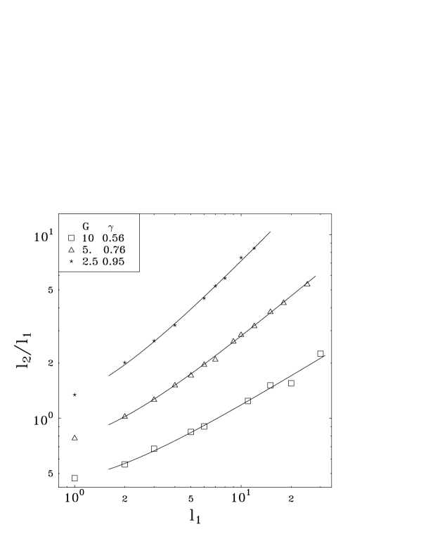
FIG. 2.: The factor of enhancement for the coherent propagation $l_{2}/l_{1}$ as a function of $l_{1}$ for few values of $G$. Both axes given in logarithmic scale. The $\gamma$ is the slope of the curve at the asymptotics $l_{1}\rightarrow\infty$ (81).

As one can see from the fig. 2 the deviations from linear behavior in the logarithm–logarithm plot for the $l_{2}/l_{1}$ turn out to be sufficiently weaker than for the participation ratio $P$. The solid curves on the figure corresponds to the least squares fitting with the formula

$$y=a+\gamma x+c\exp(-x)\ \ \ ,$$ (186)

$$y=\ln(l_{2}/l_{1})\ \ ,\ \ x=\ln(l_{1})\ \ .$$ (187)

This approximation corresponds to

$$l_{2}/l_{1}\sim l_{1}^{\displaystyle\gamma}\left(1+\frac{c}{l_{1}}\right)\ \ .$$ (188)

Thus, we have conjectured that the preassymptotic corrections decrease like $l_{1}^{-1}$. The values of the exponent $\gamma$ for different magnitude of the diagonal $G$ are

$$G=10.\ \ \ \ \gamma=0.56\,\pm 0.04\ \ ,$$ (189)

$$G=5.\,\ \ \ \ \ \gamma=0.76\,\pm 0.04\ \ ,$$ (190)

$$G=2.5\ \ \ \ \gamma=0.95\,\pm 0.04\ \ ,$$ (191)

In fact these three $\gamma$ may be considered as a main result of our paper. The pure statistical errors for this $\gamma$-s are of the order of a few percent and may be further improved easily. The main physical problem however is the proper choice of the fitting function (186). For example the data presented in the fig. 2 still allows one to use $y=a+\gamma x+cx^{2}$ instead of (186).

First of all, from the result (189) one may conclude with sure that the exponent $\gamma$ depends on the strength of the diagonal $G$. However, with only three points in hand we were afraid to fit the dependence $\gamma(G)$ by some smooth function. The physical conditions, evidently consistent with the data (189), for the function $\gamma(G)$ are $\gamma(G=\infty)=0$ and $\gamma(G=0)=const\sim 1$. Although the case $G\ll 1$ does not correspond to any mapping of the original TIP problem as we have said after the eq. (90). Also the connection between $G$, and $U$ and $t$ is described in eq. (90) and below.

The only rigorous way to confirm numerically the equation (188) and to exclude the more exotic dependence of $l_{2}$ on $l_{1}$ is to consider larger $l_{1}$. On the other hand, in using of the formula (185) we assume that the total size of the sample is large compared to the coherent propagation length $L\gg l_{2}$. Therefore below we would like to develop the method which in principle allows one to consider the coherent propagation with only the small matrices $L\sim l_{2}$ or even $L\ll l_{2}$ in hand.

Let us define the new function

$$F(L,l_{1})\equiv\langle\sqrt{1-R(L,l_{1})}\ \rangle=F(L/l_{2})\ \ \ .$$ (192)

Here the last equality will be our scaling hypothesis. Due to (183),(185) $F=1$ for the very small sample $L\ll l_{2}$ and $F\sim l_{2}/L$ for $L\gg l_{2}$. For $L\sim l_{2}$ the deviation of $F$ from trivial $F=1$ will measure the typical warp of the wave function on the circle. One should expect that this typical inhomogeneity of the wave function as well as the averaged shift of center of mass $\langle R(L,l_{1})\rangle$ will depend simply on the ratio of the size of the sample $L$ and the two-particle localization length $l_{2}$. Thus, it is natural to suppose that for $L\gg l_{1}$ the function $F(x)$ is universal in the sense that all dependence on $l_{1}$ in the r.h.s. of (192) is hidden in $l_{2}(l_{1})$. One still may have some doubts in this quite natural conjecture due to, e.g., the multifractal nature of the wave function. However, we may easily control its validity within our numerical calculations.

One may fix the value of $F$ and solve numerically the equation for $L$

$$F(L_{c},l_{1})=F(x_{c})=F_{c}\ \ \ ,$$ (193)

$$L_{c}=x_{c}(F_{c})\times l_{2}(l_{1})\ \ \ .$$ (194)

Here only the overall normalization factor $x_{c}$ depends on the value of $F_{c}$. Of course, the scaling behavior (192),(193) should be violated at $L\sim l_{1}$. However, because we have seen from fig. 2 that for large single particle localization length $l_{2}\gg l_{1}$ one may hope that (193) will be still valid even for $l_{1}\ll L\ll l_{2}$. Physically, this means that we are trying to find the manifestations of the finite coherent propagation length $l_{2}$ in the sample much smaller than this length.

FIG. 3.: The $\ln(L_{c})$ as a function of $\ln(l_{1})$ (84),(85) for $G=5$ and various values of $F_{c}=0.2,0.3,0.4,0.5,0.6,0.7,0.8$ (from the left to the right).

The dependence of the $\ln(L_{c})$ on the $\ln(l_{1})$ for $G=5.$ and for different values $F_{c}=0.2,0.3,0.4,0.5,0.6,0.7,0.8$ is presented in the fig. 3. At least six of this seven curves looks quite parallel which may be considered as the confirmation of the scaling hypothesis (192). Also it is natural that the corrections to scaling as it may be seen from the figure are stronger for larger values of $F_{c}$. In order to take into account at least the corrections to scaling proportional to $\sim 1/l_{1}$ we like in (186) have fitted our results by

$$y_{i}=a_{i}+(1+\gamma)x+c_{i}\exp(-x)\ \ \ ,$$ (195)

$$y_{i}=\ln(L_{c}(F_{c}))\ \ ,\ \ x=\ln(l_{1})\ \ ,$$ (196)

where $a_{i}$ and $c_{i}$ differs for different $F_{c}$ but $\gamma$ is the same for all seven curves of fig. 3. Finally the joint fitting (195) gives

$$\gamma=0.83\ \pm 0.04\ \ \ {\rm for}\ \ \ \ G=5.\ \ ,$$ (197)

in agreement with (189). The main advantage of this (192)-(195) indirect method of determination of $\gamma$ is that we have reached the value $l_{1}=90$ ($l_{2}\approx 1300$) by considering the $L\times L$ matrices with $L<1500$. For the direct method (185)-(188) for $G=5.$ in order to reach even $l_{1}=25$ we have to invoke the much larger matrices with $L\sim 2500$.

Of course, due to the logarithmic scale the progress made by going from fig. 2 to fig. 3 may look not so impressive and the result (197) due to the scaling hypothesis (192) may be considered as model dependent. Nevertheless we conclude from (197) that we see no evidence for the violation of the simple power law behavior (188) for $l_{2}$.

VII Conclusions

In the present paper we have tried to revise the issue of the enhancement of coherent propagation of two interacting particles in random potential predicted by D.L. Shepelyansky [1].

First of all, we definitely see the enhancement but it is of the different nature and has the different functional dependence from those usually considered. The existence of the enhancement itself is proved by considering the analytical estimate of the matrix element of interaction potential (27),(81),(84). Effectively the particle-particle interaction turns out to be enhanced in logarithm of the Anderson localization length times $\ln(l_{1})$. Moreover, after summation of high order contributions in this effective interaction this logarithm is most likely exponentiated so that $l_{2}/l_{1}\sim\exp\{\gamma\ln(l_{1})\}$ , where $\gamma=\gamma(U/t)$ .

Unfortunately the functional dependence of the two particle localization length (188) was found only numerically. Therefore we still can not completely exclude some other, rather exotic, dependence of $l_{2}$ on $l_{1}$. The equation (188) finds also some support in the very similar behavior of the inverse participation ratio $l_{ipr}$ (154) which was found analytically for the simplified model with the short sample.

The results (188),(154) were obtained by mapping of the original two-particle problem onto some random matrix model (87),(88),(188),(166). This means that we are able to explain only qualitatively the behavior of $l_{2}$. Therefore it is quite desirable if somebody will found the same behavior of the coherent propagation length as in our equation (188) in the direct calculation with the Hamiltonian (4) (some numerical results supporting (188) may be found in [3]). To this end the numerical method of ref. [5] seems to be very useful. The method of investigation of the effect of localization in the samples not large compared to the localization length described at the end of Section 6 being combined with the numerical method of [5] may also allow one to consider the larger range of variation of the coherent propagation length.

In general, may be the most interesting result of our paper is that we have found the nontrivial structure (or hierarchy of the elements) of the matrix of interaction (27),(81),(84) in the basis of noninteracting states (19),(43),(54). Just due to this hierarchy the matrix models we have to consider differ so drastically from those investigated before.

In this paper we consider only the interacting particles moving in exactly $1d$-random potential. It will be very interesting to generalize our approach for interacting particles in weak two and three dimensional random potential, which are currently the subject of intensive investigation [25].

Acknowledgments. Authors are thankful to V. F. Dmitriev, Y. Imry, I. V. Kolokolov, A. D. Mirlin, D. V. Savin, V. V. Sokolov, V. B. Telitsin, V. G. Zelevinsky and especially to O. P. Sushkov and D. L. Shepelyansky for numerous helpful discussions.

REFERENCES

- [1] D.L. Shepelyansky, Phys. Rev. Lett. 73, 2607 (1994).
- [2] Y. Imry, Europhys. Lett 30, 405 (1995).
- [3] K. Frahm, A. Müller-Groeling, J.-L. Pichard and D. Weinmann, Europhys. Lett. 31, 405 (1995).
- [4] D. Weinmann, A. Müller-Groeling, J.-L. Pichard and K. Frahm, Phys. Rev. Lett. 75, 1598 (1995).
-
[5]
F. von Oppen, T. Wettig and J. Müller,
Phys. Rev. Lett. 76, 491 (1996)
The actual enhancement parameter observed in this paper is rather weak . However, within the definition of used by authors the limit of switched of interaction corresponds to . Therefore effectively the observed enhancement is twice larger. - [6] P. Jacquod and D. L. Shepelyansky, Phys. Rev. Lett. 75, 3501 (1995).
- [7] Y. V. Fyodorov and A. D. Mirlin, Phys. Rev. B 52, R11580 (1995).
- [8] K. Frahm and A. Müller-Groeling, Europhys. Lett. 32, 385 (1995).
- [9] K. Frahm, A. Müller-Groeling, and J.-L. Pichard, Phys. Rev. Lett. 76, 1509 (1996).
- [10] D. Weinmann and J.-L. Pichard, Phys. Rev. Lett. 77, 1556 (1996).
- [11] F. Borgonovi and D. L. Shepelyansky, Journal de Physique I. 6(2) (1996) 287.
- [12] P. Jacquod, D. L. Shepelyansky and O. P. Sushkov, cond-mat/9605141. See however, the discussion at the end of our Section 2.
-
[13]
The propagation of interacting
particles in the random potential was considered also in:
O. N. Dorokhov, Sov. Phys.-JETP 71(2) (1990) 360.
However, the confining particle–particle interaction considered by Dorokhov seems to be very different from the short range interaction of ref. [1]. - [14] In the presence of, e.g., attractive interparticle interaction there evidently appear a few trivial molecular bound states. The size of this molecules is and the “molecular” localization length . More concretely, the size of the molecule for weak interaction (if the size of the molecule is larger than the lattice spacing) is (5,7). However, for very small one should also take into account the decay of the molecules due to interaction with the random potential. Anyway the number of molecular states is – much less than the number of coherent states.
- [15] One of the natural ways to investigate the effect of interaction is to consider the rigidity of spectrum for TIP as it was done in [10]. In accordance with our consideration of the large limit the authors of ref. [10] have observed the decrease of level repulsion for the strong interaction case as well as for the weak interaction one . We are thankful to J.-L. Pichard for discussion of this result.
- [16] I. M. Lifshits, S. A. Gredeskul, L. A. Pastur, Introduction to the theory of disordered systems. John Wiley and Sons, Inc., 1988.
- [17] L. Levitov, Europhys. Lett. 9, 83 (1989); Phys. Rev. Lett. 64, 547 (1990).
- [18] A. D. Mirlin, Y. V. Fyodorov, F. Dittes, J. Quezada, and T. H. Seligman, Phys. Rev. E, 54, 3221 (1996)
- [19] The authors of ref. [5] have fitted their results for any strength of the interaction by (3) with only one fixed value . This fixed value of is the most important difference of the result of [5] from our prediction. Because the large were not considered in [5] we would expect the most clear deviation from in their data for . In the notations of [5] the small are hidden in the small argument part of their fig. 1. However, just the small argument part of this figure demonstrates the largest deviation from the straight line expected by the authors. On the other hand, the center of the zone used for numerical investigation in [5] turns out to be just the most difficult case for the theoretical analysis. For example, the weak coupling limit does not work at all here because in the center of the zone energy conservation automatically leads to the momentum conservation ( in (81) see also discussion after the eq. (84)).
- [20] D. C. Thouless, Phys. Rev. Lett. 39, 1167 (1977).
- [21] See e.g. B. Kramer and A. MacKinnon, Rep. Prog. Phys. 56, 1469 (1993).
- [22] Y. V. Fyodorov, A. D. Mirlin, Int. J. Mod. Phys. B8, 3795 (1994).
- [23] To be more rigorous at this point one should introduce some . If the relative change of the participation ratio for the -th level at the -th step is less than , this correction is ignored. The “important” events are those with .
- [24] D. L. Shepelyansky, cond-mat/9603086.
-
[25]
Ya. M. Blanter, cond-mat/9604101;
B. L. Altshuler, Y. Gefen, A. Kamenev, and L. S. Levitov, cond-mat/9609132.