[

Analytical Long-Range Embedded-Atom Potentials

We present a systematical method for obtaining analytical long-range embedded-atom potentials based on the lattice-inversion method. The potentials converge faster (exponentially) than Sutton and Chen’s power-law potentials (Philos. Mag. Lett. 61, 2480(1990)). An interesting relationship between the embedded-atom method and the universal binding energy equation of Rose et al. (Phys. Rev. B 29, 2963 (1984)) is also pointed out. The potentials are tested by calculating the elastic constants, phonon dispersions, phase stabilities, surface properties and melting temperatures of the fcc transition metals. The results are overall in agreement with experimental or available ab initio data.

PACS:34.20.Cf, 61.50.L, 62.20.Dc

]

I Introduction

There are quite a few problems in atomistic simulation for which long-range potentials are needed. An important one is the problem of structural energy difference (SED). Normally the minimum SED is of the magnitude of one percent of the cohesive energy or so. Evidently if the potential range is only up to the second nearest neighbors, then a pair functional model will predict no energy difference between the fcc and hcp structures. We have to extend the ranges of potentials to further distance. Usually people impose a cut-off on the potentials and adjust the model parameters so that correct SED can be produced. However, the unphysical cut-off procedure thus becomes the dominant factor for predicting the SED: Suppose we fix the model parameters and change the cut-off distance, then it is highly possible to find that the SED varies in sign with respect to the cut-off distance(see Fig.1 in Ref. 1). The safe way to remove this drawback is to extend the range of the potentials so that the contributions from the furthest atoms become less than one percent of the cohesive energy. Fig. 1 illustrates that to get reliable SED between fcc and bcc for copper the potential range should be extended into the big circle (corresponding to some tolerable error bound). Only to that region (and beyond) does the universal binding energy relation (UBER) of Rose et al.  [2] decrease to the magnitude of the SED between fcc and bcc lattices. For alloys the problem will be more complex. There are some superstructures with very large unit cells. To calculate the heats of formation for these competing structures needs very long-range potentials. For calculating the elastic constants, the potential range is also important. For example, the predicted shear modulus $C^{\prime}$ of bcc structure is zero if a nearest-neighbor potential is used, so a potential range beyond nearest-neighbor distance is required for bcc structure. Long-range potentials are also needed for phonon calculation. In the case that the unit cell is very large, the potential range should be long enough so that all the atoms in the unit cell can interact with each other hence the force constants linking them do not vanish.

FIG. 1.: Schematical illustration for the need of long-range potential. The filled cirlces denote the radial distribution of the atom shells of fcc copper. The curve is the UBER for copper. The big circle shows the region to which the potential range should be extended.

To determine interatomic potentials, one has to assume some functional forms for them (such as exponential and power-law functions), and the potential parameters are fitted from experimental properties. The parameters can be exactly solved within Johnson’s nearest-neighbor model with exponential potentials [3] and Sutton and Chen’s long-range model with inverse power-law potentials [4]. Of course, Johnson’s model is not applicable in many cases because it is too short-range. On the other hand, as inverse power-laws, Sutton and Chen’s potentials converge, however, slower than the exponentials (this will be explained later). In molecular dynamics simulation, slow convergence of the potentials will result in the increasing of the time needed to make the neighbor list. In a long-range model that does not employ power-law functions, the conventional way to obtain the parameters is the numerical method of least-square fitting. The disadvantage of the numerical fitting method is that it is a little arbitary. Different authors may obtain different parameters, or the same author may obtain different parameters at different time, while a small variation of the parameters may lead to change of the long-range tail remarkable for the SED. This makes the conventional fitting method problematical when the fitted potentials are to be used to calculate something like phase stability and stacking fault energy. These properties are quite sensitive to the long-range tail which is, however, not very refined in the conventional fitting method.

In this paper, we present a systematical method of obtaining analytical long-range potentials with satisfactory convergence based on the lattice-inversion method (LIM). The LIM was first used by Carlsson, Gelatt and Ehrenreich (CGE) to get parameter-free pairwise potential from ab initio total energy calculation. [5] Recently, the inversion formula of CGE was recasted into a concise formulism by Chen based on the Möbius inversion transform in number theory  [6, 7, 8]. Nevertheless, the original two-body inversion scheme has, of course, some problems because of the lack of many-body contribution. Therefore, some many-body inversion schemes based on the $N$-body potential [9] and angularly-dependent Stillinger-Weber potential [10] were developed by Xie and Chen [11] and Bazant and Kaxiras  [12], respectively.

This paper is organized as follows. In Section II, we briefly introduce the LIM. In Section III, we present the lattice-inversion model for the embedded-atom method (EAM) [13]. In Section IV, we discuss the parametrization procedure in detail. In Section V, we present some calculated results. The paper is concluded in Section VI.

II The lattice-inversion method

The LIM can be traced to an early work by CGE. [5] The idea is to invert a function from its lattice sum which is sometimes easier to be obtained. For example, in the pair potential model (PPM), the cohesive energy can be written as the summation of the pair potential over the crystal lattice

$$E(R_{1})=(1/2)\sum_{m=1}^{\infty}w_{m}V(p_{m}R_{1})$$ (1)

where $w_{m}$ is the number of atoms on the $m$-th shell, $p_{m}$ is the ratio of the radius of the $m$-th shell to the nearest-neighbor distance. The cohesive energy as a function of lattice spacing can be calculated by using first-principles method, or simply taken as the UBER. Then as CGE suggested, one can use the following inversion formula to obtain the so-called ab initio pair potential $V(r)$

$\displaystyle V(r)=\frac{2}{w_{1}}E\left(\frac{r}{p_{1}}\right)-\sum_{m=2}^{\infty}\frac{2}{w_{1}}\frac{w_{m}}{2}\frac{2}{w_{1}}E\left(\frac{p_{m}r}{p_{1}^{2}}\right)$

$$+\sum_{m,n=2}^{\infty}\frac{2}{w_{1}}\frac{w_{m}}{2}\frac{2}{w_{1}}\frac{w_{n}}{w_{1}}\frac{2}{w_{1}}E\left(\frac{p_{m}p_{n}r}{p_{1}^{3}}\right)-\cdots$$ (2)

The multiple summations make the ordering for the inversion coefficients not obvious. It was not until recently that Chen put forward his elegant Möbius inversion formula on three-dimensional crystals. [8] The Chen-Möbius inversion formula is very simple

$$V(r)=2\sum_{m=1}^{\infty}\mu_{m}E(p_{m}r)$$ (3)

The Möbius coefficients $\mu_{m}$ can be determined by

$$\mu_{1} = {1}/{w_{1}}$$ (4)

$$\mu_{m} = -({1}/{w_{1}})\sum_{p_{k}|p_{m},k\neq m}\mu_{k}w_{l}\hskip 5.69046pt(m\geq 2)$$ (5)

where $l$ is the natural number which satisfies $p_{l}=p_{m}/p_{k}$. Obviously, Chen’s formula requires the set ${\bf P}=\{p_{m}|m\in{\bf N}\}$ should be a multiplication-close one, i.e., given two arbitrary elements $p_{i}$,$p_{j}$ $\in$ P, their product $p_{i}p_{j}$ should be in P too. Actually the crystal lattices sc, bcc, fcc, hcp and diamond etc. do not automatically satisfy this requirement. Therefore, before applying the Chen-Möbius formula we have to at first construct a close set ${\bf Q}$, which should include at least part of the elements in the orginal set ${\bf P}$. This task is easily done for sc and fcc: For them the set ${\bf P}$ is simply $\{\sqrt{i^{2}+j^{2}+k^{2}}R_{1}|i,j,k\in{\bf Z},i^{2}+j^{2}+k^{2}\neq 0\}$, we can construct a new set ${\bf Q}$=$\{\sqrt{n}R_{1}|n\in{\bf N}\}$, which covers ${\bf P}$. The numbers of atoms on the shell $\sqrt{n}R_{1}$ vanish if $n$ cannot be written as the square sum of three natural numbers $i^{2}+j^{2}+k^{2}$. But for other lattices such as bcc, it is difficult to find a natural close set which covers all the elements in the set ${\bf P}$= $\{\sqrt{i^{2}+j^{2}+k^{2}}a|i,j,k\in{\bf Z},i^{2}+j^{2}+k^{2}\neq 0\}\cup\sqrt{(i+1/2)^{2}+(j+1/2)^{2}+(k+1/2)^{2}}a|i,j,k\in{\bf Z}\}$, where $a$ is the lattice constant. However, for the present physical problem we do not have to construct a close set covering all the elements. Note that the expansion of eq.(1) should be convergent. That is to say, usually we can truncate at some shell, say, the $M$-th shell, beyond which the function $V(r)$ has become small enough to be neglected. So we can approximate eq.(1) by $E(R_{1})=\sum_{m=1}^{M}w_{m}V(p_{m}R_{1})$, then we have a set with $M$ elements ${\bf P}$= $\{p_{1},p_{2},\cdots,p_{M}\}$. We can easily generate a close set ${\bf Q}$ which covers ${\bf P}$: ${\bf Q}$= $\{p_{1}^{k_{1}}p_{2}^{k_{2}}\cdots p_{M}^{k_{M}}|k_{1},k_{2},\cdots,k_{M}=0,1,2,3,\cdots,k_{1}+k_{2}+\cdots+k_{M}\neq 0\}$. Re-ordering this close set from the smallest element to the biggest one, we get the set as ${\bf Q}$= $\{p_{m}^{{}^{\prime}}|p_{m}^{{}^{\prime}}<p_{m+1}^{{}^{\prime}},m\in{\bf N}\}$. Then we can rewrite eq.(1) as $E(R_{1})=(1/2)\sum_{n=1}^{\infty}w_{n}^{{}^{\prime}}V(p_{n}^{{}^{\prime}}R_{1})$, where $w_{n}^{{}^{\prime}}=w_{m}$ when $p_{n}^{{}^{\prime}}=p_{m}$ and vanishes when $p_{n}^{{}^{\prime}}$ equals none of the elements in P. The inversion is simply the same as eq.(3), with the Möbius coefficients $\mu_{n}^{{}^{\prime}}$ determined from $w_{n}^{{}^{\prime}}$.

In the one-dimensional case, eq.(3) becomes the number-theoretic Möbius inversion formula

$$V(r)=\sum_{n=1}^{\infty}\mu(n)E(nr)$$ (6)

where $\mu(n)$ is the number-theoretic Möbius function. This physical mapping (Fig.2) was first dicovered by Chen [6].

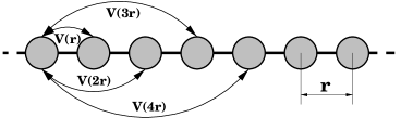
FIG. 2.: A physical mapping of the Möbius inversion theorem in arithmetic number theory.

Very recently, Bazant and Kaxiras have presented a novel scheme to obtain effective angularly-dependent many-body potentials for covalent materials by inversion of cohesive energy curves from many configurations [12]. Their method, together with our previous work for the EAM [11], have shown the potentiality of the LIM as a shortcut to obtain the effective interatomic potentials.

III The lattice-inversion embedded-atom model

Generally the physical properties we use to fit the potential parameters are related more closely to the lattice sums than to the individual potential function themsleves. Given the lattice sums of the pair potential $V(r)$ and electron density $f(r)$

$$\sum_{i}f(R_{i}) = \rho(R_{1})$$ (7)

$$(1/2)\sum_{i}V(R_{i}) = \Phi(R_{1})$$ (8)

We can easily rewrite the formulas of the bulk modulus and Voigt shear modulus

$$B=\frac{1}{18\Omega}\{\sum_{i}R_{i}^{2}[V_{\rm eff}^{{}^{\prime\prime}}(R_{i}) -\frac{1}{R_{i}}V^{{}^{\prime}}_{\rm eff}(R_{i})]$$ (10)

$$+2F^{{}^{\prime\prime}}(\rho_{e})[\sum_{i}R_{i}f^{{}^{\prime}}(R_{i})]^{2}\}$$

$$G=\frac{1}{30\Omega}\sum_{i}R_{i}^{2}[V_{\rm eff}^{{}^{\prime\prime}}(R_{i}) -\frac{1}{R_{i}}V^{{}^{\prime}}_{\rm eff}(R_{i})]$$ (11)

as

$$B =\frac{1}{9\Omega}\{R_{1}^{2}[\Phi^{{}^{\prime\prime}}(R_{1})+F^{{}^{\prime}}(\rho)\rho^{{}^{\prime\prime}}(R_{1})]$$ (13)

$$-R_{1}[\Phi^{{}^{\prime}}(R_{1})+F^{{}^{\prime}}(\rho)\rho^{{}^{\prime}}(R_{1})]+F^{{}^{\prime\prime}}(\rho)R_{1}^{2}[\rho^{{}^{\prime}}(R_{1})]^{2}\}$$

$$G =\frac{1}{15\Omega}\{R_{1}^{2}[\Phi^{{}^{\prime\prime}}(R_{1})+F^{{}^{\prime}}(\rho)\rho^{{}^{\prime\prime}}(R_{1})]$$ (15)

$$-R_{1}[\Phi^{{}^{\prime}}(R_{1})+F^{{}^{\prime}}(\rho)\rho^{{}^{\prime}}(R_{1})]\}$$

where $\Omega$ is the atomic volume, $V_{\rm eff}(r)$ is the effective pair potential $V_{\rm eff}(r)=V(r)+2F^{{}^{\prime}}(\rho)f(r)$. And for transforming eqs.(10) and (11) to the effective nearest neighbor forms of eqs.(13) and (15), the following relationship has been used: if there is a function $h(r)$ whose lattice sum is another function $H(R_{1})$, then

$$\sum_{i}R_{i}^{n}h^{(n)}(R_{i})=R_{1}^{n}H^{(n)}(R_{1})$$ (16)

Thus we have an equation related to the Cauchy pressure

$$9B\Omega-15G\Omega=F^{{}^{\prime\prime}}(\rho)R_{1}^{2}[\rho^{{}^{\prime}}(R_{1})]^{2}$$ (17)

On the other hand, the vacancy-formation energy

$$E_{v}=-\Phi+\sum_{i}[F(\rho-f(R_{i}))-F(\rho)]+E_{\rm relax}$$ (18)

can be approximately written as the lattice sum of the effective pair potential $E_{v}=(1/2)\sum_{i}V_{\rm eff}(R_{i})$, since the numbers of atoms on the shells are much greater than 1, and the negative relaxation energy further reduces the error. This approximation has been checked by a simple relaxation calculation in which only the nearest neighbor atoms around the vacancy site are allowed to relax. It is found that in the case of copper the calculated unrelaxed vacancy-formation energy is 1.34 eV, while the relaxed result is 1.31 eV, closer to the experimental value. Hence, the difference between the vacancy-formation energy and the sublimation energy can be written as

$$E_{s}-E_{v}=F^{{}^{\prime}}(\rho)\rho(R_{1})-F[\rho(R_{1})]$$ (19)

We can see from eqs.(17) and (19) that the nonlinearity of the embedding function reflects the many-body nature of the embedded-atom potential. If $F(\rho)$ is a linear function with respect to $\rho$ (corresponding to a PPM), then we have $3B=5G$ (the Cauchy relation) and $E_{s}=E_{v}$, which are the two well-known drawbacks of the PPM.

The nearest-neighbor distance of the equilibrium lattice can be obtained by minimizing the total binding energy

$$\Phi^{{}^{\prime}}(R_{1e})+F^{{}^{\prime}}(\rho_{e})\rho^{{}^{\prime}}(R_{1e})=0$$ (20)

Another condition we need to consider is the normalisation for the electron density. Integrating both sides of eq.(8) with respect to $R_{1}$

$$\sum_{m}\frac{w_{m}}{p_{m}^{3}}\int_{0}^{\infty}f(p_{m}R_{1})4\pi (p_{m}R_{1})^{2}d(p_{m}R_{1})$$ (22)

$$=\int_{0}^{\infty}4\pi R_{1}^{2}\rho(R_{1})dR_{1}$$

Note that the electron density $f(r)$ should be normalized $\int_{0}^{\infty}4\pi r^{2}f(r)dr=N$ (where $N$ is the number of electrons), we obtain

$$\int_{0}^{\infty}4\pi R_{1}^{2}\rho(R_{1})dR_{1}=S(3)N$$ (23)

where $S(3)=\sum_{m}w_{m}/p_{m}^{3}$. In alloy case, the parameter $N$ should be determined by considering the charge transfer. This consideration is based on empirical Miedema’s equation which well decribes the heats formation of binary alloys. The attractive term in Miedema’s equation is re-interpreted by Pettifor as the contribution of the electronegativity difference, which is related to the charge transfer. [14]

The embedding function in the present model is assumed to be a power-law one

$$F(\rho)=-A\rho^{1/\lambda}$$ (24)

$\lambda=1$ corresponds to the PPM, while $\lambda=2$ corresponds to the $N$-body potential of Finnis and Sinclair. [9] In the following section we shall show that with appropriate functional forms for the electron density and pair potential, this embedding function will produce exactly the UBER, and the parameter $\lambda$ is insensitive to the functional forms of the electron density and pair potential.

The electron density and pair potential in the present model are structure-dependent as we can see from their inverted formulas

$$f(r) = \mu_{1}\rho(p_{1}r)+\mu_{2}\rho(p_{2}r)+\mu_{3}\rho(p_{3}r)+\cdots$$ (25)

$$V(r) = 2\mu_{1}\Phi(p_{1}r)+2\mu_{2}\Phi(p_{2}r)+2\mu_{3}\Phi(p_{3}r)+\cdots$$ (26)

The functions of $f(r)$ and $V(r)$ are the linear combinations of their lattice-summed functions $\rho(R)$ and $\Phi(R)$, while the structural dependence is included in the Möbius inversion coefficients $\mu_{m}$ and the radius ratio $p_{m}$. Different kinds of functions for $\rho(R)$ and $\Phi(R)$ will be used to control the potential convergence, as shown in the next section.

IV Parametrization

A $\rho(R)$ and $\Phi(R)$ are exponential functions

It has been found by Banerjea and Smith using the effective-medium theory that the off-site electron density exhibits a universal relationship with respect to lattice spacing: $\rho^{*}=\exp(-a^{*})$, which was used to explain the physical origin of the UBER within the framework of local density approximation [15]. Based on the results of Hartree-Fock calculations, Mei, Davenport and Fernando also pointed out that the lattice sum of the electron density as a function of lattice constant shows exponential behaviour. [16] Therefore, it is plausible to take $\rho(R)$ as an exponential

$$\rho(R_{1})=\rho_{e}\exp\left[-\alpha\left(\frac{R_{1}}{R_{1e}}-1\right)\right]$$ (27)

As a short comment, we would like to point out that when the authors of Ref.  [16] came to the above equation they just used a complex function as $f(r)$=$f_{e}\sum_{l=0}^{k}c_{l}(R_{1e}/r)^{l}$ to fit it. One can see in the present method we do not have to fit. The individual function is accurately given by eq.(25).

The repulsive energy is often assumed to have a relation with the bond energy (i.e. the embedding energy in this case) like $U_{\rm rep}(R)\propto[U_{\rm bond}(R)]^{\gamma}$, where $\gamma$ is 2 according to the so-called Wolfsberg-Helmholtz approximation.  [17] Therefore, we assume $\Phi(R)$ is also an exponential function

$$\Phi(R_{1})=\Phi_{e}\exp\left[-\beta\left(\frac{R_{1}}{R_{1e}}-1\right)\right]$$ (28)

In our method the parameters can be exactly solved as if the model were a nearest neighbor one. The solutions are

$$\lambda = \frac{5GE_{s}}{3BE_{v}}$$ (29)

$$\alpha = \sqrt{\frac{\lambda(9\Omega B-15\Omega G)}{E_{s}-E_{v}}}$$ (31)

$$\beta = \frac{E_{s}-E_{v}}{E_{s}-\lambda E_{v}}\alpha$$ (33)

$$\Phi_{e} = \frac{E_{s}-\lambda E_{v}}{\lambda-1}$$ (35)

$$\rho_{e} = \frac{NS(3)\alpha^{3}e^{-\alpha}}{8\pi R_{1e}^{3}}$$ (37)

$$A = \frac{\lambda}{\lambda-1}(E_{s}-E_{v})\rho_{e}^{-1/\lambda}$$ (39)

The binding energy equation is a Morse-like function

$$E_{\rm coh}(R_{1})=\Phi_{e} \exp\left[-\beta\left(\frac{R_{1}}{R_{1e}}-1\right)\right]$$ (41)

$$-A\rho_{e}^{1/\lambda}\exp\left[-\frac{\alpha}{\lambda}\left(\frac{R_{1}}{R_{1e}}-1\right)\right]$$

Different from other equations of state, eq.(41) includes the inputs of the Cauchy pressure and vacancy-formation energy.

B $\rho(R)$ and $\Phi(R)$ are gaussian functions

It has been shown that in the present method all the parameters are analytically determined by the input physical properties, which are only for the equilibrium lattice. The potential convergence depends on the functional forms we take for $\rho(R)$ and $\Phi(R)$. The gaussian function is an alternative choice

$$\rho(R_{1}) = \rho_{e}\exp\left[-\alpha\left[\left(\frac{R_{1}}{R_{1e}}\right)^{2}-1\right]\right]$$ (42)

$$\Phi(R_{1}) = \Phi_{e}\exp\left[-\beta\left[\left(\frac{R_{1}}{R_{1e}}\right)^{2}-1\right]\right]$$ (43)

The solutions are the same with the above subsection except

$$\alpha = \frac{1}{2}\sqrt{\frac{\lambda(9\Omega B-15\Omega G)}{E_{s}-E_{v}}}$$ (44)

$$\rho_{e} = \left(\frac{\alpha}{\pi R_{1e}^{2}}\right)^{3/2}NS(3)e^{-\alpha}$$ (46)

The binding energy equation is

$$E_{\rm coh}(R_{1})=\Phi_{e} \exp\left[-\beta\left[\left(\frac{R_{1}}{R_{1e}}\right)^{2}-1\right]\right]$$ (48)

$$-A\rho_{e}^{1/\lambda}\exp\left[-\frac{\alpha}{\lambda}\left[\left(\frac{R_{1}}{R_{1e}}\right)^{2}-1\right]\right]$$

C $\rho(R)$ and $\Phi(R)$ are modified exponential functions

The electron density may not be a simple exponential function. As we know it is always a combination of some Slater orbitals $r^{n}e^{-\kappa r}$. In order to reflect this, we suppose

$$\rho(R_{1})=\rho_{e}\left(\frac{R_{1}}{R_{1e}}\right)^{n}\exp\left[-\alpha\left(\frac{R_{1}}{R_{1e}}-1\right)\right]$$ (49)

The pair potential remains the same as eq.(28). The solutions of $\lambda$ are

$\displaystyle\lambda=\frac{1}{2}\left(1+\lambda_{0}+n\frac{E_{s}-E_{v}}{9B\Omega}\right)$

$$\pm\frac{1}{2}\left[\left(1+\lambda_{0}+n\frac{E_{s}-E_{v}}{9B\Omega}\right)^{2}-4\lambda_{0}\left(1+n\frac{E_{s}-E_{v}}{15G\Omega}\right)\right]^{1/2}$$ (50)

where $\lambda_{0}={5GE_{s}}/{3BE_{v}}$. In this case, we have two solutions. Each of them can exactly reproduce the physical inputs. This simple example then implies that there may exist several different attractors leading to different results when the conventional fitting procedure is used to search for an approximate solution. This problem may merit a thorough investigation, and will not be discussed in the present paper. Note that $(E_{s}-E_{v})/18B\Omega\ll 1$ and $(E_{s}-E_{v})/15G\Omega\ll 1$, if $n$ is taken to be 1, then the approximate solutions will be $\lambda^{+}=\lambda_{0}$ and $\lambda^{-}=1$. The latter solution is just the PPM which is then excluded. The solutions for the remaining parameters are

$$\alpha = n+\sqrt{\frac{\lambda(9\Omega B-15\Omega G)}{E_{s}-E_{v}}}$$ (51)

$$\beta = \frac{E_{s}-E_{v}}{E_{s}-\lambda E_{v}}(\alpha-n)$$ (53)

$$\rho_{e} = \frac{NS(3)\alpha^{n+3}e^{-\alpha}}{4\pi R_{1e}^{3}\Gamma(n+3)}$$ (55)

The expressions for the other two parameter $\Phi_{e}$ and $A$ are identical with those presented in the first subsection.

The binding energy equation is

$$E_{\rm coh}(R_{1}) = \Phi_{e}\exp\left[-\beta\left(\frac{R_{1}}{R_{1e}}-1\right)\right]$$ (56)

$$- A\rho_{e}^{1/\lambda}\left(\frac{R_{1}}{R_{1e}}\right)^{n/\lambda}\exp\left[-\frac{\alpha}{\lambda}\left(\frac{R_{1}}{R_{1e}}-1\right)\right]$$ (57)

When $\alpha/\lambda=\beta$ and $\lambda=n$, the above equation is just the UBER

$$E_{\rm coh}(R_{1})=\frac{\Phi_{e}}{1-\beta} \left[1+\beta\left(\frac{R_{1}}{R_{1e}}-1\right)\right]$$ (59)

$$\times\exp\left[-\beta\left(\frac{R_{1}}{R_{1e}}-1\right)\right]$$

From the above subsections, one can find two points to support the power-law embedding function. The first point is that this embedding function (given by $A\rho_{e}^{1/\lambda}$ and $\lambda$) is independent on the given funcional forms of the electron density and pair potential. This physically underpins the local nature of the embedding function. It is also true when the pair potential and electron density take the power-law forms. The second is that the given binding energy equation is very close (and even identical) to the UBER. This consistency is necessary for a good description for the thermal expansion (the anharmonity effect) [18]. In some sense, the method may represent an embedded-atom explanation for the UBER.

If $\rho(R_{1})$ and $\Phi(R_{1})$ take the form of power law the solutions for the parameters will remain unchanged except that $\rho_{e}$ cannot be determined since the power-law function cannot be normalized. However, an alternative parameter $\xi_{e}$= $A\rho_{e}^{1/\lambda}$ can be determined, as is the case of Sutton-Chen’s potential. The inverted functions, for example the pair potential, is given as $V(r)=\Phi_{e}/S(\beta)(r/R_{1e})^{-\beta}$. While in the case of exponential, $V(r)<(\Phi_{e}/12)e^{\beta}[\exp(r/R_{1e})]^{-\beta}$. Since $S(\beta)$ is only a little greater than 12 and the paramters $\Phi_{e},\beta$ are the same in the two cases, the above two functions cross approximately at the NN distance. Beyond the NN distance, the exponential potential is smaller and decreases much faster than the power law.

FIG. 3.: The inverted electron densities and pair potentials (inset) for the noble metals. The unit of $f(r)$ is Å^-3.

Fig. 3 shows the typical shapes of the inverted pair potential and electron density, respectively. One can see from the figure that the inverted electron densities and pair potentials decrease rapidly. In our calculation, the cut-off is placed at about 3$a_{e}$, where the pair potential and electron density have been negligible.

V Applications of the potentials

The physical inputs for the present model are listed in Tab. I. The elastic moduli of Al are from Simmons and Wang [19], those of Ni, Pd, Pt, Cu, Ag and Au are from Foiles, Baskes and Daws [20]; Lattice constants and cohesive energies are all from Kittel [21]; Vacancy-formation energies for fcc transition metals are from Foiles, Baskes and Daw [20], and that for Al is from Ballufi [22]. We do not list the number of electrons since $\rho_{e}$ can be incorparated with $A$ as a parameter it is not used in monoatomic calculations. It is only important in alloy calculations, in which it descibes the charge transfer effect.

TABLE I.: The model inputs $a_{\rm e}$,$E_{\rm s}$,$E_{\rm v}$, $B$,$G$. $a_{e}$ is in Å, $E_{s}$ and $E_{v}$ are in eV, $B$ and $G$ are in 10¹¹N/m².

Element	$a_{e}$	$E_{s}$	$E_{v}$	$B$	$G$
Ni	3.52	4.44	1.7	1.804	0.95
Pd	3.89	3.89	1.54	1.95	0.54
Pt	3.92	5.84	1.6	2.83	0.65
Cu	3.61	3.49	1.3	1.38	0.55
Ag	4.09	2.95	1.1	1.04	0.34
Au	4.08	3.81	0.9	1.67	0.52
Al	4.05	3.39	0.7	0.76	0.266

A Structural stabilities

Phase stability is the first test for the long-range potentials. For copper, the EAM result $E_{\rm fcc-bcc}$ (25.8meV) falls in the middle of the nonrelativistic and semirelativistic ab initio values (-17.7 meV and -48.8 meV) reported by Lu, Wei and Zunger [23]. The EAM result for $E_{\rm fcc-diamond}$ equals 1.07 eV, also close to their ab initio result (1.35 eV) for diamond-like copper with the correction of nonspherical charge-density inside the muffin-tin sphere. For all the studied elements, the present model predicts the fcc structure to be the ground state (see Tab. II). However, similiar to Sutton and Chen’s potentials [4], the EAM result for $E_{\rm fcc-hcp}$ is virtually zero, so we did not print the binding energy curve for hcp in Fig.4. This failure is believed to be due to the absence of the angularly-dependent or higher order moment contributions. It has been pointed out by Ducastelle and Cyrot-Lackmann that it is mainly the third and fourth moments that are responsible for the SEDs among bcc, fcc and hcp candidates. [24]

FIG. 4.: The predicted phase stability of copper using the present model.

TABLE II.: The predicted structural energy differences for the fcc metals. The energies are in eV. The numbers in the parentheses denote the function types used: 1=exponential; 2=gaussian; 3=modified exponential.

Element	$E_{\rm fcc}-E_{\rm sc}$	$E_{\rm fcc}-E_{\rm bcc}$	$E_{\rm fcc}-E_{\rm diamond}$
Ni(2)	-0.58	-5.31$\times 10^{-2}$	-1.36
Pd(1)	-0.53	-3.42$\times 10^{-2}$	-1.21
Pt(1)	-0.62	-4.67$\times 10^{-2}$	-1.39
Cu(1)	-0.44	-2.58$\times 10^{-2}$	-1.07
Ag(1)	-0.40	-2.28$\times 10^{-2}$	-0.94
Au(1)	-0.35	-2.29$\times 10^{-2}$	-0.83
Al(3)	-0.28	-2.11$\times 10^{-2}$	-0.66

B Elastic constants and phonon eigenfrequencies

The comparison of the calculated and experimental data for the elastic constants $C_{11}$, $C_{12}$, $C_{44}$, the anisotropy ratios $C/C^{\prime}$ ($C=C_{44}$, $C^{\prime}=(C_{11}-C_{12})/2$), and the phonon longitudinal and transverse frequencies $\gamma_{L}$, $\gamma_{T}$ at the boundary of the Brillouin zone are shown in Fig. 5. The elastic constants were calculated by exerting the corresponding strain matrices to the lattice. The vibrational eigenfrequencies are calculated by diagonalizing the EAM dynamical matrix [25]. The experimental data for the elastic constants of Ni, Pd, Pt, Cu, Ag and Au are from Foiles, Baskes and Daw [20], those for Al are from Simmons and Wang [19]. The experimental data for the phonon eigenfrequencies are from Ref. [26]. The calculated results are overall in agreement with the experimental data. Fig. 6 shows the predicted phonon dispersion curves for copper along the high symmetry directions are in excellent agreement with the experimental data.

FIG. 5.: Comparison of calculated and experimental results for the elastic constants, the longitudinal and transverse phonon eigenfrequencies at the Brillouin-zone boundary. (a) $C_{11}$; (b) $C_{12}$; (c) $C_{44}$; (d)$\gamma_{L}$; (e)$\gamma_{T}$.

FIG. 6.: Comparison of the theoretical phonon dispersion curves of Cu (solid lines) with the experimental data (filled circles) along the high symmetry directions.

It has to be pointed out that when the present model is applied to the bcc transition metals with low anisotropic ratios, the calculated elastic constants $C^{\prime}$ and $C_{44}$ severely disagree with the experimental data, despite of that the bulk modulus and the Voigt shear modulus can be reproduced. This may imply that for the bcc transition metals the directional bonding is significant.

C Surface properties

To calculate surface properties, we employ a simulation box with size $10\times 10\times 10$ and periodically reproduced in $x$,$y$ and half $z$ directions (rather than a slab). For (111) surface, a periodic boundary condition with rhombic geometry has been applied. Relaxation is not considered in the calculation.

The calculated results for the unrelax surface energies of low index surfaces (100), (110) and (111) are listed in Tab. III, in comparison with the relaxed results of Foiles et al. [20]. The calculated results for the adsorption energies $E_{\rm ad}$ at different sites (see Fig. 7) and the hopping diffusion barriers $U_{\rm diff}$ as well as the island formation energies on the (100) surface are given in Tab. IV. The result of $U_{\rm diff}$ for Ag is close to the ab initio results 0.52 eV (LDA) and 0.45 eV (GGA) reported by Yu and Scheffler[28]. The binding energies $E_{\rm bind}$ of adatom dimers are calculated to be negative, suggesting that adatoms tend to form islands. For trimers on the (100) surface, the calculated results disfavor the one dimensional configuration.

FIG. 7.: Top view of adatoms geometries at (100) surface. (a) The four-fold hollow site (FFHS); (b) The two-fold bridge site (TFBS); (c) One-dimensional (1D) trimer; (d) Two-dimensional (2D) trimer.

TABLE III.: The calculated surface energies of low index surfaces. The first row are the present results. The second row are the theoretical results of Foiles et al.. The experimental data (average-face values) as well as the theoretical results are all taken from Ref. 27. The units are erg/cm².

Surfaces	Ni	Pd	Pt	Cu	Ag	Au	Al
$\gamma_{100}$	1702	1318	1485	1411	782	891	614
	1580	1370	1650	1280	705	918	—–
$\gamma_{110}$	1856	1451	1650	1533	855	945	680
	1730	1490	1750	1400	770	980	—–
$\gamma_{111}$	1595	1181	1286	1320	714	768	550
	1450	1220	1440	1170	620	790	—–
exp.	2380	2000	2490	1790	1240	1500	—–

TABLE IV.: The calculated adatom adsorption and island formation properties on (100) surface. The units are eV.

Properties	Ni	Pd	Pt	Cu	Ag	Au	Al
$E_{\rm ad}$ to FFHS	-3.59	-3.02	-4.61	-2.77	-2.20	-3.14	-2.85
$E_{\rm ad}$ to TFBS	-2.52	-2.48	-4.10	-2.21	-1.76	-2.93	-2.49
$U_{\rm diff}$	1.07	0.54	0.51	0.56	0.44	0.21	0.36
$E_{\rm bind}$(dimer)	-0.42	-0.50	-0.71	-0.37	-0.35	-0.49	-0.29
$E_{\rm bind}$(1D trimer)	-0.82	-0.97	-1.35	-0.71	-0.67	-0.94	-0.55
$E_{\rm bind}$(2D trimer)	-0.90	-1.02	-1.39	-0.78	-0.72	-0.97	-0.58

D Molecular dynamics

In the above subsections the calculations are static. In this subsection, the potentials are tested in the constant-volume-temperature molecular dynamics (NVT-MD) simulation for melting processes for Cu and Pt. The simulation box contains 500 atoms. Gear predictor-corrector algorithm and Verlet neighbor list are applied. The time step is one femtosecond (10^-15 s). The ensemble average of the origin-independent translational order parameter is calculated after equilibration of at least 5000 steps

$$\sigma^{2}=\left\langle\left[\frac{1}{N}\sum_{i}\cos\left({\bf K}\cdot{\bf R}_{i}\right)\right]^{2}+\left[\frac{1}{N}\sum_{i}\sin\left({\bf K}\cdot{\bf R}_{i}\right)\right]^{2}\right\rangle$$ (60)

where $N$ is the number of atoms in the box, ${\bf K}$ is the reciprocal basis vector for the initial structure (for example, ${\bf K}=2\pi/a(-1,1,-1)$ for fcc lattice), and ${\bf R}_{i}$ are the position vectors for the atoms. Fig. 8 shows the order paramters as a function of temperature for Cu and Pt. In comparison with experimental data, the melting points are underestimated by an amount of 200-300 K. Our result of Cu is worse than that of Foiles and Adams [29] (1340 K), but that of Pt is better than theirs (1480 K). Fig.9 shows the pair distribution functions $g(r)$ of Cu at different temperatures.

FIG. 8.: Translational order parameters versus temperature for Cu and Pt. The experimental melting points for Cu(1358K) and Pt(2045K) are denoted by the two vertical solid lines.

FIG. 9.: Pair distribution functions of Cu at different temperatures.

We also simulated the melting of a slab. The size of the simulation box is 5$\times$5$\times$20, while that of the slab is 5$\times$5$\times$10 (containing 21 atomic layers or 1050 atoms). The slab is placed at the center of the simulation box, which is large enough to ensure that the slab does not interact with its images. The atomic configuration is described by the density profile $N(z)$ along the direction perpendicular to the slab. $N(z)$ is obtained by averaging over 1000 steps after running 20000 steps. Surface premelting is observed at 900 K, and the liquid fronts propagate inward when the temperature rises (920K). At 950K the slab completely melts.

FIG. 10.: Density profiles along the direction perpendicular to the slab of Cu at different temperatures.

The simulation results suggest that melting is a surface-initiated process. It would be interesting to investigate the temperature dependence of the depth of the melten layer. On the other hand, does the solidification process also begin from the surface, or from the core?

VI Concluding remarks

We have presented a systematical method of obtaining long-range embedded-atom potentials. The model parameters can be obtained explicitly from six physical inputs and the individual potentials are inverted from the analytical functions of lattice sums thus arbitary fitting can be avoided. It is shown that the model is able to produce satisfactory results of elastic constants, phonon eigenfrequencies, phase stabilities, surface properties and melting points for the fcc transition metals. The potentials are suitable for computer simulation because of their rapid convergence.

Deriving interatomic potentials from ab initio calculations when the experimental data are not available has become an abvious trend in the world of material simulation. [30] The reason has been explained very well in a recent paper by Payne et al. [31]. In this regard, the present method (as well as the method of Bazant and Kaxiras[12]) may represent an idea of bridging the gap between material theory and electronic structure theory by the method of inverting ab initio EAM potentials (or angularly dependent many-body potentials) from first-principles calculations. The ab initio binding energy curve can be decomposed into repulsive and attractive parts, representing the contributions of the pair potential and embedding energy respectively. By using our method, the ab initio EAM potentials can be obtained by inverting from the corresponding parts.

The present model is easy to be generalized to the alloy case by assuming that the pair potential between unlike atoms is given by Johnson’s formula $V_{ab}(r)=({1}/{2})\{[{f_{b}(r)}/{f_{a}(r)}]V_{aa}(r)+[{f_{a}(r)}/{f_{b}(r)}]V_{bb}(r)\}$.  [32] Finally it should be pointed out that the present model fails in predicting the bcc transition metals. Modifying the functional forms of $\rho$, $\Phi$ and $F(\rho)$ does not help much to solve this difficulty.

Acknowledgments: Q.X. gratefully thanks the Max-Planck-Institut für Physik komplexer Systeme for hospitality. This paper is dedicated to the 60th Birthday of Prof. N.X. Chen.

REFERENCES

- [1] F.Cleri and V.Rosato, Phys. Rev. B 48, 22 (1993)
- [2] J.H.Rose, J.R.Smith, F.Guinea and J. Ferrante, Phys. Rev. B 29, 2963 (1984)
- [3] R.A.Johnson, Phys. Rev. B 37, 3924 (1988)
- [4] A.P.Sutton and J.Chen, Philos. Mag. Lett. 61, 2480(1990)
- [5] A.E.Carlsson, C.D.Gelatt, and H.Ehrenreich, Philos. Mag. A 41, 241 (1980)
- [6] N.X.Chen, Phys. Rev. Lett. 64, 1193 (1990)
- [7] J.Maddox, Nature (London) 344, 377 (1990)
- [8] N.X.Chen, Z.D.Chen, and Y.C.Wei, Phys. Rev. E 55, R5 (1997)
- [9] M.W.Finnis and J.E.Sinclair, Philos. Mag. A 50, 45 (1984)
- [10] F.Stillinger and T. Weber, Phys. Rev. B 31, 5262 (1985)
- [11] Q. Xie and N.X.Chen, Phys. Rev. B 51, 15856 (1995)
- [12] M.Z.Bazant and E. Kaxiras, Phys. Rev. Lett. 77, 4370 (1996)
- [13] M.S.Daw and M.I.Baskes, Phys. Rev. Lett. 50, 1285 (1983); Phys. Rev. B 29, 6443 (1984)
- [14] D.G.Pettifor, in Physical Metallurgy, edited by R.W.Cahn and P.Haasen (Elsevier, Amsterdam, 1996) 4th edn., p. 111
- [15] A.Banerjea and J.R.Smith, Phys. Rev. B 37, 6632 (1988)
- [16] J.Mei, J.W.Davenport, and G.W.Fernado, Phys. Rev. B 43, 4653 (1991)
- [17] D.G.Pettifor, Bonding and Structure of Molecules and Solids (Oxford University Press, Oxford, 1995) p.65
- [18] S.M.Foiles and M.S.Daw, Phys. Rev. B 38, 12643 (1988)
- [19] G.Simmons and H.Wang, Single Crystal Elastic Constants and Calculated Aggregate Properties: A Handbook (MIT Press, Cambridge, 1971)
- [20] S.M.Foiles, M.I.Baskes, and M.S.Daw, Phys. Rev. B 33, 7983 (1986)
- [21] C.Kittel, Introduction to Solid State Physics, 6th edn. (Wiley, New York, 1986)
- [22] R.W.Ballufi, J. Nucl. Mater. 69&70, 240 (1978)
- [23] Z.W.Lu, S.H.Wei, and A.Zunger, Phys. Rev. B 41, 2699(1990)
- [24] F.Ducastelle and F.Cyrot-Lackmann, J. Phys. Chem. Solids 31, 1295 (1970)
- [25] M.S. Daw and R.D. Hatcher, Solid State Commun. 56, 697 (1985)
- [26] For Ni, R.J.Birgeneau et al., Phys. Rev. 136, 1359(1964); For Pd, A.P.Miller and B.N.Brockhouse, Can. J. Phys. bf 49, 704(1971); For Pt, D.H.Dutton and B.N.Brockhouse, Can. J. Phys. 50,2915(1972); For Cu, G.Nilsson and S.Rolandson, Phys. Rev. B 7, 2393(1973); For Ag, W.A.Kamitakahara and B.N.Brockhouse, Phys. Lett. 29A, 639(1969); For Au, J.W.Lynn, H.G.Smith, and R.M.Nicklow, Phys. Rev. B 8, 3493 (1973); For Al, G.Gilat and R.M.Nicklow, Phys. Rev. 143, 487(1966).
- [27] M.S.Daw, S.M.Foiles, and M.I.Baskes, Mater. Sci. Rep. 9, 251 (1993)
- [28] B.D. Yu and M. Scheffler, Phys. Rev. Lett. 77, 1095 (1996)
- [29] S.M.Foiles and J.B.Adams, Phys. Rev. B 40, 5909 (1989)
- [30] M. Yan et al., Phys. Rev. B 47, 5571 (1993)
- [31] M.C.Payne, I.J.Robertson, D.Thomson, and V.Heine, Philos. Mag. B 73, 191 (1996)
- [32] R.A.Johnson, Phys. Rev. B 39, 12554 (1989)