Replica Symmetry Breaking and the Kuhn-Tucker Cavity Method in simple and multilayer Perceptrons

Abstract

Within a Kuhn-Tucker cavity method introduced in a former paper, we study optimal stability learning for situations, where in the replica formalism the replica symmetry may be broken, namely

(i) the case of a simple perceptron above the critical loading, and

(ii) the case of two-layer AND-perceptrons, if one learns with maximal stability.

We find that the deviation of our cavity solution from the replica symmetric one in these cases is a clear indication of the necessity of replica symmetry breaking. In any case the cavity solution tends to underestimate the storage capabilities of the networks.

1 Introduction

In a recent paper, [1], we introduced a new kind of cavity method, with which we could solve the learning problem for perceptrons with $Q$- and $Q^{\prime}$ state Potts model input and output neurons. In this method, the Kuhn-Tucker conditions, which lead to optimal stability in AdaTron type learning processes, have been built into the cavity formulation. In subsequent papers we extended this method to the problem of the generalization ability of a perceptron trained for optimal stability [2], and to the problem of storing of correlated patterns [3].

In the present paper, we apply our method to cases where in the replica formalism the replica symmetry is broken, namely (i) to perceptrons with Ising neurons above the critical loading and (ii) to two-layer AND perceptrons.

Cavity ideas were first applied to neural networks by Mézard, [4], and Kinzel and Opper, [5]. The approach of Griniasty, [6], whose work will be discussed below in comparison with our own findings, employs ideas introduced by Mezard. Our formulation of the cavity method, on the other hand, was inspired by the just-mentioned work of Kinzel and Opper. In another original approach, Wong [7] employs ideas which are related to ours and Griniasty’s.

2 Simple perceptrons above the critical loading

We use the definitions as in [2], which are simpler than those we had to introduce for the Potts model case [1]. Our perceptron has $N$ input neurons $k=1,...,N$, whose possible states are $s_{k}=\pm 1$, and one output neuron $s^{\prime}$, also with possible states $\pm 1$. The couplings leading from the input neurons to the output neuron are assumed to be real numbers, which are collected into the coupling vector $\underline{J}:=(J_{1},...,J_{N})$ with the Euclidean length $L:=|\underline{J}|=(J_{1}^{2}+...+J_{N}^{2})^{1/2}$, which is kept fixed, while the components $J_{k}$ are adapted to certain tasks by ”training processes” (see below). The relation between input and output is

$$s^{\prime}=\hbox{sign}\left(\sum_{k=1}^{N}\,J_{k}\,s_{k}\,\right)\quad,$$ (1)

which can be considered as a binary classification of the possible inputs, or as answers on questions.

Now we assume that there is a training set of $p$ input-output pairs, where the inputs are $\underline{\xi}^{\mu}:=(\xi_{1}^{\mu},...,\xi_{N}^{\mu})$ for $\mu=1,...,p$, and the corresponding desired outputs are $\zeta^{\mu}$. Here and in the following, unless otherwise stated, we assume that all input components and the outputs are independent random numbers, which take the values $\pm 1$ with equal probability.

The optimization task, which the perceptron then has to fulfill in course of the training by adaptation of the components of the coupling vector $\underline{J}$, is the minimization of a Hamiltonian, which performs a weighted count of bad classifications (see below) of the training examples. Among these Hamiltonians are that of Gardner and Derrida, [8], which simply counts the bad classifications, namely

$${\cal H}:=\sum_{\mu}V(E^{\mu}):=\sum_{\mu}\theta(\kappa-(E^{\mu}/L))\,.$$ (2)

Here $\theta(x)=1$ for $x>0$, $=0$ else, and $E^{\mu}$ is defined as usual as the ”oriented field” acting on pattern $\mu$,

$$E^{\mu}=\zeta^{\mu}\sum_{k=1}^{N}J_{k}\xi_{k}^{\mu}\,,$$ (3)

while $L=|\underline{J}|$ as above. Bad classifications are those, where $E^{\mu}/L$ is $<\kappa$, i.e. for $\kappa>0$ they are not necessarily wrong but lack a prescribed amount of stability, which is measured by $\kappa$.

There are $p=:\alpha\cdot N$ such ”questions with prescribed answers”, i.e. $\mu=1,...,p$, and it is assumed that the loading parameter $\alpha$ remains finite, while $N\to\infty$ and $p\to\infty$. Furthermore, the stability parameter $\kappa$ is to be maximized, if error-free classification (i.e. ${\cal H}=0$) is possible.

Gardner and Derrida, [8], evaluated not only the number of errors $\cal H$ above the critical loading $\alpha_{c}(\kappa)$, where for positive $\kappa$ error-free classification is no longer possible, but they also tried to evaluate the so-called Almeida-Thouless-line $\alpha_{AT}(\kappa)$. Above this line, within the replica formalism, replica symmetry breaking (RSB) is necessary. Surprisingly, Gardner and Derrida found in [8] that $\alpha_{AT}>\alpha_{c}$ for $\kappa>0$: However, this was due to a subtle integration error recently discovered by Bouten, [9], who proved that $\alpha_{AT}(\kappa)=\alpha_{c}(\kappa)$, as expected. Bouten also showed that replica symmetry is always broken, if the distribution of local fields possesses a gap. So these results, on which we will comment later, provide a test for our cavity approach.

Other Hamiltonians, on which we comment at a later stage, are (see [10, 11]) the Perceptron function and the AdaTron function with

$$V(E^{\mu})=[\kappa-(E^{\mu}/L)]^{x}\cdot\theta[\kappa-(E^{\mu}/L)],$$ (4)

with $x=1$ and $x=2$, respectively.

2.1 Representation of optimal couplings

Instead of minimizing the weighted error rate $f(\alpha,\kappa):={\cal H}/p$, one can of course also maximize $\kappa(\alpha,f)$ for the given training set. Since we are above the critical loading $\alpha_{c}(\kappa)$, $f\cdot p$ of the training examples are badly classified. There is however an exponentially large number $\cal N$ of partitions of the training set into a ”good fraction” and a ”waste fraction” of size $(1-f)\cdot p$ and $f\cdot p$, respectively, from which one has to choose the optimal one. Namely, ${\cal N}\simeq\exp(c\cdot p)$, with $c=-f\,\ln f-(1-f)\,\ln(1-f)$. We nevertheless assume, that every one of these combinations has been trained for optimal stability, e.g. with the AdaTron algorithm [12]. The optimal perceptron with error rate $f$ is then given by the partition leading to maximal $\kappa$.

The couplings of a perceptron trained for optimal stability can always be expressed in the form [12]

$$J_{k}=\frac{1}{N}\sum_{\mu\in\{(1-f)p\}}x^{\mu}\zeta^{\mu}\xi_{k}^{\mu}$$ (5)

with the so-called “embedding strengths” $x^{\mu}$ of patterns, which do not belong to the $fp$ badly classified patterns. As can be shown using Lagrangian multipliers [12, 1], these embedding strengths have to fulfill the so called Kuhn-Tucker conditions, see below. Without restriction of generality, these are usually formulated by fixing the length $L$ of the coupling vector $\underline{J}$ in such a way that the stability limit for $\kappa>0$ corresponds to $E^{\mu}=1$, i.e. $L=\kappa^{-1}$. With this convention, which we always use in the following, unless otherwise stated, the Kuhn-Tucker conditions are :

$$\hbox{either}\quad(x^{\mu}>0\quad\hbox{and}\quad E^{\mu}=1)\quad\hbox{or}\quad(x^{\mu}=0\quad\hbox{and}\quad E^{\mu}>1)\>.$$ (6)

In fact, the AdaTron algorithm (without overrelaxation)

$$\delta x^{\mu}=\hbox{max}(-x^{\mu},1-E^{\mu})\qquad\hbox{(sequentially or in parallel)}$$ (7)

simply fixes the $x^{\mu}$ repeatedly to values which fulfill (6): If it converges, the conditions are necessarily obeyed.

Using the “oriented correlation” matrix

$$B^{\mu\nu}=\zeta^{\mu}\zeta^{\nu}\frac{1}{N}\sum_{k=1}^{N}\xi_{k}^{\mu}\xi_{k}^{\nu}\,.$$ (8)

and the definitions (3) and(5), we can write for the oriented field $E^{\mu}$

$$E^{\mu}=\sum_{\nu}B^{\mu\nu}x^{\nu}\;.$$ (9)

With the Kuhn-Tucker conditions we have finally

$$L^{2} = \sum_{\mu,\nu}x^{\mu}B^{\mu\nu}x^{\nu}=\frac{1}{N}\sum_{\mu}x^{\mu}\quad.$$ (10)

The basic idea of the cavity method here is, to add a pattern, i.e. the “cavity”, to a set of perfectly trained patterns. By calculating the necessary adjustments to embed this pattern we gain valuable information about the whole system. As in [1], we therefore add a new ”question with desired answer” $(\underline{\xi}^{0},\zeta^{0})$ to the training set, assuming one simple groundstate.

We note that the distribution of the oriented fields $\tilde{E}^{0}$ acting on it, before any further adaptation has been performed, which in the following always will be indicated by the  $\tilde{}$ , is Gaussian with average 0 and variance $|\underline{J}|^{2}=L^{2}=\kappa^{-2}$. Of course the error rate $f$ has to remain constant. Therefore, as will be seen below, the best strategy is, to give up and add the new pattern to the ”waste fraction of the training set”, if the oriented field $\tilde{E}^{0}$ acting on $\underline{\xi}^{0}$ is smaller than a certain number $Z<1$. For self-consistency, $Z$ is determined by

$$f=\int\limits_{-\infty}^{Z}{\hbox{d}}\tilde{E}^{0}\,{\frac{\exp[-(\tilde{E}^{0})^{2}/2L^{2}]}{\sqrt{2\pi L^{2}}}}=\int\limits_{-\infty}^{z}{\hbox{d}}t\frac{\exp(-t^{2}/2)}{\sqrt{2\pi}}\,,$$ (11)

where $t:=\tilde{E}^{0}/L$ and $z:=Z/L$. On the other hand, if $\tilde{E}^{0}$ is $>1$, then it is not necessary to embed $\underline{\xi}^{0}$ in the couplings, since it can be added to the set of those correctly classified training patterns, which need no explicit embedding (see [13]) by the Adatron algorithm, [12]. Thus, only for $Z<\tilde{E}^{0}\leq 1$, i.e. $z<t\leq\kappa$, the new pattern must be embedded in the couplings, and the implementation strength $x^{\mu}$ of the other patterns must be corrected by $\delta x^{\mu}$ (see below), to compensate for the influence of the new pattern.

As we have just seen, the parallel AdaTron algorithm would in a first step try to embed $\underline{\xi}^{0}$, if necessary, with the ”bare” embedding $x^{0}=1-\tilde{E}^{0}$. This generates a perturbation $B^{\mu 0}x^{0}$ of the pattern $\mu$. In a second parallel step, all those patterns $\mu$, which are stored explicitly, then have to respond by $\delta x^{\mu}=-B^{\mu 0}x^{0}$ to the disturbation by $x^{0}$, because the Kuhn-Tucker conditions still have to be fulfilled. At pattern 0 these corrections generate a response field

$$g\,x^{0}=\sum_{\mu,(x^{\mu}>0)}B^{0\mu}\delta x^{\mu}=-\sum_{\mu,(x^{\mu}>0)}(B^{0\mu})^{2}x^{0}\,\,,$$ (12)

which reduces the effect of the AdaTron step with $x^{0}$. Therefore, one has to enhance $x^{0}=1-\tilde{E}^{0}$ by an amplification factor 1/(1+g) ($>1$). Now the $(B^{0\mu})^{2}$ are $1/N$ on average, see (8). Therefore one gets immediately

$$\sum_{\mu,(x^{\mu}>0)}(B^{0\mu})^{2}=\alpha\cdot P(x^{\mu}>0)=:\alpha_{\hbox{\scriptsize eff}}\quad.$$ (13)

$\alpha_{\hbox{\scriptsize eff}}$ is the percentage of exhausted degrees of freedom, i.e., if pattern 0 is as typical as the other random patterns $\mu=1,\ldots,p$, one has to postulate

$$g=-\alpha_{\hbox{\scriptsize eff}}=-\alpha\cdot P(Z<\tilde{E}^{0}<1)=-\alpha\int_{z}^{\kappa}{\cal D}t\quad\stackrel{{\scriptstyle!}}{{\geq}}(-1)\quad.$$ (14)

Note that we have constructed our algorithm in such a way that the further correction steps, which are necessary to regain the Kuhn-Tucker conditions exactly, do not change the response at pattern 0 in the thermodynamic limit when convergence is achieved. A proof is given in the Appendix, where we also show that in this limit one can assume that the $x^{\mu}$ and $B^{\mu\nu}$ are statistically independent.

With our approach, the final embedding strength for $\underline{\xi}^{0}$ is then given by $(1-\tilde{E}^{0})/(1+g)$. Furthermore, we now identify the distribution of embedding strengths of all patterns with that of pattern $\underline{\xi}^{0}$. Putting the Gaussian distribution of the cavity field $\tilde{E}^{0}$, felt before training, into (10) gives

$$L^{2}=\alpha L\int_{z}^{\kappa}{\cal D}t\,\frac{\kappa-t}{1+g}\;.$$ (15)

With $L=\kappa^{-1}$ this implies

$$1=\frac{\alpha}{1+g}\int\limits_{z}^{\kappa}{\cal D}t\,(\kappa-t)\kappa\;.$$ (16)

After multiplication with $1+g$, this finally leads to our ”Kuhn-Tucker cavity result”

$$1 = \alpha\int\limits_{z}^{\kappa}{\cal D}t+\alpha\kappa\int\limits_{z}^{\kappa}{\cal D}t\,(\kappa-t)$$ (17)

$$= \alpha\,\,(1+\kappa^{2})\int\limits_{z}^{\kappa}{\cal D}t+\frac{\alpha\kappa}{\sqrt{2\pi}}(e^{-\kappa^{2}/2}-e^{-z^{2}/2})\,.$$ (18)

This result will now be compared with that of the cavity approaches of Griniasty, [6], and Wong [7]. Their different result is equivalent to the replica formalism in the replica-symmetric approximation, [8, 10]; therefore we use the suffix ”RS” to indicate their result. We have already shown in [1] that below $\alpha_{c}$, where replica-symmetry is exact, our Kuhn-Tucker cavity approach and the RS approach agree; however in the present situation, where $\alpha$ is $>\alpha_{c}$, they disagree.

When Griniasty derives the constant of integration in [6], he uses a simple method which in all cases known to us gives the correct RS result: The reaction factor $g$ is assumed to vanish, while at the same time also the $B^{\mu\nu}$ with $\mu\neq\nu$ are neglected. With these two neglections one obtains instead of eqn. (10)

$$L^{2} = \frac{1}{N}\,\vec{x}^{\,T}_{\hbox{\tiny RS}}\!\stackrel{{\scriptstyle\leftrightarrow}}{{B}}_{\hbox{\tiny RS}}\vec{x}_{\hbox{\tiny RS}}\>=\>\frac{1}{N}\sum_{\mu}(x^{\mu}_{\hbox{\tiny RS}})^{2}\quad.$$ (19)

Thus, instead of eqs. (17) and (18), the ”RS” cavity result would be

$$1 = \alpha_{\hbox{\tiny RS}}\int\limits_{z}^{\kappa}{\cal D}t\>(\kappa-t)^{2}$$ (20)

$$= \alpha_{\hbox{\tiny RS}}(1+\kappa^{2})\int\limits_{z}^{\kappa}{\cal D}t\>+\>\frac{\alpha_{\hbox{\tiny RS}}\kappa}{\sqrt{2\pi}}(e^{-\kappa^{2}/2}-e^{-z^{2}/2})+\underbrace{\frac{\alpha_{\hbox{\tiny RS}}}{\sqrt{2\pi}}(z-\kappa)e^{-z^{2}/2}}_{=:M}\quad.\qquad$$

Eqn. (20), which is identical with the result obtained by Griniasty [6] or Wong [7], agrees with the result of the replica calculation of Gardner and Derrida [8, 10] from the replica-symmetric approximation; the expression abbreviated by $M$ in eqn. (20) yields the difference between our $\alpha_{\hbox{\tiny Cav}}$ (=$\alpha$ obtained from eqn. (18)) and $\alpha_{\hbox{\tiny RS}}$. Because of $z<\kappa$, it is $M\leq 0$ and therefore $\alpha_{\hbox{\tiny RS}}\geq\alpha_{\hbox{\tiny Cav}}$. For $z\to-\infty$, i.e. for $f\to 0$, one has $M=0$, and thus for $\alpha\leq\alpha_{c}$ it is $\alpha_{\hbox{\tiny RS}}=\alpha_{\hbox{\tiny Cav}}$, as already mentioned.

Although the numerical results differ, there is an interesting formal relationship between the basic equations in Wong’s approach [7] and the one presented here: Eqn. (6) in [7] agrees formally with our eqn. (16), and our reaction strength $g$ corresponds to $-\alpha\cdot\chi$ in [7]. However $-\alpha\cdot\chi$ in [7] differs from our $g$, which is given by eqn. (14), by a term corresponding just to the expression $M$ in eqn. (20). The difference arises from a $\delta$-function contribution to $\lambda^{\prime}(t)$ at $t=z$ in [7], where $\lambda(t)$ and $t$ in [7] are the oriented fields after training and before training, respectively. Probably this difference, which only comes into play above $\alpha_{c}$, where $M$ is $\neq 0$, is relevant with respect to the combinatorial explosion, which conflicts with the assumption of a unique optimum made in all the approaches. Research on this problem is in progress.

In Fig. 1, for error rates of $f=0.2$ and 0.02, the learning capacities $\alpha(\kappa,f)=\alpha_{\hbox{\tiny Cav}}$ and $\alpha_{\hbox{\tiny RS}}$, respectively, as obtained from our Kuhn-Tucker cavity theory, eqn. (17), and with the replica-symmetric approximation (20) respectively, are plotted against the stability $\kappa$. Obviously, the learning capacity obtained with the Kuhn-Tucker cavity theory is lower, particularly at small values of $\kappa$, i.e. for $\kappa=0$ and $f=0.2$, $\alpha_{\hbox{\tiny Cav}}$ is only 10/3, whereas $\alpha_{\hbox{\tiny RS}}$ is 15.53. This means at the same time that for given $\kappa$ and $\alpha$, our error rate $f$ would be larger than that obtained with eqn. (20). This is a strong hint that the assumption of a unique optimum for the distribution of those patterns, which are put to waste, is wrong. Therefore, one cannot say in advance, which approach is better: Rather what has been gained is the following: Since both approaches agree below $\alpha_{c}(\kappa,f=0)$, but not for $f>0$, we can use the different results as a criterion for the necessity of replica-symmetry breaking for $f>0$, which agrees with the recent rigorous proof of [9].

2.2 Comparison with a One-Step-RSB calculation

Majer et al., [11], have performed a calculation above $\alpha_{c}(\kappa,f=0)$ within a one-step replica-symmetry-breaking approximation. From eqn. (2), they obtained the following result for the free energy $\langle f_{\hbox{\tiny E}}\rangle=\alpha f(\alpha,\kappa)$:

$$-\langle f_{\hbox{\tiny E}}\rangle = \min_{x,q_{0},w}\bigg{\{}\frac{q_{0}}{2x(1+w\Delta q)}\>+\>\frac{\log(1+w\Delta q)}{2wx}$$ (21)

$$\;+\>\frac{\alpha}{wx}\int{\cal D}z_{0}\>\ln\bigg{[}\int^{\frac{A}{\sqrt{\Delta q}}}_{\frac{A-2x}{\sqrt{\Delta q}}}{\cal D}z_{1}\exp\Big{\{}-\frac{w}{2}\big{(}A-z_{1}\sqrt{\Delta q}\>\big{)}^{2}\Big{\}}\quad$$

$$\;+\>\exp\{-wx\}\Phi\big{(}\frac{A-2x}{\sqrt{\Delta q}}\big{)}\>+\>\Phi\big{(}-\frac{A}{\sqrt{\Delta q}}\big{)}\>\bigg{]}\bigg{\}}\;,$$

with $A=\kappa-z_{0}\sqrt{q_{0}}$ and $\Delta q=1-q_{0}$. The parameters $q_{0},\,w$ and $x$ have to be chosen such that the number of errors is maximized. In the limit $q_{0}\to 0$ one regains the RS result.

In Fig. 2 the stability $\kappa$ is plotted against the error rate $f$ for three different values of $\alpha$. Obviously there is only a small difference between the results of the RS and the 1-step RSB calculation, in contrast to our cavity results, which differ considerably from both replica calculations, i.e. with our estimate, the stability increases much more slowly with increasing $\alpha>\alpha_{c}$.

For $f\ll 1$, we can compare these different estimates with simple simulations: For $\alpha<2$ one can train perceptrons to optimal stability by means of the AdaTron algorithm. If one then skips the pattern with the largest embedding strength, i.e. the one which was most difficult to store, and re-learns the remaining patterns, one gets an enhanced stability, which agrees within the error limit with the replica calculation, and not with the cavity results, as we found in the simulations.

Thus, for $f>0$, our Kuhn-Tucker cavity method yields a non-sufficient approximation for $\kappa(\alpha,f)$. In the following we try to find the reasons for the discrepancy and to estimate at the same time the quality of the 1-step RSB calculation. For this purpose, we need the distribution of the oriented fields $t$, which according to Majer et al., [11], is

$$\varrho(t)\>=\>\int{\cal D}z_{0}\>\frac{\int{\cal D}z_{1}\>\exp\left\{-wx\Big{(}V(\lambda_{0})+\frac{(\lambda_{0}-z_{0}\sqrt{q_{0}}-z_{1}\sqrt{\Delta q})^{2}}{2x}\Big{)}\right\}\delta(t-\lambda_{0})}{{\int\cal D}z_{1}\>\exp\left\{-wx\Big{(}V(\lambda_{0})+\frac{(\lambda_{0}-z_{0}\sqrt{q_{0}}-z_{1}\sqrt{\Delta q})^{2}}{2x}\Big{)}\right\}}\,.$$ (22)

where $V$ has been defined for the Gardner-Derrida rule in (2), and where $\lambda_{0}$ has to be chosen such that the exponent is minimized.

The parameters $q_{0},\,w$ and $x$ are determined for given $\alpha$ and $\kappa$ from eqn. (21). With eqn. (22) the probability distribution of the local fields can be determined; in particular a $\delta$-peak at $t=1$ is obtained, which represents the patterns, which are embedded explicitly by the training. However, our interest is in the field-distribution before the additional training.

This distribution can be obtained by extending Griniasty’s interpretation from the RS results in [6] to the present case.

According to [6], after addition of the pattern $\underline{\xi}^{0}$, the quantities $z_{0}\sqrt{q_{0}}-z_{1}\sqrt{\Delta q}$ and $\lambda_{0}$ are the local oriented fields felt before and after the additional training, respectively.

The exact value of $\lambda_{0}$ results from a compromise between the increase of the energy $V(\lambda_{0})$ for patterns, which are badly classified by the perceptron, and the term $(\lambda_{0}-z_{0}\sqrt{q_{0}}-z_{1}\sqrt{\Delta q})^{2}/2x$ representing the increase in energy of the $(1-f)p$ patterns, which had been stored before the addition of the new pattern.

Thus we can determine the field before the corrections by simply eliminating $V(\lambda_{0})$ and $\lambda_{0}$ in (22): With the abbreviations $u_{0}=z_{0}\sqrt{q_{0}}$ and $u_{1}=z_{1}\sqrt{\Delta q}$, the integrand in eqn. (22) is

$$\frac{1}{\cal N}\int{\cal D}z_{1}\bigg{[}\exp\left\{-\frac{w}{2}(\kappa-u_{0}-u_{1})^{2}\right\}\theta(\kappa-u_{0}-u_{1})\theta(u_{0}+u_{1}-(\kappa-\sqrt{2x}))$$ (23)

$$\;+\>\exp(-wx)\,\theta(\kappa-\sqrt{2x}-(u_{0}+u_{1}))\>+\>\theta(u_{0}+u_{1}-\kappa)\bigg{]}\delta(t-(u_{0}+u_{1}))$$

$$= \frac{1}{\cal N}\exp\left\{\frac{(t-u_{0})^{2}}{2\Delta q}\right\}\bigg{[}\exp\{-\frac{w}{2}(\kappa-t)^{2}\}\theta(\kappa-t)\theta(t-(\kappa-\sqrt{2x}))$$

$$\qquad\qquad\;+\>\exp\{-wx\}\theta(\kappa-\sqrt{2x}-t)\>+\>\theta(t-\kappa)\bigg{]}\quad.$$

Here the first term describes the patterns, which have been successfully embedded (i.e. with $V=0$), the second term those, which are badly classified and put to the waste (i.e. with $V=1$ and $\lambda_{0}-z_{0}\sqrt{q_{0}}-z_{1}\sqrt{q_{1}}=0$), and the final term the patterns which are stored without embedding. The denominator ${\cal N}$ in (23) is the integral over all fields $t$ in (23) and serves for normalization. Thus, we have no longer a Gaussian field-distribution before learning.

In the cavity picture, this non-Gaussian distribution of the fields acting on an untrained pattern stems from the fact that there are now many ground states available. If we add a pattern to such a multitude, every groundstate will still see a Gaussian distribution of the local field $\tilde{E}^{0}$. However the particular ground state, which after training appears as the one with the highest stability, is likely to have a higher-than-average local field for the new pattern, thus being able to store it more easily. Our field-distribution before learning is then effected by this selection. At the end of this section we will shortly comment on how an intrinsic cavity approach for RSB should take this selection effect into account.

In Fig. 3, for $\kappa=1$ and $\alpha=1$, the local fields are presented for the three approximations mentioned, namely for our cavity method, and for the RS and RSB1 approximations. One can see that in RSB1, the distribution of the local fields before learning the additional pattern, although strongly non-Gaussian, is still everywhere continuous, and for $t=\kappa$ even continuously differentiable.

Comparing the results of our cavity theory with the RS approximation, one can see that for increasing $\alpha>\alpha_{c}$

• on the one hand, the error rate $f$ obtained with the RS theory is much better than that obtained with our cavity method (if the error rate obtained with RSB1 is considered as target approximation), see Fig. 2;   whereas

• on the other hand, the value of the limiting negative field value $t:=t_{0}=z/\kappa$ ($\approx-0.5$ in Fig.3), below which patterns are no longer learnable, is almost exactly the same with our simple cavity approach and the much more complicated RSB1 calculation.

If we accept the local fields from RSB1 as a good approximation, then again the Kuhn-Tucker conditions (6) must be fulfilled after learning, and with (17) we can calculate the loading $\alpha_{\hbox{\tiny RSB-KT}}$ from the RSB1 field-distribution, calculated with the parameters $q,w$ and $x$. To this purpose, in the above-mentioned formula one only has to replace the Gaussian measure ${\cal D}t$ by the RSB1 field-distribution of those patterns, which are expicitly embedded, i.e. from $t_{0}$ to $\kappa(=1)$ in Fig. 3. This is related to $\alpha_{\hbox{\tiny RSB1}}$ in a similar way as $\alpha_{\hbox{\tiny Cav}}$ is related to $\alpha_{\hbox{\tiny RS}}$.

For three values of $\kappa$, the result $f_{\hbox{\tiny KT}}:=f_{\hbox{\tiny RSB1-KT}}$ of such a calculation is presented in Fig. 4. For comparison also the results of the two simple approximations, $f_{\hbox{\tiny Cav}}$ and $f_{\hbox{\tiny RS}}$, are presented, together with the RSB1 replica result $f_{\hbox{\tiny RSB1}}$. Obviously, the improved cavity result $f_{\hbox{\tiny KT}}$ is only slightly higher than $f_{\hbox{\tiny RSB1}}$, which is already a criterion for the quality of the RSB1 calculation compared with the RS theory.

One expects therefore that the rigorous result should lie between our $f_{\hbox{\tiny KT}}$ as an upper and $f_{\hbox{\tiny RSB1}}$ as a lower bound, so that further replica symmetry breaking steps should give only a slight improvement. Precisely, we expect both a slow monotoneous increase of the error rate $f_{\hbox{\tiny RSBn}}$ with increasing $n$ in a RSBn calculation, [14], and a slow monotoneous decrease of $f_{\hbox{\tiny RSBn-KT}}$, and at the same time a decrease of the relative number of explicitly embedded patterns and of the averaged embedding strength. As a consequence, $\alpha_{\hbox{\tiny RSBn-KT}}$, which is calculated from a formula analogous to (17), increases slowly. For $n\to\infty$, the RSBn replica result and the RSBn-KT cavity result derived from the RSBn field-distribution should agree.

We have thus found a method leading to an upper bound for the error rate $f(\alpha,\kappa)$ as a function of $\alpha$ and $\kappa$, if the local fields before re-learning are known. In [14], Fontanari and Theumann derive an upper bound for $f$ at $\kappa$=0, evaluated in RS approximation at the AT line for finite temperatures: For $\alpha\hbox{ {\raisebox{1.70709pt}{$<$} \raisebox{-3.98337pt}{$\!\!\!\!\!\!\!\!\>\sim$}} }50$, our RSB1-KT upper bound is lower, whereas for $\alpha\hbox{ {\raisebox{1.70709pt}{$>$} \raisebox{-3.98337pt}{$\!\!\!\!\!\!\!\!\>\sim$}} }50$ the bound in Fig. 2 of [14] is lower.

That the RSB1 itself is not yet sufficient, has already been shown by Majer and Engel [11]. Moreover, also the fact that after our RSB1-KT cavity learning there is still a gap in the field-distribution, which is according to Bouten [9] responsible for RSB, points to this fact. Additionally, in this approximation the condition is violated that the number of explicitly embedded patterns should not exceed the number $N$ of coupling degrees of freedom, see eqn. (23).

In connection with Wong’s paper, [7], it is interesting to note the following: Using the RSB1 distribution of fields in connection with eqn. (6) in [7] one reproduces self-consistently the RSB1 result for $\alpha$ of Majer and Engel, [11]. The slight difference to our result arises again from a contribution of a $\delta$-peak, which is present in Wong’s approach, but not in our’s. This contribution, much smaller now, which in turn originates from the mentioned gap, leads again to terms corresponding formally to $M$ in eqn. (20). Thus once more the difference between our results and those obtained with Wong’s approach, both starting with the above-mentioned RSB1 field distribution, shows that also the RSB1 calculation, albeit a good approximation, is not yet exact.

The results discussed here have recently been supported by a complicated 2-step-RSB calculation: Whyte and Sherrington find in [15] that in fact the next step in the replica breaking scheme raises the error rate $f$, but only by an amount which is typically ${\cal{O}}(10^{-4})$. This agrees very well with the predictions that we could make from our findings.

As already mentioned, the results of the cavity methods are necessarily insufficient above $\alpha_{c}$, since the combinatorial possibilities to select the ”waste patterns” are not considered. However, with our approach it should also be possible to get equations, which are equivalent to RSB1, without using the replica trick, i.e. as in the seminal book [16] on spin glasses.

To achieve this, one considers a multitude of ground states, which are ordered in an ultrametric structure. If one decreases the stability constraints, the number of different ground states is assumed to increase exponentially. If one now adds a pattern to this ensemble, a lower embedding strength is therefore favoured, which gives a higher storage capacity compared to the Gaussian one of our eqn. (17). This approach has the appealing trait, that the number of patterns, which have to be misclassified, gets lower as more degrees of freedom become available for the approximation. Within the replica method, in contrast, one has to take the “worst” value of the order parameters for technical reasons. Work on an intrinsic cavity approach for $\alpha>\alpha_{c}$ is in progress.

3 The AND-machine

For multilayer perceptrons, replica symmetry breaking is a general phenomenon, when optimal learning capacity for a given stability or optimal stability for given capacity are required. As a consequence, the optimal capacity is not easily estimated. Griniasty and Grossman [17] have calculated the storage capacity of the AND-machine and gave arguments, which made a suppression of replica symmetry breaking credible. However, with our method we are able to check their proposal and find that replica symmetry is broken.

3.1 Model description

The AND-machine is a simple example for a multi-layer perceptron. Multilayer perceptrons have been introduced to overcome the limitations of single layer perceptrons, which are limited to linearly separable classifications [18], whereas with sufficiently many units in the additional layer(s) between the input and output units, every Boolean function can be implemented. However, at the same time, the analytical treatment of the models becomes much more complicated, and in general, the space of solutions is no longer simply connected. The RS approximation yields then results which contradict the exact bounds derived by Mitchison and Durbin [19]. However, the necessary RSB calculation is rather complicated for such models. A multilayer model, which has been studied in this way, is the so-called committee machine with 3 (or any other odd number $N_{h}$ of) hidden units [20, 21]. Here the intermediate hidden layer consists of three neurons, and the output is given by the majority vote of these hidden neurons. The maximal capacity of the system decreases from $\alpha_{c}\simeq 4.02$ for the RS approximation to $\alpha_{c}\simeq 3.0$ for the RSB-ansatz. This is for the case of non-overlapping receptive fields, see fig. 5.

In contrast to the mentioned case of the committee machine, for the AND machine the number $N_{h}$ of intermediate neurons is arbitrary ($\geq 2$); here the output unit gives a positive vote iff all intermediate neurons vote with +1. This AND machine was at first treated by Griniasty and Grossman, [17], both with non-overlapping and also with overlapping receptive fields (NRF and ORF cases, respectively). Within a replica-symmetric approach, the authors find for the case of an equal number of patterns with output $+1$ and $-1$ for $N=2$ intermediate neurons a critical capacity of $\alpha_{c}\simeq 3.5$ ($\alpha_{c}\simeq 3.3$ with simulations), for the case of overlapping receptive fields, and $\alpha_{c}\simeq 3.66$ for the NRF case, [17]. At the end of their paper, Griniasty und Grossman discuss the validity of their RS approximation and find support for their assumption that only a single minimum contributes to their solution. Griniasty [6] repeated the calculation with his cavity method and got the same results. Wong’s recent result [7] on this problem will be commented upon below. In the following, we use our different cavity method.

3.2 Calculation of the learning capacity

As we have seen, our method yields a convenient way to recognize the necessity of RSB. Additionally one gets a rough quantitative estimate, to which extent the actual solution is approximated. At first we study the AND machine with $N_{h}=2$ and non-overlapping receptive fields (NRF case). Since this does not necessitate an additional effort and the argumentation is simplified, we assume that both subnetworks are trained with optimal stability, as long as the optimal capacity $\alpha_{c}$ is not yet reached.

We assume $p_{+}=\alpha_{+}N$ and $p_{-}=\alpha_{-}N$ patterns with positive resp. negative output. Then the parameter $b$ is defined via

$$\alpha_{\pm}\>=\>\frac{1\pm b}{2}\>\alpha\quad.$$ (24)

The $(+)$-patterns must be trained in both subnets, since both intermediate neurons must vote positively, whereas for the $(-)$-patterns one can choose at will a subnet with a negative vote. From this fact, Griniasty and Grossman [17] derive the sharp bounds

$$\frac{6}{2+b}\>\leq\>\alpha_{c}\>\leq\>\frac{4}{1+b}$$ (25)

for the maximal capacity $\alpha_{c}$, which also applies with overlapping receptive fields (ORF case). Moreover, recently Wendemuth [22] was able to generalize the method of Mitchison and Durbin [19] and obtained for the AND-machine as a lower bound the sharper condition

$$\frac{8}{4-(1-b)\log_{2}(3)}\geq\alpha_{c}\quad,$$ (26)

which also applies both to the NRF and the ORF case.

Let us consider fictitiously all possibilities to distribute the responsibility for the $(-)$-patterns among the $N_{h}$ subnetworks; these patterns, including the $(+)$-patterns, shall then be trained to optimal stability. Afterwards we select that distribution, which leads to maximal stability $\kappa=\min\{\kappa_{1},\kappa_{2}\}$.

In both subnetworks $i=1,2$ we have $N$ input neurons, and in both subnetworks the couplings are defined with embedding strengths $x^{\mu}_{i}$ as

$$J_{ik}\>=\>\frac{1}{N}\sum_{\mu}x_{i}^{\mu}\zeta^{\mu}\xi_{ik}^{\mu}\quad.$$ (27)

Here $\zeta^{\mu}$ is the desired final output. As before, we define the oriented correlation matrix $\stackrel{{\scriptstyle\leftrightarrow}}{{B}}$, the length $L$ of the coupling vectors and the oriented local fields    $\vec{E}$

$$B^{\mu\nu}_{i} := \frac{1}{N}\>\zeta^{\mu}\zeta^{\nu}\sum_{k}\xi_{ik}^{\mu}\xi_{ik}^{\nu}$$ (28)

$$L^{2}_{i} := \underline{J}^{T}_{i}\underline{J}_{i}\>=\>\frac{1}{N}\sum_{\mu,\nu}x_{i}^{\mu}B^{\mu\nu}_{i}x_{i}^{\nu}$$ (29)

$$E^{\mu}_{i} := \sum_{\nu}B^{\mu\nu}_{i}x_{i}^{\nu}\quad.$$ (30)

The embedding strengths $x^{\mu}_{i}$, for $i=1,2$ and all $\mu$, together with the $E_{i}^{\mu}$, fulfill again the KT conditions

$$\hbox{either}\quad(x^{\mu}_{i}>0\;\;\hbox{and}\;\;E^{\mu}_{i}=1)\quad\hbox{or}\quad(x^{\mu}_{i}=0\;\;\hbox{and}\;\;E^{\mu}_{i}>1)\quad\;\;.$$ (31)

Additionally, we know that for our optimal choice, a $(-)$-pattern can have a positive embedding strength only at one of the subnets, since otherwise the less stable subnet could enhance the stability by reducing its unnecessarily positive $x^{\mu}_{i}$ to 0 and relearning the other patterns. Furthermore, in the thermodynamic limit, both stabilities should be equal, i.e. $L^{2}_{1}=L^{2}_{2}=:L^{2}$. Let us assume again that there is only one groundstate, and add a new pattern. Again this feels a normally distributed random oriented field $\widetilde{E}^{0}_{i}$ with variance $L^{2}$ in each subnet. A $(+)$-pattern must be classified correctly in both subnets. So we need, in case of $\widetilde{E}^{0}_{i}<1$, positive embedding strengths $x^{0}_{i}=(1-\widetilde{E}^{0}_{i})/(1+g_{i})$, where the response factors $g_{i}$ have still to be determined. In contrast, for a $(-)$-pattern we can choose the subnet with negative intermediate output. As we will see below, it is best to embed the $(-)$-pattern in that subnet, where the oriented field is larger, so that the embedding strength can be smaller. The field-distribution $P(t)$ for the larger oriented field $t$, with normalized couplings, ($\widetilde{E}^{0}_{\hbox{\scriptsize max}}=Lt$), can be calculated from the Gaussian distribution of the fields $(t_{1},t_{2})$ of the two sublattices as follows:

$$P(t) = 2\,P(t_{1}=t,t_{2}<t)\>=\;\frac{2}{\sqrt{2\pi}}\>e^{-t^{2}/2}\int\limits_{-\infty}^{t}{\cal D}t_{2}$$ (32)

$$= \frac{2}{\sqrt{2\pi}}\>e^{-t^{2}/2}\>\Phi(t)\quad.$$

If again we assume that $x^{\mu}$ and $B^{\mu\nu}$ are uncorrelated, then the answer $g$ of the patterns, which had already been implemented and now must keep the KT conditions, is similar to eqn. (14), namely

$$\>-\sum_{\mu\atop(x^{\mu}>0)}(B^{0\mu})^{2}\>=\>-\alpha_{\hbox{\scriptsize eff}}\>=\>-\alpha P(x^{\mu}>0)\quad.$$ (33)

Identifying again the distribution of the embedding strengths with the probability distribution for $x^{0}$ and normalizing the couplings to 1, we get

$$g\>=\;-\alpha_{+}\int\limits_{-\infty}^{\kappa}{\cal D}t\>-\>\>\alpha_{-}\int\limits_{-\infty}^{\kappa}{\cal D}t\,\Phi(t)\quad.$$ (34)

Here the first and second parts describe the influence of $(+)$- and $(-)$-patterns, whereby compared with eqn. (32) a factor 1/2 was taken into account, since only one of the two subnets ist needed for $(-)$-patterns. The capacity for finite stabilities is again calculated from the KT conditions (31) through

$$L^{2}_{i} = \frac{1}{N}\sum_{\mu\nu}x^{\mu}_{i}B^{\mu\nu}_{i}x^{\nu}_{i}\>=\>\frac{1}{N}\sum_{\mu}x^{\mu}_{i}E^{\mu}_{i}=\frac{1}{N}\sum_{\mu}x^{\mu}_{i}$$ (35)

$$= \alpha\int\hbox{d}x_{i}\>x_{i}w(x_{i})=\frac{L_{i}}{1+g}\int\limits_{-\infty}^{\kappa}{\cal D}t\,(\alpha_{+}+\alpha_{-}\Phi(t))\cdot(\kappa-t)\,.\quad$$ (36)

Again, with $\kappa=1/L$ and multiplying by $(1+g)$, we obtain finally from our cavity method

$$1 = \alpha\int\limits_{-\infty}^{\kappa}{\cal D}t\>\left(\frac{\raisebox{-0.85355pt}{\hbox{\footnotesize 1 + {\it b}}}}{\raisebox{0.85355pt}{\hbox{\footnotesize 2}}}\>+\>\frac{\raisebox{-0.85355pt}{\hbox{\footnotesize 1 -- {\it b}}}}{\raisebox{0.85355pt}{\hbox{\footnotesize 2}}}\,\Phi(t)\right)\cdot(1+\kappa(\kappa-t))\quad.$$ (37)

Obviously, every other strategy to store a pattern would lead to a smaller learning capacity with our method. The maximal capacity for $\kappa=0$ is then with our method (i.e. with $\alpha=\alpha_{\hbox{\tiny Cav}}$)

$$(\alpha_{c}^{-1})_{\hbox{\tiny Cav}} = \frac{1+b}{2}\int\limits_{-\infty}^{0}{\cal D}t\;+\;\frac{1-b}{2}\int\limits_{-\infty}^{0}{\cal D}t\,\Phi(t)$$ (38)

$$= \frac{1+b}{4}\>+\>\frac{1-b}{16}\;=\;\frac{5+3b}{16}\quad.$$

This corresponds again to the limit $g=-1$ of eqn. (34) and is compatible with the exact bounds (25), although it is somewhat lower than the improved lower bound (26). This, again, is no surprise, since we always expect a somewhat too low estimate from our method in case of RSB situations.

Now, in contrast, we perform the ”handwaving approach” mentioned by Griniasty, see [6], to neglect the non-diagonal terms of $\stackrel{{\scriptstyle\leftrightarrow}}{{B}}$ and assuming at the same time $g=0$. Instead of eqn. (37) this leads to ”RS” results, namely

$$1 = \frac{1}{N}\,\vec{x}^{\,T}_{\hbox{\tiny RS, i}}\!\stackrel{{\scriptstyle\leftrightarrow}}{{B}}_{\hbox{ \tiny RS, i}}\vec{x}_{\hbox{\tiny RS, i}}\>=\>\frac{1}{N}\sum_{\mu}(x^{\mu}_{\hbox{\tiny RS, i}})^{2}$$ (39)

$$= \alpha_{\hbox{\tiny RS}}\int\limits_{-\infty}^{\kappa}{\cal D}t\>\left(\frac{\raisebox{-0.85355pt}{\hbox{\footnotesize 1 + {\it b}}}}{\raisebox{0.85355pt}{\hbox{\footnotesize 2}}}\>+\>\frac{\raisebox{-0.85355pt}{\hbox{\footnotesize 1 -- {\it b}}}}{\raisebox{0.85355pt}{\hbox{\footnotesize 2}}}\,\Phi(t)\right)\cdot(\kappa-t)^{2}\quad.$$

For $\kappa=0$ this yields instead of eqn. (38) the result of Griniasty and Grossman, [17], namely

$$(\alpha_{c}^{-1})_{\hbox{\tiny RS}}\;=\;\frac{1+b}{4}\>+\>\frac{1-b}{2}\>0.045422528\ldots\quad.$$ (40)

These results are for non-overlapping receptive fields (NRF). For finite $\kappa$ and $b=0$, the maximal capacity $\alpha_{c}$ is compared for both approximations in fig. 6. Additionally, also the result for overlapping receptive fields (ORF, $\alpha_{\rm full}$, see below) is presented as the dashed curve, which is slightly lower for the present case, but not always. This will be discussed later in more detail.

The fact that the RS result differs from our cavity result is, according to our experience, a strong hint for the necessity of RSB. The extent of replica symmetry breaking seems to increase with higher loading and larger percentage of $(-)$-patterns.

For $\alpha_{+}=\alpha_{-}$ the maximal capacity according to our theory is $(\alpha_{c})_{\hbox{\tiny Cav}}=3.2$, whereas eqn. (26) leads to $\alpha_{c}\geq 3.31$ and the RS approximation to $(\alpha_{c})_{\hbox{\tiny RS}}=3.667$. Probably the true result is again smaller than the RS value, but not too far from it. Thus, for $\alpha_{+}=\alpha_{-}$, the RS appoach yields again a good estimate although replica symmetry is broken: The limit $g=-1$, above which the system is obviously over-determined concerning the number of couplings, is already reached at $(\alpha_{c})_{\hbox{\tiny Cav}}$, i.e. below $(\alpha_{c})_{\hbox{\tiny RS}}$.

The local stability has not been checked by replica calculations. Recently, however, Wong could use his cavity method [7] to check a large class of multilayer perceptrons and found that for the AND-machine replica symmetry indeed is broken.

Our cavity method is not only applicable to the present case of an NRF-AND machine, but also for NRF-machines with arbitrary Boolean output functions: If one has found the optimal strategy similar as above, the steps leading to eqn. (37) are identical, and one only has to substitute the embedding strengths, which compensate the normally-distributed random field, in this equation.

Formally this leads to the following equation for the storage capacity $\alpha=\min_{i}\{\alpha_{i}\}$: If $t$ is the random vector describing the oriented fields of the subnets and $x_{i,\kappa}(\mbox{\boldmath$t$})$ the embedding strength following from the optimal learning strategy for the subnet $i$ (without taking into account response $g$), then

$$1\>=\>\alpha_{i}\int{\cal D}\mbox{\boldmath$t$}\>[\theta(x_{\kappa}(\mbox{\boldmath$t$}))+\kappa x_{i,\kappa}(\mbox{\boldmath$t$})]\quad.$$ (41)

Here the different desired outputs, analogous to the $(+)$ and $(-)$-patterns in case of the AND-machine, have to be taken into account according to their respective probabilities. The optimal storage capacity is obtained, if one of the subnets has reached its capacity limit. If the output value follows from a Boolean function, for which all the neurons in the intermediate layer are equivalent, then all the $\alpha_{i}$ are identical. The formula analogous to (39), giving an upper estimate for the storage capacity, was for $\kappa=0$ already determined by Engel et al., [21], and was described in a more abstract way in [17, 6]. In a formulation similar to (41), this upper bound is determined from

$$1\>=\>\alpha_{i}\int{\cal D}\mbox{\boldmath$t$}\>x_{i,\kappa}^{2}(\mbox{\boldmath$t$})\quad.$$ (42)

In contrast, the results for $\alpha_{c}$ obtained from eqn. (41) with the cavity method are lower estimates. For the committee-machine, because of $\alpha_{\hbox{\tiny Cav}}<2$, they violate the lower bound of Mitchison and Durbin [19], $\alpha>2$, and are therefore without interest.

More interesting would be a RSB calculation as suggested at the end of the section on the simple perceptron for $\alpha>\alpha_{c}$, since then relevant estimates from below for the true capacity for this model could be derived.

3.3 The AND-machine with overlapping receptive fields

Also the fully connected AND machine can be treated with our cavity method. This correponds to a machine as in fig. 5, but with identical patterns presented to both subnets. Thus the index $i=1,2$ of the description of the patterns $\{\xi_{k}^{\mu}\}$, e.g. in (27), is now dummy, and in particular it is $\stackrel{{\scriptstyle\leftrightarrow}}{{B}}_{1}=\stackrel{{\scriptstyle\leftrightarrow}}{{B}}_{2}=:\stackrel{{\scriptstyle\leftrightarrow}}{{B}}$. A very important parameter for the fully connected AND machine is the overlap $R\,:=\,\sum_{k}J_{1k}J_{2k}$ of the two subnets.

Since also for this case one expects RSB, we can no longer expect that $R$ agrees for different approaches, as it happened with the generalization problem treated in [2]. Therefore we can no longer simply compare with the RS results of [17].

For the local fields $t_{1}$ and $t_{2}$ one gets for given $R$

$$P_{R}(t_{1},t_{2}) = \frac{1}{2\pi\>\sqrt{1-R^{2}}}\>\exp\left(-\frac{t_{1}^{2}-2Rt_{1}t_{2}+t_{2}^{2}}{2(1-R^{2})}\right)\quad.$$ (43)

However, the probability density of the field $t_{1}$ of a $(+)$-pattern needing explicit embedding is not influenced, since again

$$\int\limits_{-\infty}^{\infty}\hbox{d}t_{2}P_{R}(t_{1},t_{2})\;=\;\frac{1}{\sqrt{2\pi}}e^{-t_{1}^{2}/2}\quad.$$ (44)

For the $(-)$-patterns the situation is more complicated. Negative correlations of the subnets simplify the storing of these patterns, whereas positive correlations enhance the probability that a $(-)$-pattern, i.e. one which is already wrongly classified by one of the subnets, cannot be stored automatically by the other one, i.e. that it must be embedded explicitly. In the limit $b\to-1$, i.e. when exclusively $(-)$-patterns must be embedded, $\underline{J}_{1}=-\underline{J}_{2}$ (with $R=-1$), for arbitrary couplings $\underline{J}_{1}$, is a general solution of the problem in the limit $\alpha\to\infty$.

For arbitrary $b$, the field of a $(-)$-pattern before learning is

$$P_{R}(t) = 2P_{R}(t_{1}=t,t_{2}<t)\;=\;\int\limits_{-\infty}^{t}\hbox{d}t_{2}\,P_{R}(t,t_{2})$$ (45)

$$= \frac{2}{\sqrt{2\pi}}\>e^{-t^{2}/2}\>\Phi\left(\frac{t\,(1-R)}{\sqrt{1-R^{2}}}\right)\quad,$$

and one obtains (32) as special case for $R=0$. Again, a single groundstate is assumed, and again the arguments follow from eqn. (33) ff.

For the response $g$ and the capacity $\alpha$ we get

$$g = -\alpha_{+}\int\limits_{-\infty}^{\kappa}{\cal D}t\>-\>\alpha_{-}\int\limits_{-\infty}^{\kappa}{\cal D}t\>\Phi\left(\frac{t\,(1-R)}{\sqrt{1-R^{2}}}\right)\quad,$$ (46)

$$1 = \alpha\int_{-\infty}^{\kappa}{\cal D}t\left(\frac{\raisebox{-0.85355pt}{\hbox{\footnotesize 1 + {\it b}}}}{\raisebox{0.85355pt}{\hbox{\footnotesize 2}}}\>+\>\frac{\raisebox{-0.85355pt}{\hbox{\footnotesize 1 -- {\it b}}}}{\raisebox{0.85355pt}{\hbox{\footnotesize 2}}}\,\Phi\left(\frac{t\,(1-R)}{\sqrt{1-R^{2}}}\right)\right)\quad.$$ (47)

Similarly as for the generalization problem in section 2.3 of [2], only that solution $\alpha(R)$ is relevant, for which $R$ is reproduced selfconsistently. For normalized couplings one obtains

$$R = \sum_{k}J_{1k}J_{2k}\>=\>\sum_{k}\sum_{\mu\nu}x_{1}^{\mu}\zeta^{\mu}\xi_{k}^{\mu}x_{2}^{\nu}\zeta^{\nu}\xi_{k}^{\nu}=\sum_{\mu\nu}x_{1}^{\mu}B^{\mu\nu}x_{2}^{\nu}=\sum_{\mu}x_{1}^{\mu}E_{2}^{\mu}$$ (48)

$$= \alpha_{-}\int\limits_{-\infty}^{\kappa}\hbox{d}t_{1}\int\limits_{-\infty}^{t_{1}}\hbox{d}t_{2}\>P_{R}(t_{1},t_{2})\,\frac{\kappa-t_{1}}{1+g}\>t_{2}$$

$$+\;\alpha_{+}\int\limits_{-\infty}^{\kappa}\hbox{d}t_{1}\int\limits_{-\infty}^{\infty}\hbox{d}t_{2}\>P_{R}(t_{1},t_{2})\,\frac{\kappa-t_{1}}{1+g}\>\max\{\kappa,t_{2}\}\quad.$$

In eqn (48) the above-mentioned strategy for the storing of patterns was used: For the $(-)$-patterns the subnet with the smaller oriented field, here $t_{2}$, is unchanged, whereas the $(+)$-patterns are explicitly embedded in both subnets $i$, if the field $t_{i}$ is $<\kappa$. Again one multiplies with (1+$g$) to simplify (48).

For $\kappa=0$ it is again $g=-1$, and therefore one obtains $R$ from

$$0 = \frac{1-b}{2}\int\limits_{-\infty}^{0}\hbox{d}t_{1}\int\limits_{-\infty}^{t_{1}}\hbox{d}t_{2}\>P_{R}(t_{1},t_{2})\,(-t_{1})\>t_{2}$$ (49)

$$+\;\frac{1+b}{2}\int\limits_{-\infty}^{0}\hbox{d}t_{1}\int\limits_{0}^{\infty}\hbox{d}t_{2}\>P_{R}(t_{1},t_{2})\,(-t_{1})\>t_{2}\quad.$$

The result for $R(b)$ is presented in Fig. 7. One should note that it deviates from the result obtained by Griniasty and Grossman in [17]. From a comparison with Fig. 3a in [17] one finds that our value for $R$ is systematically larger, which - as mentioned above - has a negative effect on the storage capacity.

In Fig. 8 the capacity of the fully connected AND-machine is presented for the case that the capacity in (47) is calculated for $\kappa=0$ with the $R$ determined from (49). For $b=0$ we get $R=0.217$ and $\alpha=3.113$, as opposed to $R=0$ and $\alpha=3.512$ obtained by Griniasty and Grossman, [17]. Again we expect that the RS-approximation gives the better estimate. However, our estimate for $b\hbox{ {\raisebox{1.70709pt}{$<$} \raisebox{-3.98337pt}{$\!\!\!\!\!\!\!\!\>\sim$}} }-0.65$ is above the lower bound (26), as it should, and in the limit $b\to-1$ one gets $\alpha_{\hbox{\scriptsize Cfull}}\to\infty$.

Apart from the fact that different capacities $\alpha_{c}$ are obtained with the replica and the cavity approach, there is a second hint on RSB: The replica calculation with the RS ansatz yields an overlap $R$ between the subnets, which is not reproduced by our “optimal” learning algorithm. For the generalization problem, see [2], the perfect agreement of the results obtained with the two approaches was a clear hint on the correctness of the solution, and in particular on the correctness of RS. In the present case, however, one finds that the RS solution apparently yields the optimal capacity only, when an additional component to the coupling vector $\underline{J}$ is introduced, by which the overlap $R$ between the subnets is reduced, but the embedding of the patterns is actually weakened.

In fact, in [6], Griniasty suggests a non-trivial training process for the fully connected AND-machine, by which patterns in the non-affected subnet are unlearned, influencing in this way the correlation $R$. According to our considerations, however, this is not optimal, since after deleting the additional component one can enhance the stability or store additional patterns, using the same distribution of tasks with respect to the different patterns. Thus it is not astonishing that Griniasty [6] with his training process obtains a smaller capacity ($\alpha_{c}=3.0$) as with a stochastic algorithm, which leads to $\alpha_{c}=3.3$, [17]. This discrepancy, which demands an additional component to the coupling vector, by which the subnets are decorrelated, should become smaller by a RSB calculation.

4 Discussion

As we have stated already in [1], our cavity approach is usually technically simpler than a replica calculation. Moreover, it gives the exact result as long as calculations within the replica approach under the assumption of Replica Symmetry (RS) are correct. Here we have shown additionally that for models with Replica-Symmetry Breaking (RSB), e.g. the simple perceptron above $\alpha_{c}$, one gets different results, as one should, with our ”Kuhn-Tucker cavity method” and the RS approximation: This would not be the case e.g. with the different cavity approximation of Griniasty [6] or Wong [7], since their methods are always equivalent to the replica calculation in RS approximation. However, although our cavity theory ”indicates the necessity of RSB”, if RS does not suffice, it is still far from being exact, since the combinatorial explosion of distributing the set of patterns into ”good” patterns, which are stored, and ”bad ones”, which are not, is not considered.

From the results of the present paper it can be seen in detail that for cases with RSB, Griniasty’s ”RS-cavity theory” approach usually yields too optimistic estimates, whereas in the same cases, our Kuhn-Tucker cavity method is apparently ”too pessimistic” in the error rates. However, the limiting negative field value, below which patterns are no longer learnable, (e.g. $t\approx-0.5$ in Fig. 3), is well approximated by our theory, and as shown above, the theory also gives good results, if one starts with the field-distribution obtained by a 1-step-RSB calculation.

Moreover, the RS approximation follows for our models, except of the last-mentioned case of the fully connected AND machine, always from the ”formally crude”, but consistent approximation of vanishing response-factor $g$ and vanishing off-diagonal elements $B^{\mu\nu}$, as stated already by Griniasty, [6]. For this fact we do not yet have a deeper understanding.

With our Kuhn-Tucker cavity-approach, we follow the embedding of a new pattern in detail: The newly added pattern is embedded by one single AdaTron step with an enhanced implementation strength $(1-\widetilde{E}^{0})(1+g)^{-1}$, where the enhancement factor $-g$ is given by eqn. (12). At the same time, the already embedded patterns get specific corrections $\delta x^{\mu}={\cal O}(1/\sqrt{N})$ of their implementation strengths. In the Appendix we show that for $N\to\infty$ there are no further corrections for $g$ necessary, which would go beyond the one-step procedure. At the same time, we have gained in this way knowledge of the actual distribution of the embedding strengths.

Another important point of our cavity method is the demand that the constraints, which the solutions impose on the couplings, are actually realizable, which means that no more degrees of freedom are fixed than are available with the given couplings. For the fully connected AND-machine an additional postulate is that the correlation of the subnets is self-consistently reproduced by the embedding strengths. Thus we can interprete our result as an estimate adapted to our training algorithm.

Although replica calculations in RS approximation do not at all take care of such details, we have found that they yield good estimates for the storage capacity of the simple perceptron above $\alpha_{c}$, and probably also for the AND machine. In this respect, the virtue of our approach is based on two facts:

At first, it yields an independent estimate, which seems to be a lower bound for $\alpha_{c}$ and an upper bound for the error fraction $f(\alpha,\kappa)$.

Second, our cavity theory visualizes the ”internal stresses” inherent in the RS approach and shows, which quantities and order parameters depend most sensitively on the assumptions made.

Finally we repeat that our Kuhn-Tucker cavity approach, starting from field-distributions, which Majer and Engel, see [11], obtained in 1-step RSB for the perceptron above $\alpha_{c}(\kappa)$, shows that the 1-step RSB results are not yet exact, but must already be very near to the truth. This conclusion is supported by a recent 2-step RSB calculation, [15].

Acknowledgements

The authors gratefully acknowledge helpful discussions with B. Schottky, J. Winkel, A. Zippelius, and particularly Frank R. Bernhart, who supplied the elegant combinatoric arguments in the Appendix.

Appendix

In this Appendix we show that for $N\to\infty$ our 1-step approximation for the reaction strength $g$ is exact:

In the derivation of our result for $g$ in eqn. (12), we had simply used $\delta x^{\mu}=-B^{0\mu}x^{0}$ for the correction to the implementation strengths of those patterns $\vec{\xi}^{\mu}$, which had already been embedded into the couplings before the addition of the test pattern $\vec{\xi}^{0}$. I.e. we had neglected the (secondary) mutual reaction of patterns with $\mu$ and $\nu\geq 1$ in contrast to the (primary) response of the patterns $\vec{\xi}^{\mu}$ on the the test pattern. To be more thorough, let us thus try a correction term $y^{\mu}$ taking the secondary and further reaction terms into account through $\delta x^{\mu}=-B^{\mu 0}x^{0}+y^{\mu}\,$. Inserting this into the equation $\delta E^{\mu}:=B^{\mu 0}x^{0}+\delta x^{\mu}+\sum_{\nu(\neq\mu)=1}^{p}B^{\mu\nu}\delta x^{\nu}\,\hbox{ {\raisebox{4.55254pt}{$!$} \raisebox{-1.13791pt}{$\!\!\!\!\!=$}} }\,0\,,$ we get iteratively

$$\delta x^{\mu}=x^{0}\cdot\left(-B^{\mu 0}+\sum_{\nu(\neq\mu)=1}^{p}B^{\mu\nu}B^{\nu 0}-\sum_{\nu(\neq\mu)=1}^{p}\sum_{\rho(\neq\nu)=1}^{p}B^{\mu\nu}B^{\nu\rho}B^{\rho 0}\pm...\right)\,.$$ (50)

Here, the 2nd and 3rd term on the r.h.s. correspond to subsequent parallel AdaTron iterations. Indices corresponding to patterns, which are automatically implemented without explicit embedding, are left out in the sums (which corresponds to $\alpha\to\alpha_{\hbox{\scriptsize eff}}$ below). For the response $g$ we then have

$$g\;=\;-\sum_{\mu}(B^{0\mu})^{2}+\sum_{\nu\neq\mu}B^{0\nu}B^{\nu\mu}B^{\mu 0}-\sum_{\rho\neq\nu\neq\mu}B^{0\rho}B^{\rho\nu}B^{\nu\mu}B^{\mu 0}\pm\ldots\quad.$$ (51)

We assume that there is no selection effect among the correlation matrix elements, i.e. that if a pattern is embedded explicitly this does not change the distribution of the $B^{\mu\nu}$.

In eqn. (51) the first term on the r.h.s. gives

$$-\sum_{\mu}(B^{0\mu})^{2}\>=\>-\frac{1}{N^{2}}\sum_{\mu}\sum_{i,j}\xi_{i}^{0}\xi_{i}^{\mu}\xi_{j}^{\mu}\xi_{j}^{0}\>=\>-\alpha_{\hbox{\scriptsize eff}}\;\>,$$ (52)

as used in eqn. (13). The dominant contribution comes from $N$ terms such that $i=j$. For the next term we have $N$ contributing terms $i=j=k$ plus remaining terms represented by $\sum^{\prime}$ below:

$$\sum_{\nu\neq\mu}B^{0\nu}B^{\nu\mu}B^{\mu 0} = \frac{1}{N^{3}}\sum_{\nu\neq\mu}\sum_{i,j,k}\xi_{i}^{0}\xi_{i}^{\mu}\xi_{j}^{\mu}\xi_{j}^{\nu}\xi_{k}^{\nu}\xi_{k}^{0}$$

$$= \frac{p_{\hbox{\scriptsize eff}}(p_{\hbox{\scriptsize eff}}-1)N}{N^{3}}+\frac{1}{N^{3}}\sum_{\nu\neq\mu}\sum_{i,j,k}{}^{\prime}\,\,\xi_{i}^{0}\xi_{i}^{\mu}\xi_{j}^{\mu}\xi_{j}^{\nu}\xi_{k}^{\nu}\xi_{k}^{0}$$

$$= \alpha_{\hbox{\scriptsize eff}}^{2}+{\cal O}(1/\sqrt{N})\;.$$ (54)

From the last explicit summation in (51) there are just two non-zero terms, one for $i=j=k=l$, the other one for $\mu=\rho$, $i=l$ and $j=k$, giving

$$-\sum_{\rho\neq\nu\neq\mu}B^{0\rho}B^{\rho\nu}B^{\nu\mu}B^{\mu 0} = -\frac{1}{N^{4}}\sum_{\rho\neq\nu\neq\mu}\sum_{i,j,k,l}\xi_{i}^{0}\xi_{i}^{\mu}\xi_{j}^{\mu}\xi_{j}^{\nu}\xi_{k}^{\nu}\xi_{k}^{\rho}\xi_{l}^{\rho}\xi_{l}^{0}$$

$$= -\frac{p^{2}_{\hbox{\scriptsize eff}}(p_{\hbox{\scriptsize eff}}-1)N}{N^{4}}-\frac{p_{\hbox{\scriptsize eff}}(p_{\hbox{\scriptsize eff}}-1)N^{4}}{N^{4}}+{\cal O}\big{(}\frac{1}{\sqrt{N}}\big{)}$$

$$\simeq -\alpha_{\hbox{\scriptsize eff}}^{3}-\alpha_{\hbox{\scriptsize eff}}^{2}\;\quad.$$ (56)

Thus the term $\alpha_{\hbox{\scriptsize eff}}^{2}$ in (54) is cancelled.

In the following we will see that the same happens for all powers of $\alpha_{\hbox{\scriptsize eff}}$ that appear at some point in the series.

First we observe, that the power of $\alpha_{\hbox{\scriptsize eff}}$ in a term is given by the number of different pattern indices $\mu,\nu,\ldots$ we sum over. As in the example above, eqs. (Appendix), (56), we can eliminate pattern indices by summing over equal pairs. Because of the construction of the parallel AdaTron algorithm no next neighbours in a sum (e.g. $\mu,\nu$ above) can be eliminated. Next we observe, that when we eliminate a pair of pattern indices (e.g. $\mu=\rho$ above), all neuron indices $i,j,\ldots$ in between have to be put equal (e.g. $j=k$ for the 2nd term mentioned in connection with eqn. (Appendix)). Thus trying to ”join” a pattern index within a pair with a pattern index outside gives no contribution. In other words, once we have $\mu=\omega$ in the chain $\mu\nu\rho\sigma\omega\eta\theta$ putting $\rho=\theta$ does not make any sense (see the case $\ldots x\ldots y\ldots x\ldots y\ldots$ below).

The problem of enumerating the number of different ways of contributions that can appear can be solved with a little help from combinatorics [25]. First we reformulate our problem: We have a sequence of $n$ symbols $a,b,c,\ldots$, for instance $[abcdba]$, which fulfill:

• The first occurence of every symbol must be in alphabetic order.

• The same symbol cannot occur twice consecutively.

• There is no subsequence $\ldots x\ldots y\ldots x\ldots y\ldots$ unless $x=y$.

Here the symbols correspond to our pattern indices $\mu$, $\nu$, $\rho$, $\ldots$.

There is exactly one way for all symbols to be different, and there are $(n-1)(n-2)/2$ ways for exactly one pair. There are exactly two ways for 2 identities (counting the number of “=” signs needed to fix the pattern indices) in a chain of 5 symbols, namely $[abaca]$ and $[abcba]$. There are 5 possible arrangements in a chain of 7 letters which permit 3 eliminations of patterns indices: $[abacada]$, $[abcbada]$, $[abacdca]$, $[abcdcba]$ and $[abcbdba]$. In both cases no additional identity is possible, and we see that the number $n$ of pattern indices has to be larger than $2k+1$, with $k$ being the number of identities.

The number $(n,k)$ of cases, where one has $n$ letters and $k$ identities, can be calculated by using a generating function. For small values of $n$ and $k$ the numbers are shown in table 1. Let us define a function $y(w,x)$ of two real variables $w$ and $x$ given by the power series

$$y(w,x) = \sum_{n=1}^{\infty}\sum_{k=0}^{[(n-1)/2]}(n,k)\,w^{k}x^{n}$$ (57)

$$= x+x^{2}+(1+w)x^{3}+(1+3w)x^{4}+\ldots\quad.$$

We can obtain the defining equation for $y$ by recursion: If we remove the first letter in the sequence, the possibilities are that

• there is nothing left

• the letter does not appear again, and there are no restrictions imposed on the rest of the sequence

• the letter appears in the rest of the sequence, and because of the last condition above we now have two sequences left (e.g. $[bcb]$ and $[ada]$ in the example $[abcbada]$).

These contributions give the terms $x$, $xy$ and $wxy^{2}$ respectively. Thus we have for the defining equation

$$y = x(1+y+wy^{2})\quad.$$ (58)

Using the Bürmann-Lagrange series [26] for inversion on this equation tells us that

$$\sum_{k=0}^{[(n-1)/2]}\>(n,k)\>w^{k} = \frac{1}{n!}\frac{\partial^{n-1}}{\partial t^{n-1}}\>(1+t+wt^{2})^{n}|_{t=0}\,\,.$$ (59)

This can be written in a more convenient way:

$$n\cdot(n,k) = \hbox{ the coefficient of }\;w^{k}t^{n-1}\hbox{ in }(1+t+wt^{2})^{n}\,.$$ (60)

Thus we have

$$((1+t)+wt^{2})^{n}=\sum_{k=0}^{n}{n\choose k}\sum_{l=0}^{l}{n-k\choose l}w^{k}t^{2k+l}\;,$$ (61)

and putting $2k+l=n-1$ to get the coefficient of $w^{k}t^{n-1}$ we arrive at

$$(n,k)=\frac{1}{n}\;{n\choose k}{{n-k}\choose{k+1}}\;.$$ (62)

If we put $w=1$, we sum the rows in table 1, which gives the defining equation $y=x(1+y+y^{2})$ for the Motzkin numbers 1 1 2 4 9 21 51 127$\ldots$. The last numbers in lines $n=1,3,5,\ldots$ are the Catalan series.

We remember that $(n,k)$ is the coefficient of $\alpha_{\hbox{\scriptsize eff}}^{n-k}$ in the $n$-th iteration of the AdaTron algorithm. We want to prove that in the thermodynamic limit the first term is already sufficient; thus we have to show that $\sum_{k=0}^{n-1}(-1)^{k}(n+k,k)=0$ for $n\geq 2$. Substituting $w/x$ for $w$ in the defining equation moves the column for each $k$ in the table up k steps from the beginning. After rearranging we have $y=x(1+y)/(1-wy)$. To produce an alternating sum we now use $w=-1$ and arrive at $y=x+0+0+\ldots$, just as we wanted.

However, after $n$ such iterations of our simple parallel AdaTron algorithm there is still a “tail” with powers of $\alpha_{\hbox{\scriptsize eff}}$ ranging from $[(n-1)/2]$ to $n$, which have not yet been eliminated. For $\alpha_{\hbox{\scriptsize eff}}\hbox{ {\raisebox{1.70709pt}{$>$} \raisebox{-3.98337pt}{$\!\!\!\!\!\!\!\!\>\sim$}} }1/3$ this tail (and the results of the simple AdaTron algorithm) will oscillate with increasing amplitude. But if we now introduce as usual an overrelaxation parameter $\gamma$ small enough, these oscillations are damped out and the modified AdaTron algorithm $\delta x^{\mu}=\max{(-x^{\mu},\gamma(1-E^{\mu}))}$ converges for all $\alpha_{\hbox{\scriptsize eff}}<1$ [12]. At the same time we will see that our cavity response theory is correct already after the first step:

Since we are not concerned with computational efficiency, we can choose an infinitesimally small $\gamma$, $N^{-1/2}\ll\gamma\ll 1$, after the first AdaTron step, to examine convergence of the above-mentioned tail. The number $l$ of AdaTron steps of course has to be increased in correspondence to the reduction of $\gamma$, so that the product $\gamma l$ remains finite. For the first few steps of this modified AdaTron algorithm with overrelaxation $\gamma$ after the first step, the response at pattern 0 then reads:

$$g_{2} = -\alpha_{\hbox{\scriptsize eff}}+\gamma\alpha_{\hbox{\scriptsize eff}}^{2}$$

$$g_{3} = -\alpha_{\hbox{\scriptsize eff}}+(\gamma(1\!-\!\gamma)+\gamma)\alpha_{\hbox{\scriptsize eff}}^{2}-\gamma^{2}(\alpha_{\hbox{\scriptsize eff}}^{2}+\alpha_{\hbox{\scriptsize eff}}^{3})$$

$$g_{4} = -\alpha_{\hbox{\scriptsize eff}}+(\gamma(1\!-\!\gamma)^{2}+\gamma(1\!-\!\gamma)+\gamma)\alpha_{\hbox{\scriptsize eff}}^{2}-(2\gamma^{2}(1\!-\!\gamma)+\gamma^{2})(\alpha_{\hbox{\scriptsize eff}}^{2}+\alpha_{\hbox{\scriptsize eff}}^{3})+\gamma^{3}(3\alpha_{\hbox{\scriptsize eff}}^{3}+\alpha_{\hbox{\scriptsize eff}}^{4})$$

$$\vdots$$

$$g_{l} = -\alpha_{\hbox{\scriptsize eff}}+\gamma\sum_{i=0}^{l-2}(1-\gamma)^{i}\>\alpha_{\hbox{\scriptsize eff}}^{2}-\gamma^{2}\sum_{i=1}^{l-2}i(1-\gamma)^{i-1}(\alpha_{\hbox{\scriptsize eff}}^{2}+\alpha_{\hbox{\scriptsize eff}}^{3})+$$

$$\qquad\gamma^{3}\sum_{i=2}^{l-2}\frac{i(i-1)}{2}(1-\gamma)^{i-2}(3\alpha_{\hbox{\scriptsize eff}}^{3}+\alpha_{\hbox{\scriptsize eff}}^{4})-\ldots\quad.$$

Summing the geometrical series and using $(1-\gamma)^{l}\simeq e^{-\gamma l}$ for $\gamma\to 0^{+}$ and $l\to\infty$, we get

$$g_{l} \simeq -\alpha_{\hbox{\scriptsize eff}}+(1-e^{-\gamma l})\alpha_{\hbox{\scriptsize eff}}^{2}-(1-e^{-\gamma l}(1+\gamma l))(\alpha_{\hbox{\scriptsize eff}}^{2}+\alpha_{\hbox{\scriptsize eff}}^{3})$$ (63)

$$+(1-e^{-\gamma l}\big{(}1+\gamma l+(\gamma l)^{2}/2)\big{)}(3\alpha_{\hbox{\scriptsize eff}}^{3}+\alpha_{\hbox{\scriptsize eff}}^{4})-\ldots$$

$$= -\alpha_{\hbox{\scriptsize eff}}+\sum_{n=2}^{\infty}(-1)^{n}\Big{(}1-e^{-\gamma l}\sum_{m=1}^{n-1}\frac{(\gamma l)^{m}}{m{\rm!}}\Big{)}\sum_{k=0}^{[(n-1)/2]}(n,k)\alpha_{\hbox{\scriptsize eff}}^{n-k}$$

$$= -\alpha_{\hbox{\scriptsize eff}}+e^{-\gamma l}\sum_{n=2}^{\infty}\alpha_{\hbox{\scriptsize eff}}^{n}\sum_{k=0}^{n-2}(-1)^{k}\frac{(2n-k-2)(\gamma l)^{2n-k-3}}{n(n-1)(n-k-2){\rm!}(n-k-1){\rm!}k{\rm!}}\,\,\,\,.$$

Numerically the sum in (63) decays to 0. Convergence is faster as $\alpha_{\hbox{\scriptsize eff}}$ decreases, just as expected. For the critical value $\alpha_{\hbox{\scriptsize eff}}=1$, where $g\to-1$ and $\alpha\to\alpha_{c}$, we can examine the convergence analytically:

Collecting the series in (63) and expanding $e^{-\gamma l}$ gives for $\alpha_{\hbox{\scriptsize eff}}=1$

$$g_{l}+1 \simeq \sum_{n=1}^{\infty}(-1)^{n-1}\frac{6(2n-1){\rm!}(\gamma l)^{n}}{((n-1){\rm!})^{2}/(n+2){\rm!}}$$ (64)

$$= \gamma l\cdot_{\>\>1\!\!}F_{1}(3/2,4,-4\gamma l)$$

$$= \frac{16\gamma l}{\pi}\int_{0}^{1}e^{-4\gamma lt}\sqrt{t}\,(1-t)^{3/2}\,\hbox{d}t\quad.$$ (65)

${}_{1}F_{1}$ in eqn. (64) is the confluent hypergeomtric function, in eqn. (65) we introduce its integral representation. We are interested in the behaviour for $\gamma l\to\infty$ (while $\gamma\ll 1$), therefore we can replace the $(1-t)^{3/2}$ term in the integral by 1 and perform the integration analytically. Thus the additional disturbance decays like

$$\lim_{\gamma l\to\infty}g_{l}\;+1 = \frac{1}{\sqrt{\pi\gamma l}}\to 0\;.$$ (66)

We now have shown, that even for the critical value $\alpha_{\hbox{\scriptsize eff}}=1$ the additional terms decay $\to 0$ like $1/{\sqrt{\pi\,\gamma l}}$; for $\alpha_{\hbox{\scriptsize eff}}<1$, which are the values we are interested in, numerical examination universally shows even faster decay. Therefore, for $N\to\infty$, our 1-step-reaction approach for $g$, which is completely in the spirit of Onsager’s cavity approach, is correct. This is of course also true for the multilayer perceptrons studied.

A further study, [27], shows that the patterns which are explicitly embedded by the AdaTron algorithm, have a slight negative correlation. However this small selection effect ${\cal O}(1/N)$ contributes even less than the correction effects treated above. The same is true for the selection effect introduced by the combinatorial explosion, which allows to look for an optimal groundstate. At the level of the correlation matrix elements $B$, this again results in an effect ${\cal O}(1/N)$ and can be neglected.

Figure Captions

Fig. 1: For two different error rates $f$ the storage capacity $\alpha$ is presented as a function of the stability $\kappa$ for both estimates (17) and (20).

Fig. 2: The stability $\kappa$ is presented as a function of the error rate $f$ for $\alpha=2.0$, 0.8 and 0.4 . Results are shown for the cavity-method and the replica calculation in RS and 1-step-RSB approximation.

Fig. 3: The probability density $P(t)$ of the local fields $t$ before learning is presented as a function of $t$ at $\alpha=1$ and $\kappa=1$. Again results are shown for the cavity-method and the replica calculation in RS and 1-step-RSB approximation. The distribution after training is given by pushing the middle segment to a $\delta$-Peak at $\kappa=1$ in every case. The cavity-method yields an error rate $f=0.29092$, the replica method gives $f=0.13073$ in RS and $f=0.13576$ in 1-step-RSB approximation. The fraction of explicitly learned patterns is 0.55042 for the cavity approximation and 0.71062 and 0.66745 respectively for the replica calculations.

Fig. 4: The error rate $f$ is presented as a function of $\alpha$ for $\kappa=1.25$, $0.5$ and $0$. The results are given for the cavity method, the RS and 1-step-RSB approximation as well as the result $f_{\hbox{\tiny KT}}$, which is calculated by putting together the Kuhn-Tucker conditions and the local fields of the RSB-solution. The best estimate is very likely between these RSB-graphs, i.e. $f_{\hbox{\tiny RSB}}$ and $f_{\hbox{\tiny KT}}$, and probably closer to $f_{\hbox{\tiny RSB}}$.

Fig. 5: The AND-machine with tree structure (NRF). The weights between the intermediate layer and the output neuron are fixed. A threshold between 0 and 1 at the output-neuron takes care that there only is a positive output if both intermediate neurons are positive.

Fig. 6: The storage capacity of the AND-machine is presented as a function of $\kappa$ for $b=0$. The results for the cavity method and for the replica calculation are given. The storage capacity $\alpha_{\hbox{\scriptsize full}}$ of the fully connected AND-machine, see 3.3, and $\alpha_{\hbox{\scriptsize Perc}}$ of the simple perceptron are presented for comparison

Fig. 7: The overlap $R$ of both subnetworks of the fully connected AND-machine is presented as a function of the bias parameters $b$ from (24). The result for the cavity method gives a higher correlation of the subnetworks compared to Fig. 3.a in [17]. We have $R=0$ at $b=-1/3$, which means $\alpha_{-}=2\alpha_{+}$, in contrast to $R=0$ at $b=0$ in [17].

Fig. 8: The maximal storage capacity of the AND-machine is presented as a function of the bias parameter $b$ from (24). The result of the cavity method for the tree structure is compared to the RS-result from [17] and the cavity result for the fully connected AND-machine. The largest deviations occur for small values of $b$. For the fully connected AND-machine the storage capacity is again smaller than with the replica calculation (see Fig. 3.b in [17]). We have $\alpha_{\hbox{\scriptsize C-full}}=\alpha_{\hbox{\scriptsize C-tree}}$ at $b=-1/3$, when $R=0$. For $b\to-1$ we have $\alpha_{\hbox{\scriptsize C-full}}\to\infty$ as in [17].

Table 1: The numbers $(n,k)$ of possible arrangements of $n$ letters with $k$ identities as described in the text. At the same time, these numbers are the coefficents of $\alpha_{\hbox{\scriptsize eff}}^{n-k}$ in the $n$-th term on the r.h.s. of eqn.(51). In the main text it is shown, that the alternate sum along the diagonals – connected as a guide to the eye – disappears: $\sum_{l}(-1)^{l}(n+l,l)=0$. E.g. $1-3+2=0$, $1-6+10-5=0$ etc..

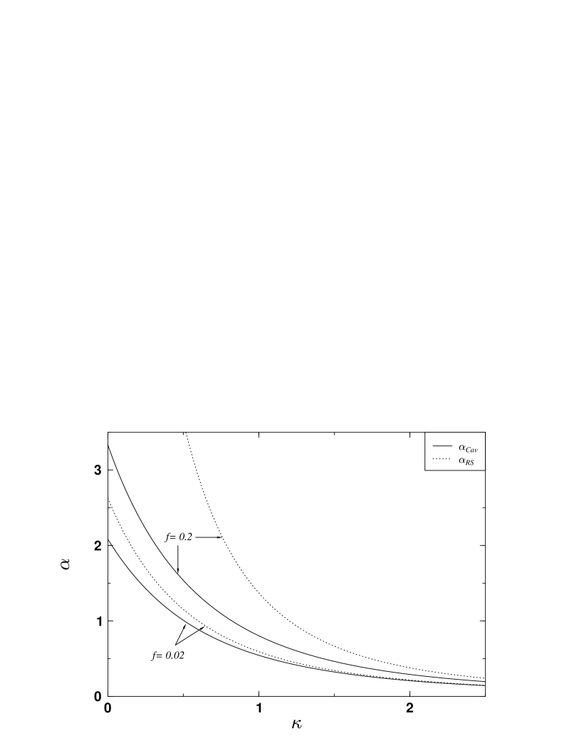
Figure 1: For two different error rates $f$ the storage capacity $\alpha$ is presented as a function of the stability $\kappa$ for both estimates (17) and (20).

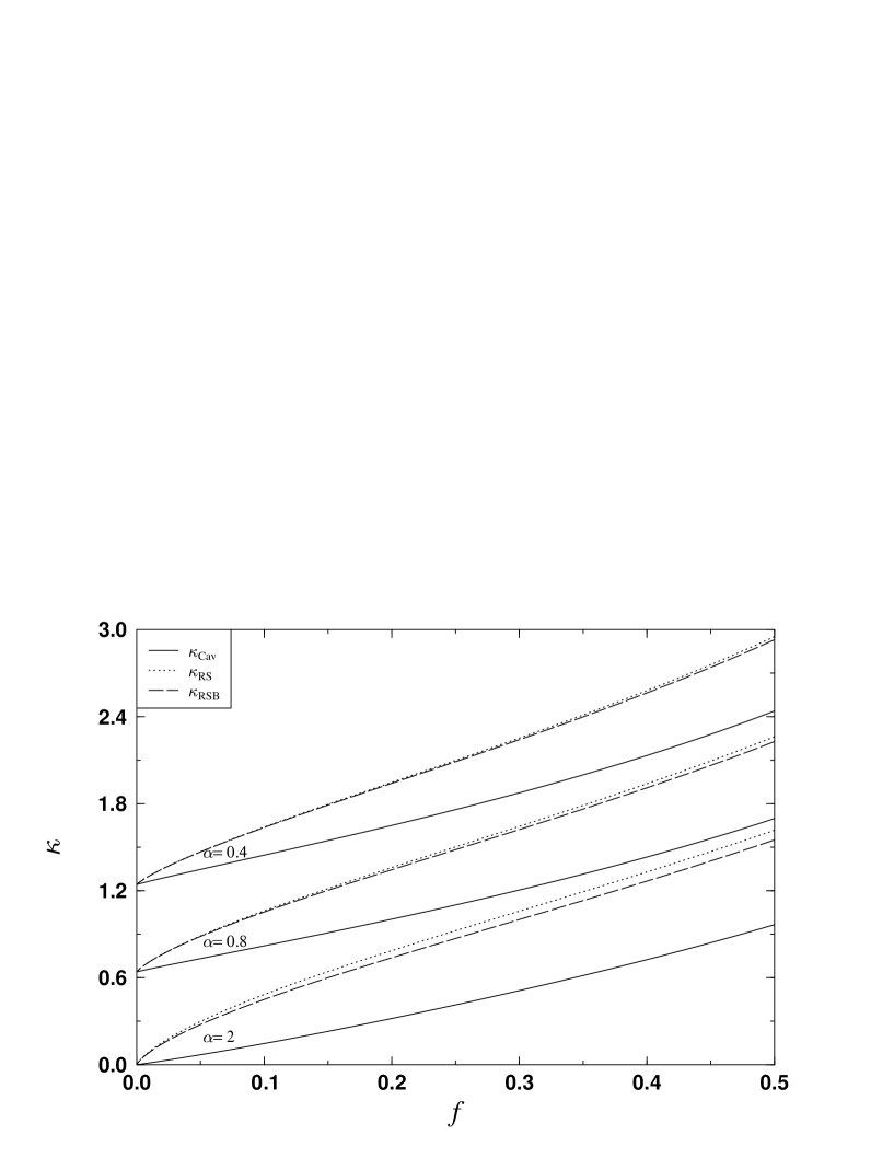
Figure 2: The stability $\kappa$ is presented as a function of the error rate $f$ for $\alpha=2.0$, 0.8 and 0.4. Results are shown for the cavity-method and the replica calculation in RS and 1-step-RSB approximation.

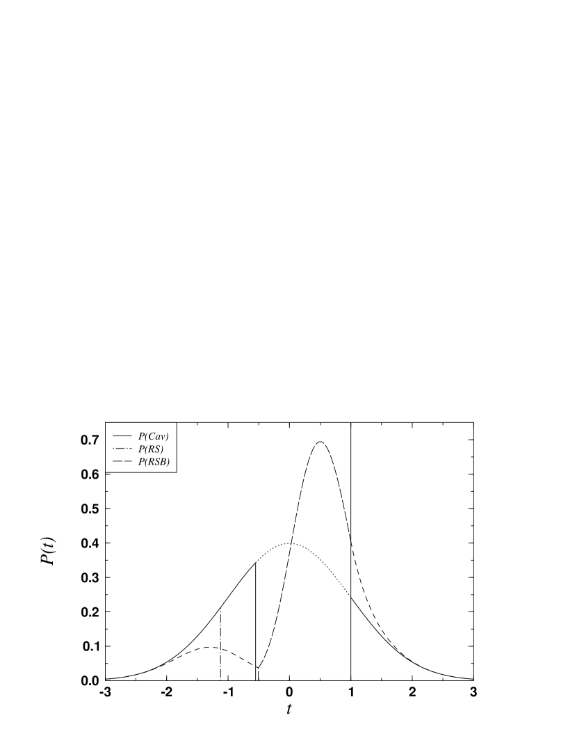
Figure 3: The probability density $P(t)$ of the local fields $t$ before learning is presented as a function of $t$ at $\alpha=1$ and $\kappa=1$. Again results are shown for the cavity-method and the replica calculation in RS and 1-step-RSB approximation. The distribution after training is given by pushing the middle segment to a $\delta$-Peak at $\kappa=1$ in every case. The cavity-method yields an error rate $f=0.29092$, the replica method gives $f=0.13073$ in RS and $f=0.13576$ in 1-step-RSB approximation. The fraction of explicitly learned patterns is 0.55042 for the cavity approximation and 0.71062 and 0.66745 respectively for the replica calculations.

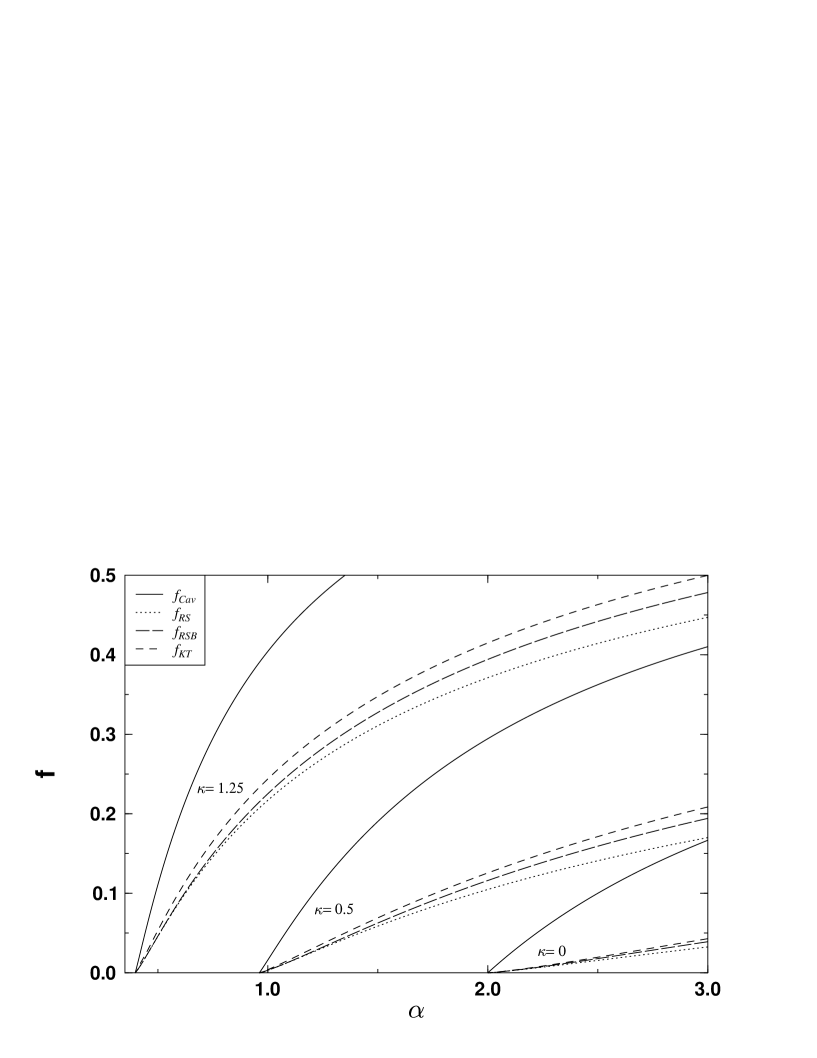
Figure 4: The error rate $f$ is presented as a function of $\alpha$ for $\kappa=1.25$, $0.5$ and $0$. The results are given for the cavity method, the RS and 1-step-RSB approximation as well as the result $f_{\hbox{\tiny KT}}$, which is calculated by putting together the Kuhn-Tucker conditions and the local fields of the RSB-solution. The best estimate is very likely between these RSB-graphs, i.e. $f_{\hbox{\tiny RSB}}$ and $f_{\hbox{\tiny KT}}$, and probably closer to $f_{\hbox{\tiny RSB}}$.

Figure 5: The AND-machine with tree structure (NRF). The weights between the intermediate layer and the output neuron are fixed. A threshold between 0 and 1 at the output-neuron takes care that there only is a positive output if both intermediate neurons are positive.

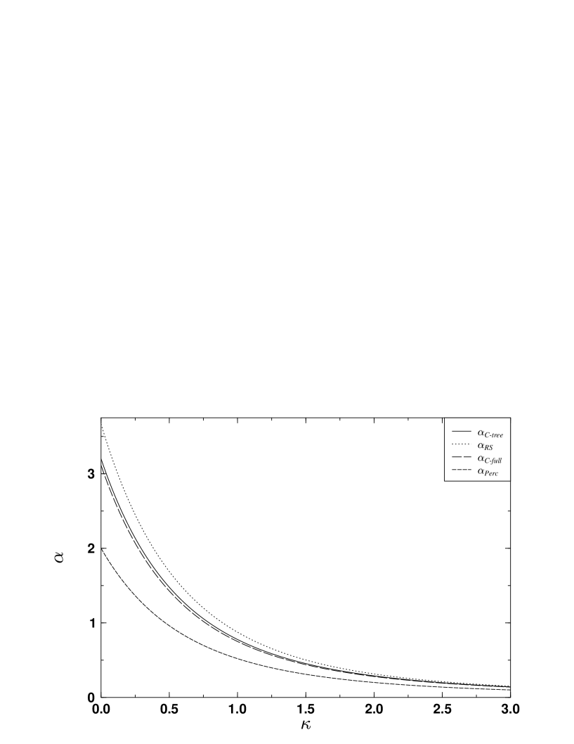
Figure 6: The storage capacity of the AND-machine is presented as a function of $\kappa$ for $b=0$. The results for the cavity method and for the replica calculation are given. The storage capacity $\alpha_{\hbox{\scriptsize full}}$ of the fully connected AND-machine, see 3.3, and $\alpha_{\hbox{\scriptsize Perc}}$ of the simple perceptron are presented for comparison

Figure 7: The overlap $R$ of both subnetworks of the fully connected AND-machine is presented as a function of the bias parameters $b$ from (24). The result for the cavity method gives a higher correlation of the subnetworks compared to Fig. 3.a in [17]. We have $R=0$ at $b=-1/3$, which means $\alpha_{-}=2\alpha_{+}$, in contrast to $R=0$ at $b=0$ in [17].

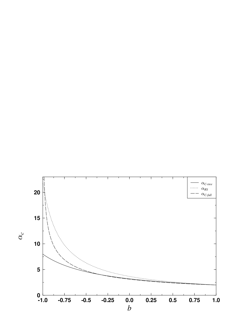
Figure 8: The maximal storage capacity of the AND-machine is presented as a function of the bias parameter $b$ from (24). The result of the cavity method for the tree structure is compared to the RS-result from [17] and the cavity result for the fully connected AND-machine. The largest deviations occur for small values of $b$. For the fully connected AND-machine the storage capacity is again smaller than with the replica calculation (see Fig. 3.b in [17]). We have $\alpha_{\hbox{\scriptsize C-full}}=\alpha_{\hbox{\scriptsize C-tree}}$ at $b=-1/3$, when $R=0$. For $b\to-1$ we have $\alpha_{\hbox{\scriptsize C-full}}\to\infty$ as in [17].

Figure 9: Table 1: The numbers $(n,k)$ of possible arrangements of $n$ letters with $k$ identities as described in the text. At the same time, these numbers are the coefficents of $\alpha_{\hbox{\scriptsize eff}}^{n-k}$ in the $n$th term on the r.h.s. of eqn.(51). In the main text it is shown, that the alternate sum along the diagonals – connected as a guide to the eye – disappears: $\sum_{l}(-1)^{l}(n+l,l)=0$. E.g. $1-3+2=0$, $1-6+10-5=0$ etc..

References

- [1] Gerl, F., Krey, U.: J. Phys. A 27, 7353 (1994)
- [2] Gerl, F., Krey, U.: J. Phys. A 28, 6501 (1995)
- [3] Winkel, J.Ó., Gerl, F., Krey, U.: Z. Physik B 100, 149 (1996).
- [4] Mézard, M., J. Phys. A 22, 2181 (1989)
- [5] Kinzel, W., Opper, M., Dynamics of Learning, in: Physics of Neural Networks, (L. van Hemmen, E. Domany and K. Schulten, eds.), Berlin, Heidelberg, New York, Springer 1991, p.149
- [6] Griniasty, M.: Phys. Rev. E 47, 4496 (1993)
- [7] Wong, K.Y.M.: Europhys. Lett., 30 (4), 245 (1995)
- [8] Gardner, E., Derrida, B.: J. Phys. A 21, 271 (1988)
- [9] Bouten, M.: J. Phys. A 27, 66021 (1994)
- [10] Griniasty, M., Gutfreund, H.: J. Phys. 24, 715 (1990)
- [11] Majer, P., Engel, E., Zippelius, A.: J. Phys. A 26, 7405 (1993)
- [12] Anlauf, J.K., Biehl, M.: Europhys. Lett. 10, 687 (1989)
- [13] Opper, M.: Phys. Rev. A38, 3824 (1988)
- [14] Fontanari, J.F., Theumann, W.K., J. Phys. bf A 26, L1233 (1993)
- [15] Whyte, W., Sherrington, D.: J. Phys. A 29, 3063 (1996)
- [16] Mézard, M., Parisi, G., Virasoro, M.A.: Spin glass theory and beyond, World Scientific, Singapore 1987
- [17] Griniasty,M., Grossman, T., Phys. Rev. A 45 8924 (1992)
- [18] Minsky, M.L., Papert, S.A., Perceptrons, MIT Press, Cambridge MA., 1969.
- [19] Mitchison, G.J, Durbin, R.M., Biol. Cybernetics 60 345 (1989)
- [20] Barkai, E., Hansel, D., Sompolinsky, H., Phys. Rev. A 45 4146 (1992)
- [21] Engel, A., Köhler, H.M., Tschepke, F., Vollmayr H., Zippelius, A., Phys. Rev. A 45 7590 (1992)
- [22] Wendemuth, A: Int. J. Neural Systems 5, 217 (1994)
- [23] Gardner, E.: Europhys. Lett. 4, 481 (1987)
- [24] Biehl, M., Anlauf, J.k., Kinzel, W., in: Neurodynamics, Eds. F. Pasemann and H.D. Doebner, World Scientific, Singapore 1991
- [25] Bernhart, F.R.: private communication
- [26] Hurwitz, A., Courant, R., Allgemeine Funktionentheorie und Elliptische Funktionen, 4th ed., Springer Verlag, Berlin,1964, p. 138
- [27] Biehl, M., PhD thesis, University of Giessen, 1992