Diffusion and localization in chaotic billiards

One of the main modifications that quantum mechanics introduces in our classical picture of deterministic chaos is “quantum dynamical localization” which results e.g. in the suppression of chaotic diffusive-like process which may take place in systems under external periodic perturbations. This phenomenon, first pointed out in the model of quantum kicked rotator [1], is now firmly established and observed in several laboratory experiments [2].

For conservative Hamiltonian systems the question of localization is much less investigated. The situation here is much more intriguing : from one hand, in a conservative system, one may argue that there is always localization due to the finite number of unperturbed basis states effectively coupled by the perturbation; on the other hand a large amount of numerical evidence indicates that quantization of classically chaotic systems leads to results which appear in agreement with the predictions of Random Matrix Theory (RMT) [3].

Recently the problem of localization in conservative systems has been explicitely investigated. In particular, on the base of Wigner band random matrix model, conditions for localization were explicitely given together with the relation between localization and level spacing distribution [4].

Billiards are very important models in the study of conservative dynamical systems since they provide clear mathematical examples of classical chaos and their quantum properties have been extensively studied theoretically and experimentally. Moreover they are becoming increasingly relevant for the study of optical processes in microcavities which may lead to possible applications such as the design of novel microlasers or other optical devices [5].

In this paper we focus our attention on a two dimensional chaotic billiard: the Bunimovich stadium, and study the classical diffusive process which takes place in angular momentum. This will allow us to predict the conditions for quantum localization and therefore the conditions under which the standard Random Matrix Theory is not applicable.

We consider the motion of a particle having mass $m$, velocity $\vec{v}$ and elastically bouncing inside the stadium shown in Fig 1. We denote with $R$ the radius of the semicircles and with $2a$ the length of the straight segments. The total energy is $E=m\vec{v}^{2}/2$.

The statistical properties of the billiard are controlled by the dimensionless parameter $\epsilon=a/R$ and, for any $\epsilon>0$, the motion is ergodic, mixing and exponentially unstable with Lyapunov exponent $\Lambda$ which, for small $\epsilon$, is given by [6] $\Lambda\sim\epsilon^{1/2}$.

For the analysis of classical dynamics, a typical choice of canonical variables is $(s,v_{t})$ where $s$ measures the position along the boundary of the collision point and $v_{t}$ is the tangent velocity. These variables however, are quite difficult to treat from the quantum point of view. For this purpose it is convenient instead to consider $l$, the angular momentum calculated with respect to the center of the stadium, and the angle $\theta$ which describes, together with $r(\theta)$, the position of the particle in the usual polar coordinates. It is important to stress that with this choice of variables, the invariant measure $d\mu=dsdv_{t}$ is preserved only to order $\epsilon$, that is $d\mu=dsdv_{t}=d\theta dl+o(\epsilon)$

At a given energy $E$, the angular momentum must satisfy the relation $|l|<l_{max}=(R+a)\sqrt{2Em}$. It is therefore convenient to introduce the rescaled quantity $L=l/l_{max}$. Then the classical motion takes place on the cylinder $0\leq\theta<2\pi$, $-1<L<1$.

It is expected that for $\epsilon<<1$ a diffusive process will take place in angular momentum with a diffusion coefficient $D=D(\epsilon)$. In order to obtain an estimate for $D(\epsilon)$ we now derive an explicit expression for the boundary map in the variables $(L,\theta)$. The change $\Delta L$ after a collision with the boundary can be easily obtained to order $\epsilon$, by neglecting collisions with straight lines and by taking into account that in the collision only the normal velocity $v_{n}=\vec{v}\cdot\vec{n}$ changes the sign. Here $\vec{n}\simeq\vec{e}_{r}+\epsilon\sin\theta sign(\cos\theta)\vec{e}_{\theta}$, $\vec{e}_{r}$ and $\vec{e}_{\theta}$ being the usual polar coordinates unit vectors. One then get :

$$\Delta L=\bar{L}-L=-2\epsilon\sin\theta sign(\cos\theta)sign(L)\sqrt{1-L^{2}}$$ (1)

On the other side the change in $\theta$, to zero order, is given by :

$$\Delta\theta=\bar{\theta}-\theta=\pi-2\arcsin({\bar{L}})$$ (2)

According to a standard procedure [7] we introduce a generating function $G(\bar{L},\theta)$ in such a way that the map defined by

$$L={{\partial G}\over{\partial\theta}};\qquad\bar{\theta}={{\partial G}\over{\partial{\bar{L}}}}$$ (3)

coincides with $\Delta L$ at first order in $\epsilon$ and with $\Delta\theta$ at zero-th order. The generating function is given by:

$$G(\bar{L},\theta)=(\theta+\pi){\bar{L}}-2\int^{\bar{L}}dL\arcsin L+\epsilon g(\bar{L})|\cos\theta|$$ (4)

where $g(\bar{L})=2sign(\bar{L})(1-{\bar{L}}^{2})^{1/2}.$ The generated (implicit) area–preserving map is

$$\begin{array}[]{l}\bar{L}=L-2\epsilon\sin\theta sign(\cos\theta)sign(\bar{L})(1-{\bar{L}}^{2})^{1/2}\\ \bar{\theta}=\theta+\pi-2\arcsin(\bar{L})+\epsilon g^{\prime}(\bar{L})|\cos\theta|\end{array}$$ (5)

By taking the local approximation in the angular momentum, the map (5) writes :

$$\begin{array}[]{l}\bar{L}=L-2\epsilon\sin\theta sign(\cos\theta)sign(\bar{L})\sqrt{1-L_{0}^{2}}\\ \bar{\theta}=\theta+\pi-2\arcsin(\bar{L})\end{array}$$ (6)

which remains area–preserving and can be easily iterated (here $L_{0}$ is the initial angular momentum).

The agreement of map (6) with the true dynamics can be numerically checked and it is shown in Fig.2 where we plot $L^{*}=(\bar{L}-L)/(2\epsilon\sqrt{1-L_{0}^{2}})$ against $\theta$. Points represent billiard dynamics while the full line is the function $f(\theta)=-\sin\theta sign(\cos\theta)$.

Notice that the function $f(\theta)$ is periodic of period $\pi$ and has a discontinuity at $\theta=\pi/2$. This gives to the map (6) a structure very close to the sawtooth map which is known[8] to be chaotic and diffusive with a diffusion rate $D$ which, for small values of the kick strength $\epsilon$, is given by $D\sim\epsilon^{5/2}$. This behaviour, according also to our numerical computations, appears to be generic for maps which have such type of discontinuity.

We may proceed now to a numerical investigation of the diffusive process. To this end we consider a distribution of particles with given initial $L_{0}$ and random phases $\theta$ in the interval $(0,2\pi)$ and integrate the classical equations of motion inside the billiard. In Figs. 3a,b we present the behaviour of $\Delta L^{2}=\langle L^{2}\rangle-\langle L_{0}\rangle^{2}$ as a function of the number of collisions $n$ and the distribution function $f_{n}(L)$ at fixed $n$ as a function of $(L-L_{0})$. As it is seen, $\Delta L^{2}$ grows diffusively and the distribution function is in good agreement with a Gaussian[9]. In particular the dependence $D=D(\epsilon)$ of the diffusion coefficient can be easily computed and the result $D=D_{0}\epsilon^{5/2}$ (see Fig.4) is in agreement with predictions of map (6) with $D_{0}=1.5$.

The analysis of the classical diffusive process allows to make some predictions concerning the quantum motion and in particular to estimate the conditions under which the quantum localization phenomenon will take place [10]. First of all, in order that any quantum diffusive process may start it is necessary to be above the perturbative regime. In particular the level number must be sufficiently high so that the De Broglie wavenumber $k$ of the corresponding wavefunction must satisfy the relation $k>1/a$. This implies $E>E_{p}=\hbar^{2}/2ma^{2}$ which is the energy necessary to confine a quantum particle inside a box of length $a$. Using the well known Weyl formula for the total number of states with energy less than $E$ [3]

$$\langle N(E)\rangle\approx{{m\cal{A}}\over{2\pi\hbar^{2}}}E\approx{1\over 8}m\left({R\over\hbar}\right)^{2}E$$ (7)

where ${\cal A}$ is the area of a quarter of billiard, and keeping only the leading term, we obtain that in order to be in a non perturbative regime we have to consider level numbers

$$N\gg N_{p}\simeq{{1}\over{16\epsilon^{2}}}$$ (8)

We call $N_{p}$ perturbative border.

According to the well known arguments [11], above the perturbative border (8) quantum diffusion in angular momentum takes place with a diffusion coefficient close to the classical one. This diffusion proceeds up to a time $\tau_{B}\sim D_{eff}/\hbar^{2}$ after which diffusion will be suppressed by quantum interference. This time is related to the uncertainty principle. Namely, for times less than $\tau_{B}$ the discrete spectrum is not resolved and the quantum motion mimics the classical diffusive motion [11, 12]. Here $D_{eff}=D_{0}\epsilon^{5/2}2mER^{2}$ is the classical diffusion coefficient in real (not scaled) angular momentum.

The nature of the quantum steady state will depend crucially on the ergodicity parameter [12]

$$\lambda^{2}={{\tau_{B}}\over{\tau_{E}}}$$ (9)

where $\tau_{E}=l^{2}_{max}/D_{eff}\simeq 2mER^{2}/D_{eff}$ is the ergodic relaxation time.

For $\lambda\ll 1$ the quantum steady state is localized while for $\lambda\gg 1$ we have quantum ergodicity. The critical value $\lambda=1$ leads to $l_{max}\hbar=D_{eff}$ that is $E=E_{erg}=\epsilon^{-5}D_{0}^{-2}\hbar^{2}/2mR^{2}$. We then have :

$$N=N_{erg}\simeq{{1}\over{16D_{0}^{2}\epsilon^{5}}}$$ (10)

It follows that only for $N>N_{erg}$ there is quantum ergodicity and therefore one expects statistical properties of eigenvalues and eigenfunctions to be described by RMT. Instead for $N<N_{erg}$, even if $N\gg N_{p}$, namely very deep in quasiclassical regions, statistical properties will depend on parameter $\lambda=D_{0}\sqrt{8N\epsilon^{5}}$ and not separately on $\epsilon$ or $N$. For example, the nearest neighbour levels spacing distribution $P(s)$ will approach $e^{-s}$ when $\lambda\ll 1$.

We have tested this prediction by numerically computing the level spacing distribution for different values of $\epsilon$ and $N$. One example is shown in Fig.5 for which $N\gg N_{p}$ but since $\lambda\ll 1$ the distribution $P(s)$ is close to $e^{-s}$ as expected. Similar behaviour is expected for other quantities such as the two points correlation function, the probability distribution of eigenfunctions, etc. The numerical computations are based on the improved plane wave decomposition method[13]. The accuracy of eigenvalues is better than one percent of the mean level spacing. We also compared the results with the semiclassical formula in order to check that there are no missing levels.

Notice that the effect predicted here is entirely due to quantum dynamical localization and bears no relation with the existence of bouncing ball orbits. The same behaviour will be present in chaotic billiards in which no family of periodic orbits exists.

The effects of quantum localization discussed here should be observable in microwave or sound wave experiment. Finally we would like to mention that the diffusive process in angular momentum and the corresponding suppression caused by quantum mechanics may be of interest for a new class of optical resonators which have been recently proposed [5].

We are indebted to R.Artuso, B.V.Chirikov, I.Guarneri and D.Shepelyansky for valuable discussions and suggestions. B. Li is grateful to the colleagues of the University of Milano at Como for their hospitality during his visit. His work is supported in part by the Research Grant Council RGC/96-97/10 and the Hong Kong Baptist University Faculty Research Grant FRG/95-96/II-09 and FRG/95-96/II-92.

*

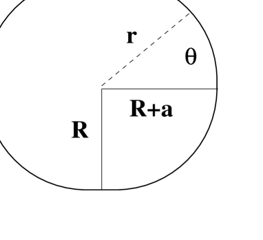
FIG. 1.: The Bunimovich stadium with radius $R$ and straight segments $2a$ ; the variables $(r(\theta),\theta)$ indicate the position of the point along the boundary.

*

FIG. 2.: Comparison between the billiard dynamics and the map $(6)$. Here we plot the variable $L^{*}$ versus $\theta$ (see text). Points are obtained from numerically integrating the motion of one particle in the billiard for $100$ iterations, starting from $L_{0}=0$ and a random position along the boundary, while the full line is the function $f(\theta)$ (see text). Here $\epsilon=0.01$. The points not belonging to the curve are due to collisions with one of the straight lines; this occurrence is outside the approximation of map $(6)$.

*

FIG. 3.: Diffusion in angular momentum for the billiard with $\epsilon=0.01$. Here an ensemble of $10^{4}$ particles was chosen with initial $L_{0}=0$ and random position along the boundary. a) $\Delta L^{2}$ as a function of the number of collisions $n$; the dashed line is the best fit and gives $D=\Delta L^{2}/n=1.5\cdot\quad 10^{-5}$. b) Distribution function after $n=500$ collisions averaged over the last 50 collisions. The full line is the best fitting Gaussian with average $-0.016$ and variance $0.1$.

*

FIG. 4.: Diffusion coefficient $D=\Delta L^{2}/n$ for the stadium (full circles) as a function of $\epsilon$. Open circles indicate the diffusion rate obtained from the map (6). The line is obtained by the usual best fitting procedure to the true dynamics (full circles) and gives $D=D_{0}\epsilon^{2.5}$ with $D_{0}=1.5$.

*

FIG. 5.: Level spacings distribution computed on $2000$ levels in the interval $51000<N<53000$ for $\epsilon=0.01$ (a) and $\epsilon=0.1$ (b). In the first case (a) $N_{p}\simeq 600$ and $N_{erg}\simeq 2.8\cdot 10^{8}$ and therefore $N_{p}\ll N\ll N_{erg}$. The value $\lambda\simeq 0.01$ of the ergodicity parameter accounts for the fact that the numerically computed $P(s)$ is close to $e^{-s}$ (full curve). In the case (b) one has $N_{erg}\simeq 2.8\cdot 10^{3}\ll N$ and therefore, as expected, the distribution $P(s)$ is close to Wigner-Dyson (dotted curve).

REFERENCES

- [1] G.Casati, B.V.Chirikov, J.Ford and F.M.Izrailev, Lectures Notes in Physics 93 (1979) 33, Springer Verlag ( see also Ref. 12 ).
- [2] E. J. Galvez, B. E. Sauer, L. Moorman, P. M. Koch and D. Richards, Phys. Rev. Lett. 61, (1988) 2011; J.E.Bayfield, G.Casati, I.Guarneri and D.Sokol Phys. Rev. Lett. 63, (1989) 364; M.Arndt, A.Buchleitner, R.N.Mantegna, H.Walther Phys. Rev. Lett. 67, (1991) 2435; F.L.Moore, J.C. Robinson, C.F.Bharucha, B.Sundaram and M.G.Raizen Phys. Rev. Lett. 75, (1995) 4598.
- [3] O.Bohigas, Proceedings of the 1989 Les Houches Summer School on “Chaos and Quantum Physics”, ed. M.J.Giannoni, A.Voros and J.Zinn-Justin, p.89, Elsevier Science Publisher B.V., North–Holland, (1991)
- [4] G.Casati, B.V.Chirikov, I.Guarneri and F.M.Izrailev Phys.Rev.E 48, (1993) R1613; G.Casati, B.V.Chirikov, I.Guarneri and F.M.Izrailev preprint Budker INP 95-98 Novosibirsk, (1995).
- [5] J.U.Nockel and A. D. Stone in Optical Processes in Microcavities, edited by R. K. Chang and A. J. Campillo (World Scientific Publishing Co., 1995), and A.Mekis, J.U.Nöckel, G.Chen, A.D.Stone and R.K.Chang, Phys. Rev. Lett. 75, (1995) 2682. In these papers it is proposed that the spoiling of high-Q whispering gallery modes in deformed dielectric spheres can be understood as a transition to chaotic ray dynamics (in deformed circular billiards) which can no longer be confined by total internal reflection.
- [6] G.Benettin, Physica 13D, (1984) 211.
- [7] A.J.Lichtenberg and M.A.Lieberman, Regular and Stochastic Motion, Applied Math. Series 38 (1983).
- [8] I.Dana, N.W.Murray and I.C.Percival Phys.Rev.Lett. 62 (1989) 233.
- [9] It may be interesting to remark that the diffusion coefficient computed in terms of the number of collisions, appears to depend on the initial value of angular momentum . This is due to the fact that the mean free path depends on angular momentum and that even though the system is ergodic, ergodicity is not uniform in time. If one computes the diffusion coefficient in terms of real physical time then the dependence on the initial value disappears. For the above reasons map (6) approximate the real dynamics provided is not too close to .
- [10] B.V.Chirikov preprint 90-116 Novosibirsk, (1990).
- [11] B.V.Chirikov, F.M.Izrailev and D.L.Shepelyansky, Sov. Scient. Rev. 2C, 209 (1981).
- [12] G.Casati and B.V.Chirikov , ”Quantum Chaos”, Cambridge University press, (1995); Physica D, 86 (1995) 220.
- [13] E.Heller, in Proceeding of the 1989 Les Houches Summer School on ”Chaos and Quantum Physics”, ed. M. Giannoni, A.Voros, J.Zinn-Justin, B.Li and M.J.Robnik J.Phys. A 27 (1994) 5509, and E.Vergini and M.Saraceno, Preprint 1994, ”Calculation by scaling of highly excited states of billiards”
*
*
*
*
*