Multifractality beyond the Parabolic Approximation: Deviations from the Log-normal Distribution at Criticality in Quantum Hall Systems

Abstract

Based on differences of generalized Rényi entropies nontrivial constraints on the shape of the distribution function of broadly distributed observables are derived introducing a new parameter in order to quantify the deviation from lognormality. As a test example the properties of the two–measure random Cantor set are calculated exactly and finally using the results of numerical simulations the distribution of the eigenvector components calculated in the critical region of the lowest Landau–band is analyzed.

Numerical simulations of disordered critical systems always face the problem of dealing with system sizes smaller then the relevant length scale therefore highly complex fluctuations appear. Consequently expectation values of observables do not represent the full picture for the description of the dynamics and physics involved, instead the whole distribution function of these observables should be studied. This problem has become the central issue of theoretical research over the past decade [1, 2, 3, 4].

Multifractal analysis [5] has now become a standard tool to handle the aforementioned fluctuations arising near criticality. Especially the disorder induced localization-delocalization (LD) transition is an important and widely studied example of such critical systems [6].

The general method of multifractal analysis starts with the calculation of the measure $Q(\ell)$ of the observable over boxes of linear size $\ell$ in a system of length $L$ divided into $M$ pieces of these boxes. In the thermodynamic limit of $\ell/L\to 0$ the $q$th moment of this distribution scales with a nontrivial exponent $D_{q}$ that is, in general, strongly $q$–dependent. These moments are often called as generalized inverse participation numbers (IPN). The quantity $(q-1)D_{q}$, also known as the mass exponent $\tau_{q}$, is a monotonous, nonlinear function of $q$.

Another way of describing these fluctuations is using the $f(\alpha)$ function, the Legendre–transform of $\tau_{q}$. The $f(\alpha)$ is a smooth, single–humped, concave function. It is the distribution of the exponents $\alpha_{q}=d\tau/dq$ that characterize the $\mu_{q}(\ell)\sim(\ell/L)^{\alpha_{q}}$ scaling of the box–observables where $\mu_{q}(\ell)$ is the total measure of the $q$th power of the observables $Q$ over the boxes with linear length $\ell$. The $f(\alpha_{q})$ gives the scaling of the number of boxes with measure $(\ell/L)^{\alpha_{q}}$ in the interval $(\alpha,\alpha+d\alpha)$

$$\rho(t,\alpha)=g(t,\alpha)e^{t\,f(\alpha)}$$ (1)

where we have introduced the variable $t=-\ln(\ell/L)$. The above distribution describes the multifractal in the sense that $\ln\rho(t,\alpha)/t\to f(\alpha)$ if $t\to\infty$. The $f(\alpha)$ function obeys certain general rules: $f^{\prime}(\alpha_{q})=q$, where prime denotes derivation with respect to $\alpha$. For some specific values of $q$

$$f^{\prime}(\alpha_{0}) = 0,\qquad f(\alpha_{0})=D_{0}$$ (3)

$$f^{\prime}(\alpha_{1}) = 1,\qquad f(\alpha_{1})=\alpha_{1}=D_{1}$$ (4)

where $D_{0}$ is the Hausdorff–dimension of the support of the observable $Q$. Furthermore the support of the $f(\alpha)$ spectrum is a finite interval [$\alpha_{-\infty},\alpha_{+\infty}$], and at the two limiting values the derivative of the $f(\alpha)$ is infinite. The importance of the study of the function $f(\alpha)$ is enhanced due to its connection to the properties of the local distribution function of the $Q$ variables as [6]

$$\Pi(t,\ln Q)\sim\exp[t(D_{0}-f(\alpha))],\qquad\alpha=\ln Q/t$$ (5)

The shape of the $f(\alpha)$ curve is close to a parabola [6, 8] which means that the distribution $\Pi(t,\ln Q)$ is a Gaussian and the $\Pi(t,Q)$ is lognormal. Therefore any deviation from the parabolic approximation (PA) shows up as a deviation of $\Pi(t,Q)$ from lognormality. Numerical experiments show that there is a substantial deviation of the distribution function (5) from the simple Gaussian especially for large values of $\ln Q$, hence it is even asymmetrical [7] (see Fig. 1).

The calculation of $f(\alpha)$ and $D_{q}$ functions in numerical experiments suffers from several difficulties. First this analysis is suitable only if $\ell\ll L<\xi$ is satisfied, where $\xi$ is the localization length and still the box–length should be larger that any microscopic length scale of the system. Second, higher moments of the distribution, $|q|>3$ are usually calculated with low precision and the PA is usually satisfactory. The PA is fixed by the values of $\alpha_{0}$ and $D_{0}$. In spite of the simplicity of the PA it breaks down at values of $q$ where the monotonicity of the $\tau_{q}$ is lost.

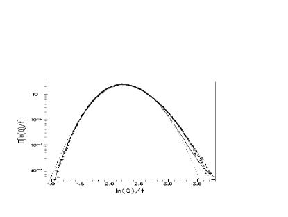
FIG. 1.: The joint probability distribution function of the local amplitudes $Q=|\psi|^{2}$ of the eigenstates taken in the critical region in a Quantum Hall System. The dashed line represents the parabolic approximation, the solid one is the improvement given in the text.

Apart from the results of numerical simulations, recently it has been shown analytically that the moments of the distribution function of the eigenstate components in a two dimensional disordered system shows multifractality [9], however, only the PA has been derived. In another work the multifractal properties of a relativistic fermion moving in a two dimensional random vector potential field has been derived [10] without the restrictions of the PA. Therefore it seems to be of growing importance of deriving as much information from numerical experiments as possible.

In this Letter we show that the deviations from the simple lognormal distribution can be measured with the application of specific Rényi–entropies [11]. These Rényi entropies are proportional to the variable $t$ only for strictly self–similar observables in the thermodynamic limit, e.g. deterministic multifractals such as the two–measure Cantor set, however, they are connected to some specific values of the scaling dimensions of the generalized IPNs and hence impose new conditions on the shape of the $f(\alpha)$ function.

Hereby we use two differences of Rényi entropies [11]. The first one describes the deviation of the generalized IPN $\ln P_{2}$ of the distribution Eq. (1) from the Shannon entropy $H$ (a special Rényi entropy) and the other one is the normalized value of $\ln P_{2}$

$$S_{2}=H-\ln P_{2}\quad{\rm and}\quad m_{2}=\ln M-\ln P_{2}$$ (6)

Generalizations for higher moments are also possible [17], however, numerical simulations for such cases are presently not too reliable. The above two parameters have already been successfully applied in a number of systems [12, 14, 15] for the shape–analysis of the complex distribution function of eigenvector components and energy spacing distributions.

The calculation of the quantities $S_{2}$ and $m_{2}$ involve integration over the measure of the distribution in question. In our case, we have to perform integration of Eq. (1) over the allowed range of the $\alpha$ values [$\alpha_{-\infty},\alpha_{+\infty}$]

$$P_{2}^{-1}(\ell) \sim \int_{\alpha_{min}}^{\alpha_{max}}\ell^{2\alpha}\rho(\ell,\alpha)d\alpha$$ (8)

$$H(\ell) \sim -\ln\ell\int_{\alpha_{min}}^{\alpha_{max}}\alpha\ell^{\alpha}\rho(\ell,\alpha)d\alpha$$ (9)

Furthermore, being interested only in the small $\ell$, i.e. large $t$ limit, we can apply an asymptotic method due originally to Laplace [16] and obtain an expansion of $t$ of the form [17]

$$S_{2}(t) = (D_{1}-D_{2})t+\sum_{k=0}^{\infty}s_{2,k}t^{-k}$$ (11)

$$m_{2}(t) = (D-D_{2})t+\sum_{k=0}^{\infty}m_{2,k}t^{-k}$$ (12)

From Eqs. (Multifractality beyond the Parabolic Approximation: Deviations from the Log-normal Distribution at Criticality in Quantum Hall Systems) it is clear that their ratio tends to a constant as $t\to\infty$

$$\gamma_{2}=\lim_{t\to\infty}{{S_{2}(t)}\over{m_{2}}(t)}={{D_{1}-D_{2}}\over{D_{0}-D_{2}}}.$$ (13)

This is the key result of our Letter. The $D_{1}$ and $D_{2}$ values in Eqs. (Multifractality beyond the Parabolic Approximation: Deviations from the Log-normal Distribution at Criticality in Quantum Hall Systems,13) are related to the $f(\alpha)$ function, since (4) $\alpha_{1}=f(\alpha_{1})=D_{1}$ and $D_{2}=2\alpha_{2}-f(\alpha_{2})$. On the other hand one can calculate the quantities $S_{2}/m_{2}$ directly using the observable $Q$ at any length scale. The latter value imposes a further condition on the $f(\alpha)$ through the dimensions $D_{1}$ and $D_{2}$ using relation Eq. (13): $f(\alpha_{2})=2\alpha_{2}-(\alpha_{1}-\gamma_{2}D_{0})/(1-\gamma_{2})$. Note that for a lognormal distribution $\gamma_{2}=1/2$ independently of the details of the distribution as it is also $\gamma_{2}=1/2$ for a parabolic $f(\alpha)$, hence a deviation from the value 1/2 is a sign of non-lognormal distribution and non-parabolic $f(\alpha)$ [13]. Furthermore, the denominator of Eq. (13) is the quantity that has been recently connected to the anomalous diffusion exponent by Refs. [8] and [18].

As an illustration first let us consider the two-measure Cantor set representing a binary process [5]. In this construction one divides the $[0,1]$ interval into two equal parts receiving different, $p$ and $1-p$ measures. While iterating this procedure for each subhalf of the interval we get a multifractal in $D_{0}=1$. This is a strictly selfsimilar multifractal if we keep the $0\leq p\leq 1/2$ value fixed, because for the $n$th stage $S_{2}^{(n)}=n\,S_{2}^{(1)}$ and $m_{2}^{(n)}=n\,m_{2}^{(1)}$ where $S_{2}^{(1)}$ and $m_{2}^{(1)}$ are the values for the initial configuration. Hence all the $s_{2,n}$ and the $m_{2,n}$ in Eq. (Multifractality beyond the Parabolic Approximation: Deviations from the Log-normal Distribution at Criticality in Quantum Hall Systems) are zero, and the $\gamma_{2}$ quantity is independent of $n$ and is a function of $p$ [17].

Next we consider a generalization of this Cantor set by choosing at every stage a different value for $p_{n}$ then we obtain a non–selfsimiliar multifractal the random binary Cantor set (RBCS). It is straightforward to derive the $f(\alpha)$ function once the distribution function of the $p_{n}$ sequence is further specified. Taking a uniform distribution over the interval $[1/2-\delta,1/2+\delta]$ we have found that $\gamma_{2}(\delta)$ is a smooth function of $0\leq\delta\leq 1/2$. Using this simple mathematical construction we will show that the PA can be easily improved with the application of parameter $\gamma_{2}$ Eq. (13). As an example we took $\delta=1/3$. The PA in Fig. 2 is denoted as a dotted line while the exact relation is represented by the solid symbols. We can see that adding a fourth order term $(\alpha-\alpha_{0})^{4}$ to the PA fulfilling both Eqs. (1) and (13) in $f(\alpha)$ gives the solid line that is clearly a much better approximation than the simple PA.

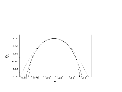
FIG. 2.: The distribution of the random binary Cantor set (RBCS) with $\delta=1/3$. The dashed line stands for the parabolic approximation and the solid one is the fourth order one using parameter $\gamma_{2}$ (see. Eq. (13)). The symbols represent the exact relation.

Finally we will apply our analysis to the widely studied LD transition that takes place in a two dimensional disordered system subject to a perpendicular strong magnetic field: the quantum Hall system [6, 19]. This LD transition is responsible to the integer quantum Hall effect. It is described by the critical index $\nu$ of the localization length and the $f(\alpha)$ spectrum, that is believed to be universal [6], however, up to now the focus has been set on the PA only and the value of $\alpha_{0}$ fixing the position of the maximum of it. The value of $\alpha_{0}$ describes the scaling behavior of the typical local electron density. We show how the deviation from the lognormal distribution can be measured using Eq. (13) and propose an optimal modification of both the $f(\alpha)$ and the distribution function $\Pi(t,\ln Q)$. For that purpose we have performed calculations of two dimensional systems of linear size of 200 magnetic lengths. We have obtained 134 eigenfunctions and calculated the overall joint probability distribution function of the local amplitudes $Q=|\psi|^{2}$. In Fig. 1 we have plotted the logarithm of the histogram of $\ln Q$ as a function of $\ln Q/t$. On the same figure the PA is also presented. The discrepancy is clear especially for larger values of $Q$. On the same figure we have given a possible improvement of the analytical $f(\alpha)$ that shows a much better resemblance to the numerical data.

FIG. 3.: Scaling dependence of parameters $m_{2}(t)/t$ and $S_{2}(t)/t$ as a function of $1/t$. Solid symbols stand for the values obtained in the Quantum Hall System and continuous curves show several [$K/L$] order Padé approximants: dashed line [0/2], dotted line [0/3] and solid line [0/4].

The improvement in Fig. 1 was achieved similarly as for the case of the RBCS. For that purpose we have calculated the $m_{2}(t)/t$ and $S_{2}(t)/t$ values and plotted as a function of $1/t$. Unfortunatelly the low system size is a severe limitation on our problem, since it is desired to obtain the values of $m_{2}(t)/t$ and $S_{2}(t)/t$ for $t\to\infty$. However, it is not possible to go beyond $t_{max}=\ln L$ and current computation possibilities impose a limit of $t_{max}\approx 6.0$. In order to obtain an acceptable value for the values $m_{2}(t)/t$ and $S_{2}(t)/t$ as $1/t\to\infty$ we have performed an [$K/L$] order Padé approximation [20] for both quantities. Besides finite size scaling this type of approximation is ready to give an estimate of the coefficients in the expansions Eq.(Multifractality beyond the Parabolic Approximation: Deviations from the Log-normal Distribution at Criticality in Quantum Hall Systems). Not having data obtained for different system sizes at hand we can show that the Padé approximation indeed gives acceptable results, as well. We assumed that the [$K/L$] order approximation should have no singularity in the given interval and has to fall to zero for $1/t\to\infty$ since on the scale $\ell\approx L$ the distribution is homogeneous, thus reducing to the possibilities to $K<L$ and $K=0$. In Fig. 3 we have plotted the calculated quantities together with several Padé approximants. The limit $1/t\to 0$ gives the approximate value for the parameter $\gamma_{2}$. This way we obtained 0.445 for [0/2] 0.439 for [0/3] and 0.436 for [0/4]. Therefore we set the value of $\gamma_{2}\approx 0.44$. On the other hand, using standard multifractal analysis, our data gives $\alpha_{0}=<\ln Q>/t=2.24$, $D_{1}=1.78$ $D_{2}=1.61$ that are all well in the generally accepted range [6, 19]. The latter values yield $\gamma_{2}\approx 0.44$ again.

Having $\alpha_{0}$ and $\gamma_{2}$ at hand we may extend the functional form of $f(\alpha)$ beyond the PA in order to get a better aggreement with the numerical distribution function (see Eq. (5)). For the improvement of the functional form of the $f(\alpha)$ entering in Eq. (5) there should be a number of possibilities. We used the addition of the term $(\alpha-\alpha_{0})^{3}$ and $(\alpha-\alpha_{0})^{5}$ to the PA fixing their coefficients requiring the constraints Eqs. (1) and (13) within an error of 10^-4. Therefore the $\Pi(x)$ function seems to be modified as $\Pi(x)=\Pi_{\rm PA}(x)\,\exp[-t(c_{3}x^{3}+c_{5}x^{5})]$ where $x=\ln Q/t-\alpha_{0}$, $c_{3}\approx-0.03$ and $c_{5}\approx 0.12$.

In this Letter we have introduced the differences of Rényi entropies in order to describe the behavior of any multifractal as a function of $t=-\ln(\ell/L)$. These parameters enable to look beyond the parabolic approximation and obtain further constraints on the shape of the $f(\alpha)$ function as well as the distribution function of the multifractal quantity. In order to get insight in the $t$ dependence we have applied Laplace’s method and tried the results on exactly known deterministic and random multifractals. In the former case the self similarity property is also obtained while the latter case was a good test how the improvement from PA can be done.

Finally we have analyzed the joint distribution function of the local amplitudes of wave functions calculated in the critical regime of the Quantum Hall System. We have applied the Padé approximation in order to mimic the thermodynamic limit. The results show a possible tail of the distribution function that is irregular for smaller amplitudes.

Acknowledgements One of the authors (I.V.) is grateful for the warm hospitality at the Institut für Theoretische Physik, Universität zu Köln where part of this work has been completed. Financial support from Országos Tudományos Kutatási Alap (OTKA), Grant Nos. T7238/1993 and T014413/1994 is gratefully acknowledged.

REFERENCES

- [1] Y. Imry, 1986 Europhys. Lett. 1 249, (1986).
- [2] B. L. Altshuler, V. E. Kravtsov, and I. V. Lerner, Phys. Lett. 134A 488, (1989).
- [3] J. B. Pendry, A. MacKinnon, and A. B. Pretre, Physica 168 400, (1990).
- [4] B. L. Altshuler, P. A. Lee, and R. A. Webb eds., Mesoscopic Systems (North Holland, Amsterdam, 1991).
- [5] B. Mandelbrot: Fractals: Form, Chance and Dimension (W. H. Freedman, San Francisco, 1977); T. C. Halsey, M. H. Jensen, L. P. Kadanoff, I. Procaccia, and B. Shrainman, Phys. Rev. A 33 1141, (1986).
- [6] For a review see M. Janssen, Int. J. Mod. Phys. B 8, 943, (1994).
- [7] S. N. Evangelou, J. Phys. A.: Math. Gen. 23, L317 (1990).
- [8] W. Pook and M. Janssen, Z. Phys., 82, 295, (1991).
- [9] V. I. Fal’ko and K. B. Efetov, Europhys. Lett. 32, 627, (1995); Phys. Rev. B 52, 17413 (1995), see references for earlier studies.
- [10] C. de C. Chamon, Ch. Mudry, X.-G. Wen, preprint cond-mat/9510088; J. S. Caux, I. I. Kogan, and A. M. Tsvelik, Nucl. Phys. B 466, 444 (1996).
- [11] A. Rényi, Selected Papers (Akadémiai Kiadó, Budapest, 1976) p. 526.
- [12] J. Pipek and I. Varga, Phys. Rev. A 46 3148, (1992).
- [13] I. Varga, Ph. D. Thesis, Technical University of Budapest (1993), unpublished.
- [14] J. Pipek and I. Varga, Int. J. Quantum Chem. 51 539, (1994).
- [15] I. Varga, E. Hofstetter, M. Schreiber, and J. Pipek, Phys. Rev. B 52 7283, (1995).
- [16] A. Erdélyi, Asymptotic expansions (Dover, New York, 1956), p. 36; N. G. Bruijn, Asymptotic methods in Analysis (North Holland, Amsterdam, 1958), p. 60.
- [17] J. Pipek and I. Varga, Intern. J. of Quantum Chem., in press
- [18] J. T. Chalker, Physica A 176 253 (1990).
- [19] M. Janssen, O. Viehweger, U. Fastenrath and J. Hajdu, Introduction to the Theory of the Integer Quantum Hall Effect (VCH, Weinheim, 1994); B. Huckestein, Rev. Mod. Phys. 67, 357 (1995).
- [20] G. A. Baker, Jr. and P. Graves-Morris: Padé Approximants, Part I: Basic Theory (Addison-Wesley, London, 1981).