Simulation studies of fluid critical behaviour

Abstract

We review and discuss recent advances in the simulation of bulk critical phenomena in model fluids. In particular we emphasise the extensions to finite-size scaling theory needed to cope with the lack of symmetry between coexisting fluid phases. The consequences of this asymmetry for simulation measurements of quantities such as the particle density and the heat capacity are pointed out and the relationship to experiment is discussed. A general simulation strategy based on the finite-size scaling theory is described and its utility illustrated via Monte-Carlo studies of the Lennard-Jones fluid and a two-dimensional spin fluid model. Recent applications to critical polymer blends and solutions are also briefly reviewed. Finally we consider the outlook for future simulation work in the field.

I Introduction

That the vapour pressure curve of a simple fluid terminates in a critical point has been known since the latter half of the last century when Andrews demonstrated the phenomenon of critical opalesence in carbon dioxide [1]. Shortly afterwards, van der Waals published a mean field type theory of liquid-vapour coexistence that predicted the existence of a critical point with divergent compressibility, and formed much of the basis of the understanding of the critical region for many years thereafter. Arguably, however, the modern era of critical phenomena began in the 1940s, when Guggenheim realised that the coexistence curves of many simple fluids are not in fact parabolic as predict by van der Waals theory, but nearly cubic. At around the same time, Onsager published his famous solution to the 2D ferromagnetic Ising model, which among other things allowed it to be demonstrated that the critical exponents are strongly non-classical. It was not until the 1960s, however, that activity in the field really began to take off. Accurate experimental studies of magnetic systems on the one hand, and series expansion studies of model spin systems on the other, providing vivid illustration of the phenomena of scaling and universality, already hinted at previously by Guggenheim for fluids [2]. These findings heralded the beginning of a prodigious effort to understand more deeply the nature of critical phenomena, and in particular of finding ways of dealing with the profusion of length scales that characterise the critical region and which underpin the singularities in physical observables that are its hallmark. Milestones in this quest to date, are the renormalisation group [3] and conformal invariance theories [4], the introduction of which have added substantially to the armoury of the critical point theorist.

Notwithstanding the great strides made in the understanding of critical phenomena over recent years, it is the exception rather than the rule that the available theoretical apparatus permits exact calculation of the critical properties of a given model system. Many of the systems of interest to physicists have steadfastly resisted efforts to find accurate analytical treatments of their critical properties. Indispensable, therefore, in tackling these analytically recalcitrant models has been computer simulation. Methods such as finite-size scaling or the Monte-Carlo renormalisation group permit one, in principle, to extract accurate estimates for bulk critical properties from simulations of finite-sized systems. Until recently, however, such simulation studies of critical phenomena were principally confined to simple lattice-based magnetic systems like the $O(N)$ or q-state Potts models. More complex systems such as off-lattice fluids were deemed to be simply too computationally demanding. Gradually, though, and with the advent of new simulation methodologies, and ever more powerful computers, this situation is changing and it is now becoming possible to perform detailed simulation investigations of critical phenomena in a variety of simple and complex fluid systems. These developments are opening up for simulation study, a whole new vista of interesting critical and phase coexistence behaviour. Phenomena of topical interest encompass not only the standard liquid-vapour or liquid-liquid (consolute) critical phenomena, but also multicritical and crossover behaviour in diverse classes of systems ranging from simple atomic fluids to electrolytes and polymer blends.

In this article we review recent progress in the simulation of bulk criticality in model fluid systems. We begin by describing recent advances in finite-size scaling (FSS) theory for fluids. These advances generalise the FSS techniques previously developed in the magnetic context in order to take account of the ‘field mixing’ phenomenon that manifests the lack of symmetry between coexisting fluid phases. This broken symmetry, which is a fundamental issue in the critical behaviour of fluids, is shown to have important consequences for simulation measurements of quantities such as the particle density, or the specific heat. The relationship to experimental studies of field mixing is also discussed. We then describe a simulation methodology based on the insights derived from the FSS theory, and illustrate its utility by describing, in some detail, recent studies of critical phenomena in the Lennard-Jones fluid and tricritical phenomena in a two-dimensional spin fluid model. Attention is also drawn to recent FSS studies of critical behaviour in polymer blends and solutions. Finally we assess the prospects for further work in the field and highlight a number of outstanding unresolved issues.

II Finite-size scaling theory for near-critical fluids

In the neighbourhood of a critical point, the correlation length $\xi$ grows extremely large and often exceeds the linear size $L$ of the simulated system. When this occurs, the singularities and discontinuities that characterise critical phenomena in the thermodynamic limit are smeared out and shifted [5]. Unless care is exercised, such finite-size effects can lead to serious errors in computer simulation estimates of critical point parameters.

To deal with these problems, finite-size scaling (FSS) techniques have been developed [6]. Use of FSS methods enable one to extract accurate estimates of infinite-volume quantities from simulations of finite-size. As its basic tenet, the FSS hypothesis holds that for sufficiently large $\xi$ and $L$, the coarse-grained properties of a given near-critical system are universal [7] and depend (up to certain non-universal factors) only on specific combinations of $L$ and the relevant scaling fields that measure deviations from criticality [8]. Systems having short-ranged interactions and a single component order-parameter (such as many fluids and magnets) belong to the Ising universality class [9, 10], ie. their scaling functions and critical exponents are identical to those of the simple Ising model. However, qualitatively different systems, such as those with multi-component order-parameters may exhibit quite different universal behaviour.

For the purpose of setting out the general FSS concepts, however, we shall remain with the Ising universality class, for which the critical behaviour is controlled by two relevant scaling fields, which we denote $\tau$ and $h$. For the Ising model itself, (or equivalently, the ordinary lattice gas) there is a special ‘particle-hole’ symmetry with respect to change of sign of the magnetic field $H$. This symmetry implies that fluctuations in the order-parameter $\delta m=m-m_{c}$, and the energy density $\delta u=u-u_{c}$ are orthogonal (statistically independent), ie. $\langle\delta m\delta u\rangle=0$. As a result, the phase boundary of the Ising model coincides with the $H=0$ axis of the phase diagram and thus it is natural to assign $\mbox{$\tau$}=T-T_{c}$ and $\mbox{$h$}=H-H_{c}$ [6].

Conjugate to the scaling fields $\tau$ and $h$ are scaling operators ${\cal E}$ and ${\cal M}$. For the Ising model, one has $\mbox{${\cal E}$}=u$ (the energy density) and $\mbox{${\cal M}$}=m$ (the magnetisation). In the near-critical region both ${\cal E}$ and ${\cal M}$ fluctuate strongly and thus their coarse grained (large length scale) properties are expected to exhibit universal scaling behaviour. General finite-size scaling arguments [11, 12, 13, 14, 6] predict that the joint distribution $p_{L}({\cal M},{\cal E})$ exhibits scaling behaviour of the form

$$p_{L}(\mbox{${\cal M}$},\mbox{${\cal E}$})\simeq\mbox{$\Lambda_{\cal M}^{+}$}\mbox{$\Lambda_{{\cal E}}^{+}$}\mbox{$\tilde{p}_{{\cal M},{\cal E}}$}(\mbox{$\Lambda_{\cal M}^{+}$}\delta\mbox{${\cal M}$},\mbox{$\Lambda_{{\cal E}}^{+}$}\delta\mbox{${\cal E}$},\mbox{$\Lambda_{{\cal M}}$}\mbox{$h$},\mbox{$\Lambda_{{\cal E}}$}\mbox{$\tau$})$$ (1a)

where

$$\mbox{$\Lambda_{{\cal E}}$}=\mbox{$a_{{\cal E}}$}L^{1/\nu}\hskip 28.45274pt\mbox{$\Lambda_{{\cal M}}$}=\mbox{$a_{{\cal M}}$}L^{d-\beta/\nu}\hskip 28.45274pt\mbox{$\Lambda_{{\cal M}}$}\mbox{$\Lambda_{\cal M}^{+}$}=\mbox{$\Lambda_{{\cal E}}$}\mbox{$\Lambda_{{\cal E}}^{+}$}=L^{d}$$ (1b)

and

$$\delta\mbox{${\cal M}$}\equiv\mbox{${\cal M}$}-<\mbox{${\cal M}$}>_{c}\hskip 28.45274pt\delta\mbox{${\cal E}$}\equiv\mbox{${\cal E}$}-<\mbox{${\cal E}$}>_{c}$$ (1c)

where $d$ is the system dimensionality and $\nu$ and $\beta$ are the standard critical exponents for the correlation length and order-parameter respectively [2]. The subscripts c in equations 1c signify that the averages are to be taken at criticality.

The forms of the $L$ dependences of the operator distributions in equation 1b arise from the relationship between the correlation length $\xi$, and the system size. For example, in the case of the ordering operator, one has $\delta{\cal M}\sim(\tau_{c}-\tau)^{\beta}\sim\xi^{-\beta/\nu}$. Since, however, at criticality, the correlation length is bounded by $L$, one can simply substitute $\xi\to L$, giving $\delta{\cal M}\sim L^{-\beta/\nu}$. A similar arguement pertains to ${\cal E}$. To obtain the dependence of the operator distributions on the scaling fields, one assumes that the scaling behaviour depends solely on the ratio $L/\xi$ [6]. The known dependences of $\xi$ on $\tau$ and $h$ then yield the given combinations.

Given appropriate choices for the non-universal scale factors $a_{{\cal M}}$ and $a_{{\cal E}}$ (equation 1b), the function $\tilde{p}_{{\cal M},{\cal E}}$ is expected to be universal. Precisely at criticality, the scaling fields $\tau$ and $h$ vanish by definition, implying that

$$p_{L}(\mbox{${\cal M}$},\mbox{${\cal E}$})\simeq\mbox{$\Lambda_{\cal M}^{+}$}\mbox{$\Lambda_{{\cal E}}^{+}$}\mbox{$\tilde{p}^{\star}_{{\cal M},{\cal E}}$}(\mbox{$\Lambda_{\cal M}^{+}$}\delta\mbox{${\cal M}$},\mbox{$\Lambda_{{\cal E}}^{+}$}\delta\mbox{${\cal E}$}),$$ (2)

where $\mbox{$\tilde{p}^{\star}_{{\cal M},{\cal E}}$}(x,y)\equiv\mbox{$\tilde{p}_{{\cal M},{\cal E}}$}(x,y,0,0)$ is a function describing the universal and statistically scale invariant operator fluctuations characteristic of the critical point. It follows that $\mbox{$\tilde{p}^{\star}_{{\cal M},{\cal E}}$}(x,y)$ constitutes a hallmark of a universality class, a fact that (as we shall see) can often be exploited to obtain accurate estimates of the critical point parameters of fluid systems.

Although the generality of the FSS expression, equation 1a, encompasses all members of the Ising universality class, irrespective of the symmetry between the coexisting phases, it has long been appreciated [15] that the form of the fluid scaling fields differ from those of the Ising model. Specifically, the reduced symmetry of fluids (ie. the fact that $\langle\delta\rho\delta u\rangle\neq 0$, with $\rho$ the density) leads to ‘mixed’ scaling fields comprising linear-combinations of the reduced coupling(inverse temperature) $w$ and applied (reduced chemical potential) field $\mu$:

$$\tau=w_{c}-w+s(\mu-\mu_{c})\hskip 28.45274pth=\mu-\mu_{c}+r(w_{c}-w),$$ (3)

where the parameters $s$ and $r$ are non-universal (system-specific) quantities controlling the degree of field mixing. In particular, $r$ is identifiable as the limiting critical gradient of the coexistence curve in the space of $\mu$ and $w$. The role of $s$ is somewhat less tangible; it controls the degree to which the chemical potential features in the weak scaling field $\tau$. The directions of the fluid scaling fields are indicated schematically in the phase diagram of figure 1.

As a result of the mixed character of the fluid scaling fields $\tau$ and $h$, the respective conjugate scaling operators ${\cal E}$ and ${\cal M}$ are found to comprise linear combinations [11, 12] of the order-parameter (particle density $\rho$) and the energy density $u$. Specifically, one finds

$$\mbox{${\cal M}$}=\mbox{$\frac{1}{1-\mbox{$s$}\mbox{$r$}}$}\left[\rho-su\right],\hskip 28.45274pt\mbox{${\cal E}$}=\mbox{$\frac{1}{1-\mbox{$s$}\mbox{$r$}}$}\left[u-r\rho\right].$$ (4)

We shall henceforth term ${\cal M}$ the ordering operator and ${\cal E}$ the energylike operator. For the correct choice of the field mixing parameters $s$ and $r$, the operators satisfy the relation $\langle\delta\mbox{${\cal M}$}\delta\mbox{${\cal E}$}\rangle=0$. The forms of the scaling fields and scaling operators for single component systems with and without field mixing are summarised in table I.

The operators ${\cal M}$ and ${\cal E}$ are the generalised scaling counterparts of the Ising magnetisation and energy. Typically, however, in fluid simulation studies, one is more concerned with obtaining estimates for the critical density and energy density. Owing to field mixing, these quantities are not expected to exhibit the same FSS behaviour as the Ising magnetisation or energy. To elucidate their properties it is expedient to reexpress $\rho$ and $u$ in terms of the scaling operators. Appealing to equation 4, one finds

$$u=\mbox{${\cal E}$}-\mbox{$r$}\mbox{${\cal M}$},\hskip 28.45274pt\rho=\mbox{${\cal M}$}-s\mbox{${\cal E}$},$$ (5)

so that the critical density and energy density distributions are

$$p_{L}(u)=p_{L}(\mbox{${\cal E}$}-r\mbox{${\cal M}$})\hskip 28.45274ptp_{L}(\rho)=p_{L}(\mbox{${\cal M}$}-s\mbox{${\cal E}$}).$$ (6)

Now the structure of the scaling form 2 shows that the typical size of the fluctuations in the energy-like operator will vary with system size like $\delta\mbox{${\cal E}$}\sim L^{-(d-1/\nu)}\sim L^{-(1-\alpha)/\nu}$, where $\alpha$ is the specific heat exponent and we have employed the hyperscaling relation $d\nu=2-\alpha$. The typical size of the fluctuations in the ordering operator, on the other hand, vary like $\delta\mbox{${\cal M}$}\sim L^{-\beta/\nu}$. From this it is is easy to show [16] that for a given $L$, the shape of the energy and density distributions can be identified with the distribution of the variable

$$X_{\Theta}=a_{\cal M}^{-1}\delta\mbox{${\cal M}$}\cos\Theta+a_{\cal E}^{-1}\delta\mbox{${\cal E}$}\sin\Theta,$$ (7)

with

$$\tan\Theta_{u}=\frac{a_{\mbox{${\cal E}$}}}{ra_{\mbox{${\cal M}$}}}L^{-(1-\alpha-\beta)/\nu}\hskip 14.22636pt,\hskip 14.22636pt\tan\Theta_{\rho}=\frac{sa_{\mbox{${\cal E}$}}}{a_{\mbox{${\cal M}$}}}L^{-(1-\alpha-\beta)/\nu}$$ (8)

where the subscripts $u$ and $\rho$ signify that the value of $\Theta$ corresponds to the energy density and particle density distributions respectively.

The distributions $p(X_{\Theta})$ constitute a spectrum of universal functions (parameterised by the value of $\Theta$) describing the particle density and energy distributions of fluids at finite $L$ [16, 17]. This $L$ dependence arises from the different relative strengths of the critical fluctuations in ${\cal M}$ and ${\cal E}$. Since $1-\alpha>\beta$, the critical fluctuations in ${\cal M}$ are stronger than those in ${\cal E}$, causing the distribution $p_{L}({\cal E})$ to converge to its average value more rapidly with increasing $L$, than $p_{L}({\cal M})$. Consequently, measurements of the distributions of $\rho$ and $u$, (each of which represent linear combinations of ${\cal M}$ and ${\cal E}$), yield $L$-dependent functional forms.

Figure  2 shows the form of $p(X_{\Theta})$ for a representative selection of values of $\Theta$. The distributions were constructed from the joint distribution $p_{L}(m,u)$ of the critical Ising model obtained in reference [16]. Since for the Ising model, ${\cal M}\to m$ and ${\cal E}\to u$, the form of $p(X_{\Theta})$ is obtained simply by taking linear combinations of the form $p_{L}(\delta m\cos\Theta+\delta u\sin\Theta)$. For $\Theta=0^{\circ}$ this yields, trivially, the ordering operator distribution $p_{L}({\cal M})$, while for $\Theta=90^{\circ}$ the form is that of the energylike operator distribution $p_{L}({\cal E})$. Intermediate between these values a range of behaviour is obtained, representing the finite $L$ forms of $p_{L}(\rho)$ and $p_{L}(u)$ for fluids. Of course, since $p_{L}({\cal M},{\cal E})$ is universal, then so also are all the finite-size forms of $p_{L}(\rho)$ and $p_{L}(u)$.

In the limit $L\rightarrow\infty$, equation 8 implies that both $\Theta_{u}$ and $\Theta_{\rho}$ approach zero so that

$$p_{L}(u) = p_{L}(-r\mbox{${\cal M}$})\simeq\mbox{$a_{{\cal M}}$}^{-1}\mbox{$r$}L^{\beta/\nu}\tilde{p}_{\cal M}^{\star}(-\mbox{$a_{{\cal M}}$}^{-1}\mbox{$r$}L^{\beta/\nu}\delta\mbox{${\cal M}$})$$ (9a)

$$p_{L}(\rho) = p_{L}(\mbox{${\cal M}$})\simeq\mbox{$a_{{\cal M}}$}^{-1}L^{\beta/\nu}\tilde{p}_{\cal M}^{\star}(\mbox{$a_{{\cal M}}$}^{-1}L^{\beta/\nu}\delta\mbox{${\cal M}$})$$ (9b)

It follows that for any finite $s$ and $r$, the limiting critical point forms of $p_{L}(\rho)$ and $p_{L}(u)$ both match the critical ordering operator distribution $\tilde{p}^{\star}_{\cal M}(x)$=$\int dy$$\tilde{p}^{\star}_{{\cal M},{\cal E}}$ $(x,y)$ . This result reflects the fact that for sufficiently large $L$, the critical fluctuations in ${\cal E}$ are negligible on the scale of those in ${\cal M}$. It should be noted, however, that a quite different state of affairs obtains for the critical Ising model where, owing to the absence of field mixing ($s=r=0$), $\lim_{L\to\infty}p_{L}(u)=p_{L}({\cal E})$.

This alteration to the asymptotic behaviour of $p_{L}(u)$ turns out to have important ramifications for the manner in which the specific heat is measured. Within the canonical ensemble of the Ising model, the specific heat is most readily calculated from the variance of the energy fluctuations, which at criticality scales with system size like

$$C_{v}=L^{d}(\langle u^{2}\rangle-\langle u\rangle^{2})/k_{B}T^{2}\propto L^{\alpha/\nu}.$$ (10)

For fluids, however, this is not the correct definition to use since the alteration to the limiting form of $p_{L}(u)$ implies that

$$L^{d}(\langle u^{2}\rangle-\langle u\rangle^{2})/k_{B}T^{2}\propto L^{\gamma/\nu}.$$ (11)

which scales asymptotically like the Ising susceptibility (fluid compressibility). To recapture the Ising behaviour it is instead necessary to consider the fluctuations of the energy-like operator

$$C_{v}=L^{d}(\langle{\cal E}^{2}\rangle-\langle{\cal E}\rangle^{2})/k_{B}T^{2}\propto L^{\alpha/\nu}.$$ (12)

Further practical consequences of field mixing are to be found in the finite-size behaviour of the average values of the critical density and energy. Specifically, recall that

$$\langle u\rangle_{c}=\langle\mbox{${\cal E}$}\rangle_{c}-\mbox{$r$}\langle\mbox{${\cal M}$}\rangle_{c}\hskip 28.45274pt\langle\rho\rangle_{c}=\langle\mbox{${\cal M}$}\rangle_{c}-\mbox{$s$}\langle\mbox{${\cal E}$}\rangle_{c}.$$ (13)

Now, on symmetry grounds, the value of $\langle\mbox{${\cal M}$}\rangle_{c}=\int\mbox{$p_{L}({\cal M})$}d\mbox{${\cal M}$}$ is independent of $L$. However, no such symmetry condition pertains to $p_{L}({\cal E})$, whose average value $\langle\mbox{${\cal E}$}\rangle_{c}=\int d\mbox{${\cal E}$}\mbox{$p_{L}({\cal E})$}$ at criticality varies with system size like

$$\langle\mbox{${\cal E}$}\rangle_{c}^{L}-\langle\mbox{${\cal E}$}\rangle_{c}^{\infty}\sim L^{-(1-\alpha)/\nu},$$ (14)

implying the same behaviour for the energy and particle densities:

$$\langle u\rangle^{L}_{c}-\langle u\rangle^{\infty}_{c}\sim L^{-(1-\alpha)/\nu}$$ (15a)

$$\langle\rho\rangle^{L}_{c}-\langle\rho\rangle^{\infty}_{c}\sim L^{-(1-\alpha)/\nu}.$$ (15b)

Thus, even with precise knowledge of the location of the critical point, a single measurement cannot yield accurate estimates of the infinite volume values of $\rho_{c}$ and $u_{c}$. Instead these quantities must be estimated by employing the above scaling relations to extrapolate to the thermodynamic limit data from a number of different system sizes [16].

It should also be pointed out, that the finite-size scaling expression, equation 2, is strictly only valid in the limit of large $L$. For smaller system sizes, one anticipates that corrections to finite-size scaling associated with non-vanishing values of the irrelevant scaling fields will become significant [8]. These irrelevant fields take the form $a_{1}\tau^{\theta}+a_{2}\tau^{2\theta}+\ldots$, where $\theta$ is the universal correction to scaling exponent, whose value has been estimated to be $\theta\approx 0.54\pm 3$ for the 3D Ising class [18]. Incorporating the least irrelevant of these corrections into equation 2, one obtains [6]

$$p_{L}({\cal M},{\cal E})\simeq\Lambda_{\cal M}^{+}\Lambda_{{\cal E}}^{+}\tilde{p}^{\star}_{{\cal M},{\cal E}}(\Lambda_{\cal M}^{+}\delta{\cal M},\Lambda_{{\cal E}}^{+}\delta{\cal E},a_{1}L^{-\theta/\nu})$$ (16)

As we shall see in section IV B, it is necessary to take account of such corrections to scaling, if highly accurate estimates of the critical parameters are desired.

Finally in this section, we note that the above treatment has been developed (primarily for reasons of clarity) in terms of pure fluids of the Ising class. More generally though, the critical phenomena for a given fluid system of interest may be different. Thus for example the critical behaviour of a binary mixture may be Ising like, but one must allow in general for critical fluctuations both in the composition and in the total density. In this case the two scaling fields $\tau$ and $h$ will comprise linear combinations of the three physical field i.e the temperature, the chemical potential of one species, and the difference in chemical potential between the two species [19]. Alternatively one may encounter a different universality class altogether, which may have more than just two relevant scaling fields. Examples are ternary mixtures of fluids or spin fluids (like that considered in section IV C) which, by virtue of their coupled order-parameters, exhibit tricritical phenomena. In such cases the tricritical behaviour is characterised by three or more scaling fields, each of which comprises (in general) linear combinations of the physical fields. The nature and number of these physical fields will, of course, depend upon the specific system under consideration.

III The relationship to experiment

.

Experimental studies of critical phenomena in fluids have a long and distinguished history, which it would be impossible to review here in any great detail. Instead we refer the reader to the recent book by Anisimov [20] for a comprehensive treatment. Here we shall focus on just one aspect of fluid criticality, namely the field mixing phenomenon. In so doing we shall try to emphasise that simulation can often achieve much more than just mimicking experiment. Specifically we argue that by exploiting, rather than simply trying to minimise finite-size effects, one can often circumvent the difficulties encountered experimentally.

Although theoretical predictions concerning the existence of field mixing were confirmed experimentally quite some time ago [9, 21, 22], it has always proved rather difficult to obtain accurate experimental data for quantities such as the field mixing parameters. The chief problem is that of the weakness of the field mixing signature in the experimentally measurable observables. By contrast, a simulation is rather less hamstrung because it permits direct access to all physical observables of relevance—notably the exact instantaneous values of the particle and energy density, the coupling of which manifests the field mixing phenomenon. Moreover, the finite-size of the system, which oftens bedevils computer simulation studies of critical phenomena, turns out to be a positive boon for field mixing studies. For finite-sized systems, field mixing contributes an $L$-dependent correction to the limiting forms of $p_{L}(\rho)$ and $p_{L}(u)$ (cf. section II). The effect of decreasing the system size is thus to magnify the size of the field mixing signature in these distributions. Of course the system size shouldn’t be too small, or else corrections to finite-size scaling will become significant. In most cases, though, it turns out to be possible to attain sufficiently large system sizes so that corrections to scaling are minimised, while nevertheless retaining clear field mixing effects in $p_{L}(\rho)$ and $p_{L}(u)$. As a result (and as we will demonstrate in the next section), it is in most cases relatively easy to measure accurately the field mixing parameters for the system of interest.

The situation for experiments is more complicated [21, 20]. There one essentially operates in the thermodynamic limit and typically has access only to bare observables such as the time-averaged density, or response functions such as the isothermal compressibility or isochoric specific heat. For the density, the appearance of the energy operator in equation 5 leads to the celebrated singularity in the coexistence diameter [9]:

$$\rho_{d}=\frac{1}{2}(\rho_{liq}+\rho_{gas})=\rho_{c}+a\tau+b\tau^{1-\alpha}$$ (17)

where $a$ is a constant representing the ‘rectilinear diameter’ and $b$ is closely related to the field mixing parameter $s$. Unfortunately, owing to the smallness of the exponent $\alpha\approx 0.11$ for fluids of the Ising universality class, the power of the singular term is close to that of the leading regular term. Unless extremely small reduced temperatures are attained, the two terms are difficult to distinguish experimentally. Further complications derive from gravity-induced density gradients in the experimental sample (which are magnified by the large near-critical compressibility), as well as hydrodynamic effects and convection currents [21]. Steps must be taken either to minimise these effects during the experiment, or to correct for them in the data analysis. Owing to these difficulties, relatively few experiments [9, 22] have been able to convincingly identify the diameter singularity at all, let alone obtain accurate values for the field mixing parameter $s$. However, it is doubtful whether a simulation would fare much better in attempting to investigate field mixing in this manner, even without the problems of spurious sample inhomogeneities.

The situation with regard to obtaining field mixing properties from experimental measurements of the response functions, is also far from straightforward. The generalised compressibility and specific heat are defined with respect to the scaling field derivatives of the operators, whose singular behaviour is:

$$\chi_{\tau} =\left(\frac{\partial{\cal M}}{\partial h}\right)_{\tau} \sim\tau^{-\gamma}$$ (18a)

$$\chi_{h} =\left(\frac{\partial{\cal E}}{\partial\tau}\right)_{h} \sim\tau^{-\alpha},$$ (18b)

which are the scaling equivalents for fluids of the Ising susceptibility and specific heat respectively. For pure fluids, however, the response functions measured in practice are the isothermal compressibility and isochoric specific heat:

$$\kappa_{\tau} = \left(\frac{\partial\rho}{\partial P}\right)_{T}$$ (19a)

$$C_{V} = \left(\frac{\partial u}{\partial T}\right)_{\rho}$$ (19b)

Asymptotically, it can be shown that these exhibit the same scaling behaviour as the generalised response functions of equation 18a. The only residual effect of field mixing is to be found in additional non-asymptotic (sub-dominant) contributions. Specifically, one finds [21]:

$$\kappa_{\tau} = A_{0}\tau^{-\gamma}+A_{1}\tau^{-\alpha}+\cdots$$ (20a)

$$C_{V} = B_{0}\tau^{-\alpha}+B_{1}\tau^{\gamma-2\alpha}+\cdots$$ (20b)

In practice, though, it seems difficult to unambiguously separate the asymptotic and non-asymptotic terms from one another and from standard corrections to scaling in the experimental data.

IV Simulation studies

In this section we illustrate the practical application of the finite-size scaling concepts outlined in section II. We do so by reviewing (in some detail) two recent simulation studies that have applied FSS analyses to investigate fluid critical behaviour. The first system considered in subsection IV B, is the well known Lennard-Jones fluid. We demonstrate how measurements of the scaling operator distributions can be analysed within the FSS framework to yield highly accurate estimates for the limiting critical point parameters of this model. We then turn to a more complicated system, namely a two-dimensional spin fluid exhibiting a tricritical point. We show how the FSS concepts can be extended to incorporate the added complexity of tricritical phenomena, and detail simulation results for the model. Finally in section IV D we consider recent applications of FSS techniques to simulation studies of critical polymer blends and solutions.

We begin, however, by briefly discussing some issues relating to the choice of simulation ensemble.

A Remarks on the choice of simulation ensemble

The benefits that accrue from a FSS analysis of criticality in fluids are to a large extent contingent upon the choice of simulation ensemble to be used. Crucial to the viability of the study is a choice of ensemble that adequately provides for the strong near-critical order-parameter fluctuations. For liquid-vapour transitions, which are principally characterised by density fluctuations, Monte-Carlo simulations [23] within the grand canonical ensemble (constant $\mu VT$-ensemble) [24] have proved a highly effective approach. The strength of the grand canonical ensemble (GCE) stems from the freedom of the total particle number to fluctuate [25]. Consequently, the near-critical density fluctuations are observable on the largest possible length scale, namely that of the system itself. In principle, though, it is also possible to perform a FSS analysis in the canonical $NVT$-ensemble (in which the total density is fixed), by studying density fluctuations within sub-blocks of the total system [26, 27]. However as described in references [27, 25], this approach is plagued with practical difficulties and seems to be computationally very intensive. The results emerging from such studies have, to date, not been of comparable quality to those obtained from GCE studies.

Another alternative approach for dealing with density fluctuations, is to employ a constant pressure ($NpT$) ensemble [24]. Here, the total particle number $N$ is held constant, but the density can fluctuate by means of volume transitions. Although FSS usually rest upon the idea of comparing the correlation length to the (fixed) linear size of the system, its use has recently been extended to the $NpT$-ensemble [28] by expressing the scaling properties not in terms of powers of $L$, but in powers of $N$. However, while fully feasible as a method for studying liquid-vapour criticality, this approach was found (for various technical reasons) to be less efficient than use of the GCE for the study of simple atomic fluids [28]. It should nevertheless prove beneficial when dealing with systems such as polymer solutions or electrolyte models for which the GCE particle insertion probability can be prohibitively small.

For liquid-liquid transitions, the near-critical region is characterised by strong concentration fluctuations. In a simulation one typically considers two species of particles ($A$ and $B$) and common practice is to maintain the total particle number, $N=N_{A}+N_{B}$, constant. The analogue of the GCE in this case is the semi-grand canonical ensemble (SGCE), in which concentration fluctuations are realised by means of Monte-Carlo moves that swop the identity of particles $A\to B$ or $B\to A$, under the control of a parameter representing the chemical potential difference between the two species. The SGCE approach has recently been successfully employed in conjunction with a FSS analysis of the ordering operator distribution $p_{L}({\cal M})$, to study critical phenomena in a symmetric mixtures of square-well particles [29] and in the Widom-Rowlinson model [30]. The approach can also be extended to asymmetric mixtures (where field mixing effects must be taken into consideration) and even to asymmetric polymer blends as described in section IV D.

Most of the recent work on fluid phase coexistence has been performed using the Gibbs Ensemble Monte-Carlo (GEMC) method. This technique, details and applications of which are reviewed in reference [31], is very useful for mapping out the phase coexistence envelope well away from criticality. However, in its most commonly practiced form, the method obtains estimates for the critical parameters by extrapolating a power law to coexistence curve data obtained well away from the immediate vicinity of the critical point. Due to various pitfalls of this approach [32, 33], it has thus far not proved able to provide more than rough estimates of critical point parameters. It is also not clear how the GEMC method can be combined with FSS techniques. For these reasons we will not consider such studies further here.

B The Liquid-vapour critical point of the Lennard-Jones fluid

The Lennard-Jones (LJ) fluid, is arguably the simplest model with the credentials (notably the symmetry) of a realistic atomic fluid. Its interparticle potential takes the form:

$$\phi(r)=4\epsilon_{LJ}[(\sigma/r)^{12}-(\sigma/r)^{6}]$$ (21)

where $\epsilon_{LJ}$ is the well-depth (which also defines the reduced temperature $T^{\star}\equiv k_{B}T/\epsilon_{LJ}$), and $\sigma$ is a scale parameter.

Simulations of the LJ system have recently been carried out using a Metropolis algorithm [23] within the grand canonical ensemble [34]. As is common practice, the Lennard-Jones potential was truncated at a cutoff radius $r_{c}=2.5\sigma$, and the potential left unshifted. Five system sizes were studied corresponding to $L=mr_{c}$ with $m=3,4,5,6,7$. The observables recorded in the course of the simulations, were the reduced particle density, $\rho^{\star}=L^{-d}N\sigma^{3}$ and the dimensionless energy density $u^{\star}=L^{-d}(4\epsilon_{LJ})^{-1}\Phi(\{{\bf r}\})\sigma^{3}$, where $\Phi(\{{\bf r}\})=\sum_{i\leq j,j}\phi(|{\bf r_{i}}-{\bf r_{j}}|)$. The joint distribution $p_{L}(\rho^{\star},u^{\star})$ was accumulated in the form of a histogram. A number of preliminary short runs were made for the $m=4$ system size in order to locate the liquid-vapour coexistence curve using a previous simulation estimate of the critical temperature [35]. This was achieved by tuning the chemical potential $\mu^{\star}$ until the density distribution exhibited a double peaked structure indicative of phase coexistence. Histogram reweighting [36] was then used in order to explore the coexistence curve in the neighbourhood of this simulation temperature. Such a reweighting scheme, use of which is now standard practice in simulation studies of critical phenomena, allows histograms of observables obtained at one given $T$ and $\mu$ to be reweighted to yield estimates corresponding to another $T^{\prime}=T+\Delta T$ and $\mu^{\prime}=\mu+\Delta\mu$.

To obtain a preliminary estimate of the critical point parameters, the universal matching condition for the ordering operator distribution $p_{L}({\cal M})$ was invoked. As observed in section II, fluid–magnet universality implies that the critical fluid ordering operator distribution $p_{L}({\cal M})$ must match the universal fixed point function $\tilde{p}^{\star}_{\cal M}(x)$=$\int dy$$\tilde{p}^{\star}_{{\cal M},{\cal E}}$ $(x,y)$ appropriate to the Ising universality class. This latter function is independently known from detailed Ising model studies [37]. Thus the apparent critical parameters of the fluid can be estimated by tuning the temperature, chemical potential and field mixing parameter $s$ (within the reweighting scheme) until $p_{L}({\cal M})$ collapses onto $\tilde{p}^{\star}_{\cal M}(x)$. The result of applying this procedure for the $m=4$ data set is displayed in figure 3 , where the data has been expressed in terms of the scaling variable $x=a_{\cal M}^{-1}L^{\beta/\nu}(\mbox{${\cal M}$}-\mbox{${\cal M}$}_{c})$ and in line with convention, scaled to unit norm and variance. The accord shown corresponds to a choice of the apparent critical parameters $T_{c}^{\star}(L)=1.1853,\mu_{c}^{\star}(L)=-2.7843$.

Using this estimate of the critical point, more extensive simulations were performed for each of the $5$ systems sizes, thus facilitating a full FSS analysis. Reweighting was again applied to the resulting histograms in order to effect the matching of $p_{L}({\cal M})$ to $\tilde{p}^{\star}_{\cal M}(x)$, thus yielding values of the apparent critical parameters. Interestingly, however, the apparent critical parameters determined in this manner were found to be $L$-dependent. The reason for this turns out to be significant contributions to the measured histograms from corrections to scaling (cf. equation 16), manifest as an $L$-dependent discrepancy between the critical operator distributions and their limiting fixed-point forms. In the case of the ordering operator distribution $p_{L}({\cal M})$, the symmetry of the Ising problem implies that the correction to scaling function is symmetric in $\mbox{${\cal M}$}-\langle\mbox{${\cal M}$}\rangle$. In implementing the matching to $\tilde{p}^{\star}_{\cal M}(x)$, one thus necessarily introduces an additional symmetric contribution to $p_{L}({\cal M})$ associated with a finite value of the scaling field $\tau$. This latter contribution has, coincidentally, a form that is very similar to that of the correction to scaling function, a fact that makes the cancellation of contributions possible. It follows, therefore, that the magnitude of the two contributions must be approximately equal.

Notwithstanding the complications engendered by corrections to scaling, it is nevertheless possible to extract accurate estimates of the infinite-volume critical parameters from the measured histograms. The key to accomplishing this is the known scaling behaviour of the corrections to scaling, which die away with increasing system size like $L^{-\theta/\nu}$ (cf. equation 16). Since contributions to $p_{L}({\cal M})$ from finite values of $\tau$, grow with system size like $\mbox{$\tau$}L^{1/\nu}$, it follows that implementation of the matching condition leads to a deviation of the apparent critical temperature $T_{c}^{\star}(L)$ from the true critical temperature $T_{c}^{\star}$ which behaves like

$$T_{c}^{\star}(\infty)-T_{c}^{\star}(L)\propto L^{-(\theta+1)/\nu}.$$ (22)

In figure 4 the apparent critical temperature $T_{c}^{\star}(L)$ is plotted as a function of $L^{-(\theta+1)/\nu}$. Clearly the data are indeed very well described by a linear dependence, the least squares extrapolation of which yields the infinite-volume estimate $T_{c}^{\star}=1.1876(3)$. The corresponding estimate for the critical chemical potential is $\mu_{c}^{\star}=-2.778(2)$.

The size and character of the contribution of corrections to scaling to the operator distributions can be seen by plotting their forms at the estimated infinite-volume values of $T_{c}^{\star}$ and $\mu_{c}^{\star}$. Considering first the ordering operator distribution, figure 5(a) shows the critical point form of $p_{L}({\cal M})$ [expressed in terms of the scaling variable $x=a_{\cal M}^{-1}L^{\beta/\nu}({\cal M}-{\cal M}_{c})$], for the two system sizes $m=4$ and $m=7$. Also shown is the universal fixed point function $\tilde{p}^{\star}_{\cal M}(x)$. The corrections to scaling, manifest in the discrepancy between the fluid finite-size data and the limiting form, are clearly evident in the figure, especially for the $m=4$ system size. The corresponding situation for the energy operator distribution $p_{L}({\cal E})=\int d{\cal M}p_{L}({\cal M},{\cal E})$ is shown in figure 5(b), which is plotted together with the limiting fixed point function $\tilde{p}^{\star}_{\cal E}(y)=\int\tilde{p}^{\star}_{{\cal M},{\cal E}}(x,y)dx$ , identifiable as the critical energy distribution of the Ising model, and independently known from detailed Ising model studies [16]. The data have all been expressed in terms of the scaling variable $y=a_{\cal E}^{-1}L^{d-1/\nu}({\cal E}-{\cal E}_{c})$. In this case, one observes that the corrections to scaling are noticeably larger than for $p_{L}({\cal M})$, a fact that presumably reflects the relative weakness of critical fluctuations in ${\cal E}$ compared to those in ${\cal M}$.

The values of the critical point field mixing parameters, $s$ and $r$, are implicit in the ordering operator distribution. Their values may be estimated (cf. reference [16]) by treating each as a fit parameter which is tuned to best optimise the mapping of the critical operator distributions onto their limiting fixed point forms, (cf. figure 3). The resulting estimates were, however, found to be slightly $L$-dependent for the smaller system sizes, an effect that presumably stems from corrections to scaling. For the two largest system sizes, though, this $L$-dependence is small and the estimates $s=-0.11(1)$, $r=-1.02(1)$ were obtained.

Addressing now the critical density and energy distributions, figure 6 shows the measured forms of $p_{L}(\rho)$ and $p_{L}(u)$ at the assigned values of the critical parameters. To varying degrees, these distributions are asymmetric, a fact which as explained in section II stems from field mixing effects. Indeed, the forms of the distributions are consistent with those shown in figure 2. The magnitude of the asymmetry also clearly dies away with increasing $L$, as predicted, although the system sizes are still too small to reveal the limiting behaviour $p_{L}(\rho),p_{L}(u)\rightarrow\mbox{$\tilde{p}^{\star}_{\cal M}(x)$}$. In figure 7, the values of $\langle\rho\rangle_{c}$ and $\langle u\rangle_{c}$ corresponding to the distributions of figure 6, are plotted as a function of $L^{-(1-\alpha)/\nu}$ (c.f. equation 13). Although no allowances have been made for corrections to scaling (the effects of which are certainly much smaller than those of field mixing), the data exhibit, within the uncertainties, a rather clear linear dependence. Least-squares fits to the data yield the infinite volume estimates $\rho_{c}^{\star}=0.3197(4),u_{c}^{\star}=-0.187(2)$.

The finite-size scaling behaviour of $p_{L}({\cal M})$ and $p_{L}({\cal E})$ at the critical point, also serve to furnish estimates of the exponent ratios $\beta/\nu$ and $1/\nu$ characterising the two relevant scaling fields $h$ and $\tau$. Consideration of the scaling form 2 shows that the typical size of the critical fluctuations in the energy-like operator will vary with system size like $\delta{\cal E}\sim L^{-(d-1/\nu)}$, while the typical size of the fluctuations in the ordering operator vary like $\delta{\cal M}\sim L^{-\beta/\nu}$. Comparison of the standard deviation of these distributions as a function of system size thus affords estimates of the appropriate exponent ratios. In order to minimise systematic errors arising from corrections to scaling, this comparison was performed only for the two largest system sizes $m=6$ and $m=7$. From the measured variance of $p_{L}({\cal M})$ for these two systems, the estimate $\beta/\nu=0.521(5)$ was obtained. This compares most favourably with the three dimensional (3D) Ising estimate [38] of $\beta/\nu=0.518(7)$. Given though that no allowances were made for corrections to scaling, the quality of this accord is perhaps slightly fortuitous.

Implementing an analogous procedure for $p_{L}({\cal E})$, yields the estimate $1/\nu=1.67(7)$, which does not agree to within error with the 3D Ising estimate $1/\nu=1.5887(4)$. In this case, however, it is likely that the bulk of the discrepancy is traceable to the high sensitivity of $p_{L}({\cal E})$ with respect to the designation of the field mixing parameter $r$ implicit in the definition of ${\cal E}$ (cf. equation 4). In the presence of sizable corrections to scaling, it is somewhat difficult to gauge very accurately the infinite volume value of $r$ from the mapping of $p_{L}({\cal E})$ onto $\tilde{p}^{\star}_{\cal E}(y)$. Studies of significantly larger system sizes than considered here would be necessary to alleviate this problem.

C Tricriticality in a two-dimensional spin fluid

As the second example of fluid critical behaviour we consider the phase behaviour of a two-dimensional (2D) ‘spin fluid’, i.e. a 2D fluid of particles, each of which possesses a spin degree of freedom [39]. Physically, such a model is representative of a fluid of magnetic molecules lightly absorbed onto a smooth substrate [40]. Owing to the coupling of the magnetism and density fluctuations, however, the phase properties of spin fluids are completely different from those of non-magnetic simple fluids [41, 42] such as the LJ system.

The simplest spin fluid model is a system of hard discs, each of which carries a spin$-\frac{1}{2}$ magnetic moment. Such a system has a configurational energy given by:

$$\Phi(\{\vec{r},s\})=-\sum_{i<j}^{N}J(r_{ij})s_{i}s_{j}+\sum_{i<j}^{N}U(r_{ij})+H\sum_{i}s_{i}$$ (23)

with $s_{i}=\pm 1$ , $U(r_{ij})$ is a hard disc potential with diameter $\sigma$, and $H$ is an applied magnetic field. The distant-dependent spin coupling parameter $J(r_{ij})$ is assigned a square well form:

$$J(r)=\infty\hskip 28.45274pt r<\sigma$$ (24)

$$J(r)=J\hskip 28.45274pt \sigma<r<1.5\sigma$$ (25)

$$J(r)=0\hskip 28.45274pt r>1.5\sigma$$ (26)

The schematic phase diagram of this model in zero field ($H=0$) is depicted in figure 8. For high temperatures, there exists a line of Ising critical points (the so-called ‘critical line’) separating a ferromagnetic fluid phase from a paramagnetic fluid phase. The particle density varies continuously across this line. As one follows the critical line to lower temperatures, the size of the particle density fluctuations grows progressively. At some point, the fluctuations in both the particle density and magnetisation are simultaneously divergent and the system is tricritical [43]. Lowering the temperature still further results in a phase separation between a low density paramagnetic gas and a high density ferromagnetic liquid. For subtricritical temperatures, the phase transition between these two phases is first order.

Owing to the interplay between the density and magnetisation fluctuations, the tricritical properties of the spin fluid are expected to differ qualitatively from those on the critical line. General universality arguments [7] predict that for a given spatial dimensionality, fluids with short-ranged interactions should exhibit the same tricritical properties as lattice-based spin systems such as the spin-$1$ Blume-Capel model [43]. However, since spin fluids possess a continuous translational symmetry that lattice models do not, this proposal needs to be checked. In addition is if of interest to obtain the field mixing parameters of the model and compare them with those for a simple critical fluid.

Before proceeding however, it is necessary to generalise somewhat the FSS equations of section II, in order to account for the fact that the tricritical point has not two relevant scaling field, but three. In general these scaling fields (which we denote $g,\lambda$ and $h^{\prime}$) are expected to comprise linear combinations of the three thermodynamic fields $w\equiv J/k_{b}T$, $\mu$ and $H$. For the spin fluid model considered here, however, the configurational energy is invariant with respect to sign reversal of the spin degrees of freedom and magnetic field. This special symmetry implies that the tricritical point lies in the symmetry plane $H=0$, and that the scaling field $h^{\prime}$ coincides with the magnetic field $H$, being orthogonal to the $\mu-w$ plane containing the other two scaling fields, $g$ and $\lambda$. Thus one can write

$$h^{\prime} = H-H_{t}$$ (28a)

$$\lambda = (\mu-\mu_{t})+r(w_{t}-w)$$ (28b)

$$g = w_{t}-w+s(\mu-\mu_{t})$$ (28c)

where the subscript $t$ signifies tricritical values and the parameters $s$ and $r$ are field mixing parameters, controlling the directions of the scaling fields in the $\mu$–$w$ plane. The scaling fields $g$ and $\lambda$ are depicted schematically in figure 8(b). One sees that $g$ is tangent to the coexistence curve at the tricritical point [44], so that the field mixing parameter $r$ may be identified simply as the limiting tricritical gradient of the coexistence curve. The scaling field $\lambda$, on the other hand, is permitted to take a general direction in the $\mu$–$w$ plane and is not constrained to coincide with any special direction of the phase diagram [15].

Conjugate to each of the scaling fields are scaling operators, the form of which are given by

$${\cal M} = m$$ (29a)

$${\cal D} = \frac{1}{1-sr}[\rho-su]$$ (29b)

$${\cal E} = \frac{1}{1-sr}[u-r\rho]$$ (29c)

where $m$ is the magnetisation, $\rho$ is the particle density and $u$ is the energy density. In analogy to equation 1a, one can make the following finite-size scaling ansatz for the limiting (large L) near-tricritical distribution of $p_{L}(\rho,u,m)$

$$p_{L}(\rho,u,m)\simeq\frac{1}{1-sr}\tilde{p}_{L}(a_{1}^{-1}L^{d-y_{1}}{\cal M},a_{2}^{-1}L^{d-y_{2}}{\cal D},a_{3}^{-1}L^{d-y_{3}}{\cal E},a_{1}L^{y_{1}}h^{\prime},a_{2}L^{y_{2}}\lambda,a_{3}L^{y_{3}}g)$$ (30)

where $\tilde{p}_{L}$ is a universal scaling function, the $a_{i}$ are non-universal metric factors and the $y_{i}$ are the standard tricritical eigenvalue exponents [44], which in analogy to equation 1a can be expressed in terms of ratios of the various tricritical exponents characterising the behaviour of $\rho$,$m$ and $\xi$ in the neighbourhood of the tricritical point.

Precisely at the tricritical point, the tricritical scaling fields vanish identically and the last three arguments of equation 30 can be simply dropped, yielding

$$p_{L}(\rho,u,m)\simeq\frac{1}{1-sr}\tilde{p}_{L}^{\star}(a_{1}^{-1}L^{d-y_{1}}{\cal M},a_{2}^{-1}L^{d-y_{2}}{\cal D},a_{3}^{-1}L^{d-y_{3}}{\cal E}),$$ (31)

where $\tilde{p}_{L}^{\star}$ is a universal and scale invariant function characterising the tricritical fixed point. In what follows we describe how the tricritical point of the 2D spin fluid model was located by means of simulation, and how the proposed universality of equation 31 was tested by obtaining the form of $\tilde{p}_{L}^{\star}$ and comparing it with that for the tricritical 2D Blume-Capel model whose Hamiltonian is given by

$${\cal H}=-J\sum_{\langle ij\rangle}s_{i}s_{j}+\Delta\sum_{i}s_{i}^{2},\hskip 14.22636pts_{i}=-1,0,1$$ (32)

where $\Delta$ is the so-called crystal field (analogous to the chemical potential). The phase diagram of the Blume-Capel model has the same topology as that of figure 8

Monte-Carlo simulations of the spin fluid model were performed using a Metropolis algorithm within the grand canonical ensemble [39]. Three system sizes corresponding to $L=18\sigma,24\sigma$ and $30\sigma$ were studied, containing (at liquid-vapour coexistence), average particle numbers of $\langle N\rangle\approx 120$, $210$ and $330$ respectively. During the course of the simulation runs, the joint probability distribution $p_{L}(\rho,u,m)$ was obtained in the form of a histogram. The histogram extrapolation technique [36] was used to explore the coexistence region.

In contrast to the situation for the LJ fluid, no independent knowledge of the tricritical scaling functions was available to aid location of the tricritical parameters. It was thus necessary to employ the cumulant intersection method to determine $T^{\star}_{t}$ and $\mu^{\star}_{t}$ [13]. The fourth order cumulant ratio $U_{L}$ is a quantity that characterises the form of a distribution and is defined in terms of the fourth and second moments of a given distribution

$$U_{L}=1-\frac{<m^{4}>}{3<m^{2}>^{2}}.$$ (33)

The tricritical scale invariance of the distributions $p_{L}({\cal D}),p_{L}({\cal M})$ and $p_{L}({\cal E})$, (as expressed by equation 31), implies that at the tricritical point (and modulo corrections to scaling), the cumulant values for all system sizes should be equal. The tricritical parameters can thus be found by measuring $U_{L}$ for a number of temperatures and system sizes along the first order line, according to the prescription outlined below. Precisely at the tricritical temperature, the curves of $U_{L}$ corresponding to the various system sizes are expected to intersect one another at a single common point.

Initially, a very approximate estimate of the location of the tricritical point was inferred from a number of short runs in which a temperature was chosen and the chemical potential tuned while observing the density. Long runs were then carried out using this estimate for each of the three system sizes. From these runs the first order line and its analytic extension in the $\mu$–$T$ plane were identified. The measured values of $U^{\cal D}_{L}$ along this coexistence line are shown in figure 9 for the each system size. Clearly the curves of figure 9 have a single well-defined intersection point, from which the tricritical temperature may be estimated as being $k_{B}T_{t}/J=0.581(1)$. The associated estimate for the chemical potential is $\mu_{t}/k_{B}T=-1.916(2)$. The tricritical particle and energy densities were estimated to be $\rho_{t}=0.374(1)$ and $u_{t}=-0.778$ respectively. The average magnetisation is of course strictly zero on symmetry grounds. Typical near-tricritical configurations for the $L=30\sigma$ system are shown in figure  10. They clearly show the coupling of the density and magnetisation fluctuations, with a disordered spins spin configuration at low density, and an ordered spin configuration at high density.

Figure 11 shows the forms of the operator distributions $p_{L}({\cal M})$, $p_{L}({\cal D})$ and $p_{L}({\cal E})$ corresponding to the designated values of the tricritical parameters. Also included in figure 11 are the scaled tricritical operator distributions obtained in a separate study of the 2D Blume-Capel model [39]. Clearly in each instance and for each system size, the scaled operator distributions collapse extremely well onto one another as well as onto those of the tricritical Blume-Capel model. This data collapse is perhaps the most stringent test of universality, and transcends critical exponent values, although these too were obtained in the study of reference [39] and agree with those of the 2D Blume-Capel model. There can thus be little doubt that despite their very different microscopic character, the spin fluid and Blume-Capel models do indeed share a common fixed point.

The values of the field mixing parameters $r$ and $s$, are implicit in the forms of $p_{L}({\cal E})$ and $p_{L}({\cal D})$ shown in figure 11, from which one finds [39] $r=-2.82$, $s=-0.013$. Intriguingly, this value of $s$ is at least an order of magnitude smaller than that measured at the critical point of the 2D Lennard-Jones fluid [12]. This smallness implies that the scaling field $\lambda$ almost coincides with the $\mu$ axis of the phase diagram.

With regard to the forms of the tricritical operator distributions, it is found that $p^{\star}_{L}({\cal E})$ is (to within the precision of the measurements) essentially Gaussian, implying that the tricritical fluctuations in ${\cal E}$ are extremely weak. The tricritical form of $\tilde{p}_{L}^{\star}({\cal M})$ on the other hand is three-peaked, in stark contrast to the situation in the 2D Ising model, where the critical magnetisation distribution is strongly double-peaked [13, 45]. This three-peaked structure reflects the additional coupling between the magnetisation and the density fluctuations. Specifically, the central peak corresponds to fluctuation to small density, which are accompanied by an overall reduction in the magnitude of the magnetisation (cf. figure 10). Were one, however, to depart from the tricritical point along the critical line, these density fluctuations would gradually die out and a crossover to a magnetisation distribution having the double-peaked Ising form would occur.

Finally in this subsection, we mention that recent theoretical and simulation studies have also been carried out on a 3D spin fluid model having Heisenberg instead of Ising spins [42, 46, 47]. GEMC simulations were carried out to determine the liquid-vapour phase envelope, while the behaviour at points on the critical line of magnetic transitions was investigated using a FSS analysis in the canonical ensemble. Interestingly the results were not in full accord with the known properties of the lattice Heisenberg model, indicating a possible failure of universality. Further work is clearly called for in order to clarify this issue.

D Criticality in polymeric fluids

Simulations of polymer systems are considerable more exacting in computational terms than those of simple liquid or magnetic systems. The difficulties stem from the problems of dealing with the extended physical structure of polymers, which gives rise to extremely slow diffusion rates, manifest in protracted correlation times. In order to ameliorate these difficulties, coarse-grained lattice-based polymer models such as the bond fluctuation model (BFM) [48] are often employed. Within the framework of the BFM each monomer occupies a whole unit cell of a 3D periodic simple cubic lattice and neighbouring monomers along the polymer chains are connected via one of $108$ possible bond vectors, providing for $5$ different bond lengths and $87$ different bond angles. The model sacrifices chemically realistic detail for greater computational tractability, while nevertheless retaining the essential qualitative features of polymeric systems, namely chain connectivity and excluded volume. For studies of critical phenomena, this neglect of chemical detail is not expected to bear on the universal scaling properties.

Most studies of criticality in polymeric systems have focussed on symmetric blends i.e. two species having identical chains length $N_{A}=N_{B}$. SGCE simulations (cf section IV A) of simple lattice walks were studied by Sariban and Binder [49] who accurately located the critical temperature by using the cumulant intersection method (cf. Section IV C). A similar approach was applied by Deutsch and Binder [50, 51] to the BFM, this time making extensive use of histogram reweighting to map the phase diagram as a function of chain length. They confirmed the Ising character of the critical point and reported tentative evidence for a crossover from Ising to mean field behaviour away from the critical point [52].

Work on strongly asymmetric polymer blends $N_{A}\neq N_{B}$, is technically more complicated than for symmetric mixtures, and has only become feasible very recently. The difficulties stem from excluded volume effects, which prevent one simply removing a chain of one species and replacing it with another of unequal size. For fairly short chains ($N\leq 30$) this problem can be tackled using a novel simulation algorithm due to Müller and Binder [53], which operates by making MC moves that break an A-chain into $k$ B-chains or joins $k$ B-chains to form a single A-chain. This algorithm was recently also employed by Müller and Wilding [54] to study the critical behaviour of a polymer blend within the BFM, having $N_{A}=10,N_{B}=30$. The observables sampled were the concentration of $\rho_{A}$ of $A-$type chains (the concentration of $B$ chains being fixed by stipulating $N_{A}\rho_{A}+N_{B}\rho_{B}={\rm constant}$) and the energy density. FSS methods similar to those described in sections IV B and  IV C were employed to accurately locate the critical point and coexistence curve as a function of the temperature and chemical potential difference between the two species. The Ising character of the critical point was clearly demonstrated and the field mixing parameters obtained. The scaling of the critical temperature with chain length asymmetry was further studied using FSS by Müller and Binder [55], who found:

$$T_{c}\propto N_{A}N_{B}/(N_{A}^{1/2}+N_{B}^{1/2})^{2},$$ (34)

in agreement with Flory-Huggins mean-field theory. For short chains, however, the mean field theory was found to overestimate the critical temperature by about $25\%$ due to the failure to treat properly the critical fluctuations.

Very recently, Müller and Schick [56] have studied a ternary polymer blend comprising two incompatible homopolymers and a symmetric diblock copolymer. Such a system has a phase diagram somewhat similar to that of the spin fluid considered in section IV C, with a line of second order transitions (corresponding to criticality between the two homopolymer species) ending in a tricritical point below which there is three-phase coexistence between two homopolymer rich phases and a spatial structured copolymer-rich phase. The SGCE simulation approach was again employed and the Ising character of the critical line confirmed using FSS methods similar to those described in the section IV B. The approximate location of the tricritical point was also determined, although the accessible range of chain lengths and system sizes were not sufficiently large to allow an unambiguous characterisation of its nature.

Finally, studies of the polymer-solvent critical point have recently been reported by Wilding et al [57]. A biased chain insertion scheme was employed [58], allowing a GCE algorithm to be implemented for the BFM. Chains up to length $N=60$ monomers were studied and a basic FSS study carried out in order to determine the chain length dependence of the critical temperature and volume fraction. For each chain length investigated, the critical point parameters were determined by matching the ordering operator distribution function to its universal fixed-point Ising form. Histogram reweighting methods were employed to increase the efficiency of this procedure. The results indicate that the scaling of the critical temperature with chain length is relatively well described by Flory theory, i.e. $\Theta-T_{c}\sim N^{-0.5}$, where $\Theta$ is the temperature at which the chains behave ideally. The critical volume fraction, on the other hand, was found to scale like $\phi_{c}\sim N^{-0.37}$, in clear disagreement with the Flory theory prediction $\phi_{c}\sim N^{-0.5}$, but in good agreement with experiment [59]. Measurements of the chain length dependence of the end-to-end distance suggested that the chains are not collapsed at the critical point.

V Discussion and Outlook

In this review we have attempted to show that the finite-size scaling techniques previously deployed with such success for lattice spin models, can also be extended to permit accurate study of critical behaviour in continuum fluids and polymeric systems. In addition to illustrating how one can tackle the critical region in practice, the applications reviewed were intended to convey a flavour of the types of systems and phenomena that have been studied. Needless to say, however, there are a whole host of other fluid systems which have not yet been studied in detail by simulation, and whose critical phenomena raise a number of very interesting questions. In this section we attempt to highlight a small selection of them.

One issue that is currently generating great theoretical and experimental interest [60, 61, 62, 63, 64], is the thorny question of the nature of criticality in ionic fluids. Although the Ising character of simple fluids with short range interactions is well established, the theoretical understanding of ionic criticality is much less developed. Owing to their long ranged coulomb interactions, ionic fluids are not expected a-priori to belong to the Ising universality class. However the possibility of an effective short-ranged interaction engendered by charge-screening, does not preclude the possibility of asymptotic Ising behaviour. Indeed, experimentally, examples have been found of ionic fluids exhibiting pure classical (mean-field) critical behaviour, pure Ising behaviour, and in some cases a crossover from mean field behaviour to Ising behaviour as the critical point is approached [60]. It is thus of considerable interest to determine the asymptotic universal behaviour, as well as the physical factors controlling the size of the reduced crossover temperature. Simulation work on this problem to date has concentrated on the prototype model for an ionic fluid, namely the restricted primitive model (RPM) electrolyte, which comprises a fluid of hard spheres, half of which carry a charge $+q$ and half of which carry a charge $-q$. Unfortunately, simulations of this model are hampered by slow equilibration and the need to deal with the long range coulombic interactions [65]. Nevertheless very recently, a FSS simulation study of the RPM has been reported, which applied the techniques of section IV B, and which appears to show that the critical point is indeed Ising like in character [66]. It remains to be seen though, to what extent this conclusion extends to other less artificial electrolyte models, and whether simulation can shed light on the system-specific factors controlling the disparaties in crossover behaviour observed in real systems.

Somewhat similar questions to those concerning ionic fluids, have also recently been raised in the context of simple fluids with variable interparticle interaction range. Gibbs ensemble Monte Carlo studies of the coexistence curve properties of the square-well fluid [67] seem to suggest that while for short-ranged potentials the shape of the coexistence curve is well described by an Ising critical exponent $\beta\simeq 0.324$, the coexistence curve for longer ranged potentials is near-parabolic in shape implying a classical (mean-field) exponent $\beta\approx 0.5$. This finding could doubtless be investigated in greater detail using FSS techniques. If a crossover does indeed occur, it would be useful to try to formulate a Ginzburg criterion to describe its location as a function of the interparticle interaction parameters. Experimental and theoretical results concerning crossover from Ising to mean field behaviour in insulating fluids and fluid mixtures have also recently been discussed in the literature [68, 20].

Another matter of long-standing interest is the question of the physical factors governing the size of the field mixing effect in fluids, which seem to be strongly system specific. Thus, for instance, the measured size of the coexistence curve diameter singularity (cf. subsection III) in molten metals is typically much greater than that seen in insulating fluids. This has prompted the suggestion [69] that the size of the field mixing effect is mediated by the magnitude of three-body interactions. Clearly there is scope for simulation to attempt to corroborate this proposal, possibly by introducing many body interactions into a simple fluid model and observing the values of the field mixing parameters as their strength is tuned.

On a slightly different note to those emphasised in this review, we remark that very little has been done to study interfacial effect close to the critical point of realistic fluid models. Thus there are, to date, no accurate simulation studies of the surface tension critical exponent or associated amplitudes [70]. One might conceivably investigate this matter by studying the temperature dependence of the ordering operator distribution $p_{L}({\cal M})$ at coexistence, using preweighting techniques to overcome the free energy barrier, as has recently been done for the Ising model and the Lennard-Jones fluid [71, 72, 34].

Turning finally to polymer systems, we note that recent advances in simulation techniques, such as biased growth techniques and chain breaking algorithms contribute significantly to our ability to deal with critical phenomena in polymer systems. Nevertheless, the studies reviewed in subsection IV D were still limited to relatively small chain lengths and system sizes and it is questionable whether the asymptotic (large chain length) scaling properties are really being probed. While growing computational power will help somewhat to alleviate this problem, further algorithmic improvements are clearly called for in order to deal with even longer chains.

Acknowledgements

Much of the work reported here resulted from fruitful and enjoyable collaborations with K. Binder, A.D. Bruce, M. Müller and P. Nielaba. During some phases of the work the author received financial support from the European Commission (ERB CHRX CT-930 351) and the Max-Planck Institut für Polymerforschung, Mainz.

	Ising model	Pure fluids
$\tau$	$T-T_{c}$	$w_{c}-w+s(\mu-\mu_{c})$
$h$	$H-H_{c}$	$\mu-\mu_{c}+r(w_{c}-w)$
${\cal E}$	$u$	$\mbox{$\frac{1}{1-\mbox{$s$}\mbox{$r$}}$}\left[u-r\rho\right]$
${\cal M}$	$m$	$\mbox{$\frac{1}{1-\mbox{$s$}\mbox{$r$}}$}\left[\rho-su\right]$

TABLE I.: The forms of the relevant scaling fields and scaling operators for the Ising magnet and for pure fluids.

FIG. 1.: Schematic representation of the liquid-vapour coexistence curve showing the directions of the relevant scaling scaling fields. The angles $\psi_{1}$ and $\psi_{2}$ are related to the field-mixing parameters $s$ and $r$ (equation 3) by $\mbox{$r$}=-\tan\psi_{1}$ and $\mbox{$s$}=\tan\psi_{2}$.

FIG. 2.: Selections from the universal finite-size spectrum of critical density and energy density distributions of fluids. The distributions were obtained according to the procedure described in the text. Following convention, the values of the non-universal scale factors $a_{\cal E}^{-1}$ and $a_{\cal M}^{-1}$ have been chosen to ensure that the distributions have unit variance. From ref. [16]

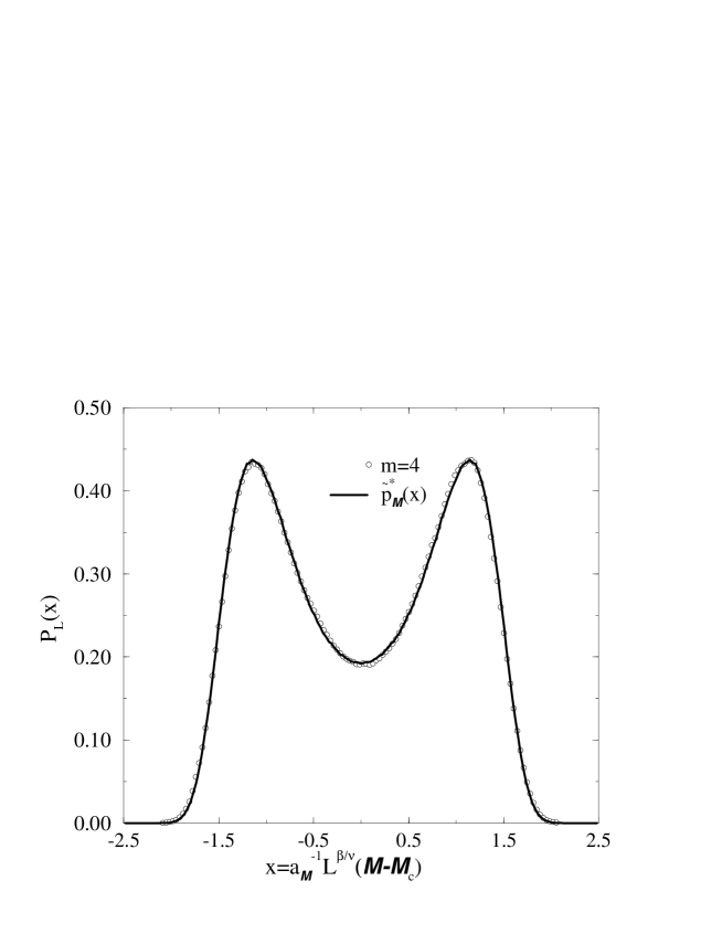
FIG. 3.: The measured form of the ordering operator distribution $p_{L}({\cal M})$ for the $m=4$ system size at the apparent critical parameters $T_{c}^{\star}=1.1853,\mu_{c}^{\star}=-2.7843$. Also shown for comparison is the universal fixed point ordering operator distribution $\tilde{p}^{\star}_{\cal M}(x)$. The data has been expressed in terms of the scaling variable $x=a_{\cal M}^{-1}L^{\beta/\nu}(\mbox{${\cal M}$}-\mbox{${\cal M}$}_{c})$, with the value of the non-universal scale factor $a_{\cal M}^{-1}$ chosen so that the distributions have unit variance. Statistical errors do not exceed the symbol sizes. From ref. [34]

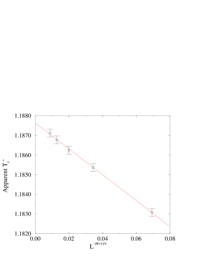
FIG. 4.: The apparent reduced critical temperature, (as defined by the matching condition described in the text), plotted as a function of $L^{-(\theta+1)/\nu}$, with $\theta=0.54$ and $\nu=0.629$ [18, 38]. The extrapolation of the least squares fit to infinite volume yields the estimate $T_{c}^{\star}=1.1876(3)$. From ref. [34]

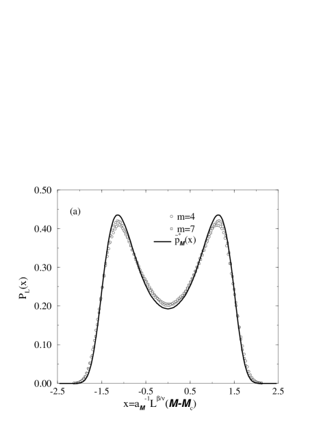
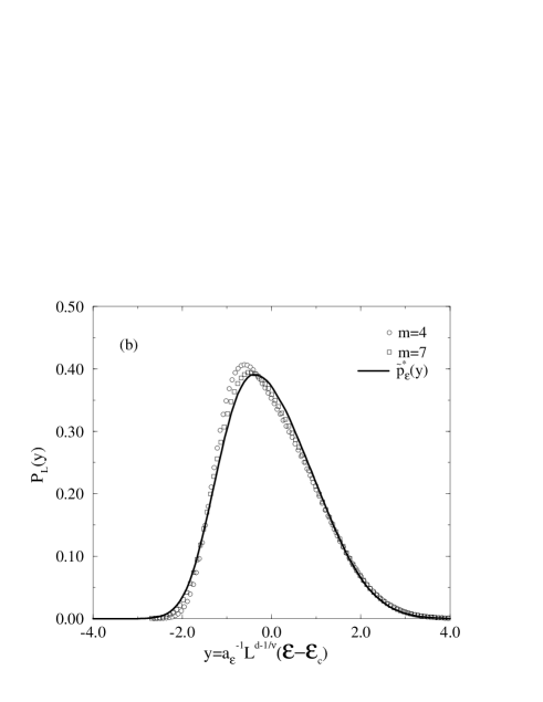
FIG. 5.: (a) The ordering operator distribution $p_{L}({\cal M})$ for the two system sizes $m=4$ and $m=7$ at the assigned critical parameters $T_{c}^{\star},\mu_{c}^{\star}$, expressed as function of the scaling variable $x=a_{\cal M}^{-1}L^{\beta/\nu}({\cal M}-{\cal M}_{c})$. Also shown (solid line) is the universal fixed point ordering operator distribution $\tilde{p}^{\star}_{\cal M}(x)$. (b) The energy operator distribution $p_{L}({\cal E})$ for the two system sizes $m=4$ and $m=7$ at $T_{c}^{\star},\mu_{c}^{\star}$ ,expressed as a function of the scaling variable $y=a_{\cal E}^{-1}L^{d-1/\nu}({\cal E}-{\cal E}_{c})$. Also shown (solid line) is the universal fixed point energy operator distribution $\tilde{p}^{\star}_{\cal E}(y)$ . In both cases the values of the non-universal scale factors $a_{\cal E}^{-1}$ or $a_{\cal M}^{-1}$ have been chosen to yield unit variance. From ref. [34]

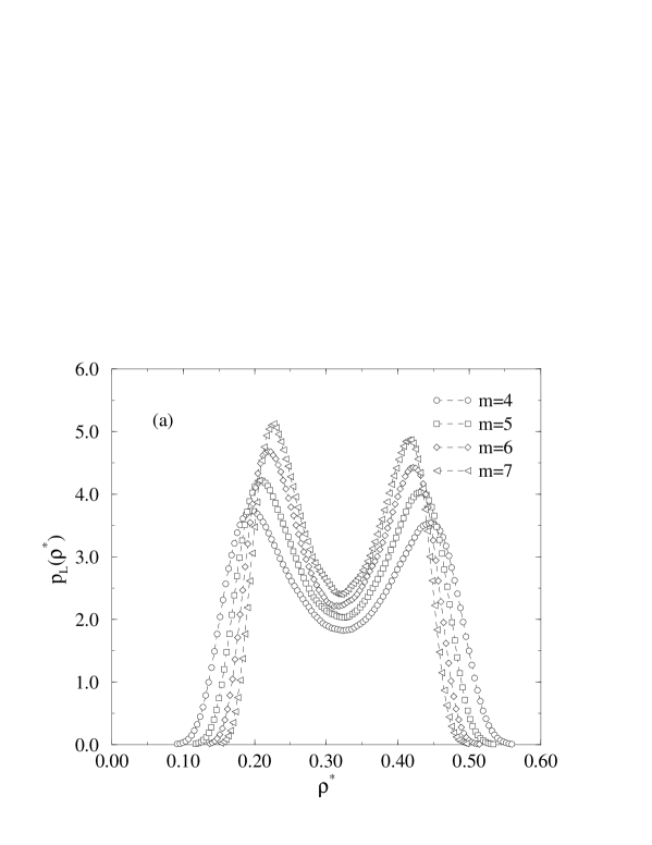
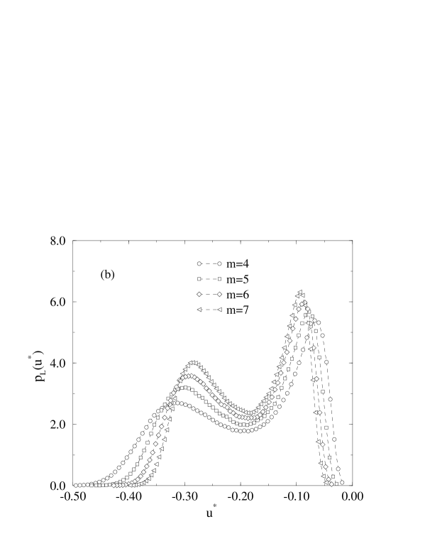
FIG. 6.: (a) The density distribution at $T_{c}^{\star},\mu_{c}^{\star}$ for the system sizes $m=4$—$7$, (b) The corresponding energy density distributions. The lines are merely guides to the eye. Statistical errors do not exceed the symbol sizes. From ref. [34]

FIG. 7.: (a) The measured average density $\langle\rho\rangle_{c}(L)$ at the designated critical point, expressed as a function of $L^{-(1-\alpha)/\nu}$. The least-squares fit yields an infinite volume estimate $\rho_{c}=0.3197(4)$. (b) The measured average energy density $\langle u\rangle_{c}(L)$ at the critical point, expressed as a function of $L^{-(1-\alpha)/\nu}$ . Extrapolation of the least-squares fit to infinite volume yields the estimate $u_{c}=-0.187(2)$. In both cases $1/\nu=1.5887$ was taken [38]. From ref. [34]

FIG. 8.: (a) Schematic phase diagram of the spin fluid in the $T$–$\rho$ plane. (b) Schematic phase diagram in the $\mu$–$T$ plane showing the directions of the relevant scaling fields $g$ and $\lambda$. From ref. [39]

FIG. 9.: The measured cumulant ratios $U_{L}$ for the 2D spin fluid model along the first order line and its analytic extension determined according to the procedure described in the text. From ref. [39]

FIG. 10.: Typical particle/spin configurations of the $L=30\sigma$ spin fluid near tricriticality. Spins values of $+1$ are denoted by filled circles, and spin values $-1$ by unfilled circles. From ref. [39]

FIG. 11.: The scaling operator distributions for the 2D spin fluid at the designated tricritical parameters for each of the three system sizes $L=18\sigma,24\sigma,30\sigma$. (a) $\tilde{p}_{L}^{\star}({\cal M})$, (b), $\tilde{p}_{L}^{\star}({\cal D})$ (c) $\tilde{p}_{L}^{\star}({\cal E})$. Also shown for comparison are the corresponding distribution measured for the tricritical $L=40$ 2D Blume-Capel model. All distributions are expressed in terms of the scaling variable $a_{i}^{-1}L^{d-y_{i}}({\cal O}-{\cal O}_{c})$ and are scaled to unit norm and variance. Statistical errors do not exceed the symbol sizes. From ref. [39]

REFERENCES

- [1] T. Andrews, Phil. Trans. R. Soc. 159 575 (1869).
- [2] H. E. Stanley Introduction to Phase transitions and critical phenomena Oxford Univ. Press, New York (1971).
- [3] J.J. Binney, N.J. Dowrick, A.J. Fisher, M.E.J. Newman The theory of critical phenomena, an introduction to the renormalization group, Clarendon Press, Oxford (1992).
- [4] P. Christe and M. Henkel, Introduction to Conformal Invariance and Its Applications to Critical Phenomena, Springer, Berlin (1993).
- [5] K. Binder in Computational Methods in Field Theory H. Gausterer, C.B. Lang (eds.) Springer-Verlag Berlin-Heidelberg 59-125 (1992).
- [6] For a review, see V. Privman (ed.) Finite size scaling and numerical simulation of statistical systems (World Scientific, Singapore) (1990).
- [7] L. P. Kadanoff in Phase transitions and critical phenomena edited by C. Domb and M. S. Green (Academic New York, 1976), Vol 5A, pp 1-34.
- [8] F.J. Wegner, Phys. Rev. B5, 4529 (1972).
- [9] J.V. Sengers and J.M.H. Levelt Sengers, Ann. Rev. Phys. Chem. 37, 189 (1986).
- [10] C.H. Back, C. Wursch, A. Vaterlaus, U. Ramsperger, U. Maier and D. Pescia, Nature 378, 597 (1995).
- [11] A.D. Bruce and N.B. Wilding, Phys. Rev. Lett. 68, 193 (1992).
- [12] N.B. Wilding and A.D. Bruce, J. Phys.: Condens. Matter 4, 3087 (1992).
- [13] K. Binder, Z. Phys. B43, 119 (1981).
- [14] A.D. Bruce, J. Phys. C 14, 3667 (1981).
- [15] J.J. Rehr and N.D. Mermin, Phys. Rev. A 8, 472 (1973).
- [16] N.B. Wilding and M. Müller, J. Chem. Phys. 102 2562 (1995).
- [17] N.B. Wilding, Z. Phys. B93, 119 (1993).
- [18] B.G. Nickel and J. J. Rehr, J. Stat. Phys. 61, 1 (1990); J.-H. Chen, M.E. Fisher and B.G. Nickel, Phys. Rev. Lett 48, 630 (1982); A. Liu and M.E. Fisher J. Stat. Phys. 58, 431 (1990).
- [19] W.F. Saam, Phys. Rev. A2, 1461 (1970).
- [20] M.A. Anisimov, Critical Phenomena in Liquids and Liquid Crystals (Gordon and Breach, Philadelphia, 1991).
- [21] M.A. Anisimov, E.E. Gorodetskii, V.D. Kulikov and J.V. Sengers, Phys. Rev. E51 1199 (1995).
- [22] M. Ley-Koo and M.S. Green, Phys. Rev. A16, 2483 (1977); M. Nakata, T. Dobashi, N. Kuwahara, M. Kaneko and B. Chu, Phys. Rev. A18 2683 (1978); Jungst S, Knuth B and Hensel F, Phys. Rev. Lett. 55 2167 (1985).
- [23] Binder K and Heermann D W 1988 Monte Carlo Simulation in Statistical Physics (Berlin: Springer)
- [24] M.P. Allen and D.J. Tildesley Computer simulation of liquids (Oxford University Press, Oxford) (1987).
- [25] N.B. Wilding in Annual Reviews of Computational Physics IV (edited by D.Stauffer) World Scientific, Singapore) (1996).
- [26] M. Rovere, D.W. Heermann and K. Binder, J. Phys.: Condens. Matter 2, 7009 (1990).
- [27] M. Rovere, P. Nielaba and K. Binder, Z. Phys. B90, 215 (1993).
- [28] N.B. Wilding and K. Binder, Physica A (in press).
- [29] E. de Miguel, E.M. del Rio and M.M. Telo da Gama, J. Chem. Phys. 103 6188 (1995).
- [30] C.-Y. Shew and A. Yethiraj, J. Chem. Phys. 104 7665 (1996).
- [31] See eg. A.Z. Panagiotopoulos, Mol. Simul. 9, 1 (1992); A.Z. Panagiotopoulos, in Observation, prediction and simulation of phase transitions in complex fluids, M. Baus, L.R. Rull and J.P. Ryckaert (eds.), NATO ASI Series C, vol 460, pp. 463-501, Kluwer Academic Publishers, Dordrecht, The Netherlands (1995).
- [32] K.K. Mon and K. Binder, J. Chem. Phys. 96, 6989 (1992).
- [33] J.R. Recht and A.Z. Panagiotopoulos, Mol. Phys. 80, 843 (1993);
- [34] N.B. Wilding, Phys. Rev. E52 602 (1995).
- [35] A.Z. Panagiotopoulos, Int. J. Thermophys. 15 1057 (1994).
- [36] A.M. Ferrenberg and R.H. Swendsen, Phys. Rev. Lett. 61 2635 (1988); A.M. Ferrenberg and R.H. Swendsen Phys. Rev. Lett. 63, 1195 (1989).
- [37] R. Hilfer and N.B. Wilding, J. Phys. A28, L281 (1995).
- [38] A.M. Ferrenberg and D.P. Landau, Phys. Rev. B44, 5081 (1991).
- [39] N.B. Wilding and P. Nielaba, Phys. Rev. E53, 926 (1996).
- [40] D. Marx, P. Nielaba and K. Binder, Phys. Rev. B47 7788 (1993).
- [41] P.C. Hemmer and D. Imbro, Phys. Rev. A16 380 (1977).
- [42] J. M. Tavares, M. M. Telo da Gama, P.I.C. Teixeira, J. J. Weis and M.J.P. Nijmeijer, Phys. Rev. E52 1915 (1995).
- [43] For a general review of tricritical phenomena see I. D. Lawrie and S. Sarbach, in Phase transitions and critical phenomena edited by C. Domb and J.L. Lebowitz (Academic London, 1984), Vol. 8.
- [44] R.B. Griffiths, Phys. Rev. B7, 545 (1973)
- [45] D. Nicolaides and A.D. Bruce, J. Phys. A 21, 233 (1988).
- [46] M.J.P. Nijmeijer and J.J. Weis, Phys. Rev. E53, 591 (1996).
- [47] M.J.P. Nijmeijer and J.J. Weis, in Annual Reviews of Computational Physics IV (edited by D.Stauffer) World Scientific, Singapore) (1996).
- [48] I. Carmesin, K. Kremer, Macromolecules 21, 2819 (1988).
- [49] A. Sariban and K. Binder, J. Chem. Phys. 86 5859 (1987).
- [50] H.-P. Deutsch and K. Binder, Macromolecules 25 6214 (1992). H.-P. Deutsch and K. Binder, J. Phys. (Paris) II 3 1049 (1993).
- [51] H.-P. Deutsch, J. Chem. Phys. 99 4825 (1993).
- [52] H.-P. Deutsch and K. Binder, J. Phys. (Paris) II 3 1049 (1993).
- [53] M. Müller and K. Binder, Computer Physics Commun.,84 173 (1994).
- [54] M. Müller and N.B. Wilding, Phys. Rev. E51 2079 (1995).
- [55] M. Müller and K. Binder, Macromolecules 28 1825 (1995).
- [56] M. Müller and M. Schick, Seattle preprint.
- [57] N.B. Wilding, M. Müller and K. Binder, J. Chem. Phys (in press).
- [58] D. Frenkel, G.C.A.M. Mooij and B. Smit, J. Phys. Condens. Matter 3, 3053 (1992).
- [59] B. Widom, Physica A194, 532 (1993).
- [60] M.E. Fisher, J. Stat. Phys. 75 1 (1994).
- [61] B.P. Lee and M.E. Fisher, Phys. Rev. Lett 76 2906 (1996).
- [62] J.M.H. Levelt-Sengers and J.A. Given, Mol. Phys. 80 899 (1993).
- [63] R.J.F. Leote de Carvalho and R. Evans, J. Phys. Condens. Matter 7, L575 (1995).
- [64] Y. Levin and M.E. Fisher, Physica A225 164 (1996).
- [65] G. Orkoulas and A.Z. Panagiotopoulos, J. Chem. Phys. 101 1452 (1994).
- [66] J.M. Caillol, D. Levesque and J.J. Wies, Preprint.
- [67] L. Vega, E. de Miguel, L. F. Rull, G. Jackson and I.A. McLure, J. Chem. Phys. 96 2296 (1992).
- [68] M.A. Anisimov, A.A. Povodyrev, V.D. Kulikov and J.V. Sengers, Phys. Rev. Lett 75 3146 (1995).
- [69] R.E Goldstein and A. Parola J. Chem. Phys. 88 7059 (1988).
- [70] S.-Y. Zinn and M.E. Fisher, Physica A226 168 (1996).
- [71] B. Berg. U. Hansmann and T. Neuhaus, Z. Phys. B90 229 (1993).
- [72] J.E. Hunter and W.P. Reinhardt, J. Chem. Phys 103 8627 (1995).