[

Density expansion for transport coefficients: Long-wavelength versus Fermi surface nonanalyticities

Abstract

The expansion of the conductivity in $2$-$d$ quantum Lorentz models in terms of the scatterer density $n$ is considered. We show that nonanalyticities in the density expansion due to scattering processes with small and large momentum transfers, respectively, have different functional forms. Some of the latter are not logarithmic, but rather of power-law nature, in sharp contrast to the $3$-$d$ case. In a $2$-$d$ model with point-like scatterers we find that the leading nonanalytic correction to the Boltzmann conductivity, apart from the frequency dependent weak-localization term, is of order $n^{3/2}$.

] It is well known from the statistical mechanics of fluids that for transport coefficients, as opposed to thermodynamic quantities, no virial or density expansion exists[2]. Let us consider a classical Lorentz gas[3], i.e. a single particle moving in a static array of scatterers with scatterer density $n$, as a simple model of a classical fluid. In such a system in three dimensions ($d=3$), the diffusion coefficient, $D$, as a function of $n$ has the form,

$$D/D_{\,\rm B}=1+D_{1}n+D_{2\ln}n^{2}\ln n+D_{2}n^{2}+o(n^{2})\ .$$ (2)

Here $D_{\,\rm B}$ denotes the Boltzmann diffusivity, $D_{1}$, $D_{\rm 2\ln}$, and $D_{2}$ are numbers, and $o(n^{2})$ denotes terms that vanish faster than $n^{2}$ for $n\rightarrow 0$. In $2$-$d$ systems, a similar nonanalyticity appears, but at one lower order in the density expansion,

$$D/D_{\,\rm B}=1+D_{1\ln}n\ln n+D_{1}n+o(n)\quad.$$ (3)

The nonanalyticities in Eqs. (Density expansion for transport coefficients: Long-wavelength versus Fermi surface nonanalyticities) are not specific to the Lorentz models, but are also present in real fluids[4]. They are a result of long range dynamical correlations in the system. If one performs a cluster expansion in a $d$-dimensional system, then ring collisions, i.e. processes where the scattered particle collides with a scatterer to which it returns after having scattered off a number of other scattering centers, lead to a logarithmic infinity in the density expansion at order $n^{d-1}$[5]. This divergence is cut off by the mean-free path. Through the density dependence of the latter, this translates into a logarithmic nonanalyticity at that order. The nature of the higher order terms is not known, but they are believed to also contain logarithmic nonanalyticities.

Since the mechanism that is believed to lead to these effects in classical systems is rather general, one would expect a similar effect to occur in the transport coefficients of quantum mechanical particles. This is indeed the case[6]. Although the leading expansion parameter is different[7], and performing the classical limit to make contact with the classical ring collisions is nontrivial[8], one obtains for a $3$-$d$ quantum system again an expansion of the form given in Eq. (2). Specifically, all of the coefficients in Eq. (2) have been calculated for a quantum Lorentz model that is a good representation of electrons injected into Helium gas[9]. It is apparent from the details of these calculations, although not from the result, that in a quantum system there are two physically distinct sources of the logarithmic nonanalyticity. These are, (1) long-wavelength contributions, i.e. those dominated by scattering processes with a momentum transfer on the order of an inverse mean-free path, and (2) Fermi surface contributions, which are dominated by momentum transfers close to $2k_{\rm F}$, with $k_{\rm F}$ being the Fermi momentum. In a dilute system, these two length scales are well separated. Again, the nature of the higher terms is not known, but inspection of some individual terms makes it appear likely that the next term in Eq. (2) is of the form $n^{3}(\ln n)^{2}$.

In this Letter we show that the fact that both of the mechanisms mentioned above yield a logarithmic nonanalyticity is characteristic of $d=3$, and that in $d=2$ some of the Fermi surface contributions lead to a power law nonanalyticity of the form $n^{3/2}$. Moreover, we find that in a $2$-$d$ quantum Lorentz model with point-like scatterers, the leading $n\ln n$ nonanalyticities cancel, so that the $n^{3/2}$ term is the leading nonanalyticity, apart from the frequency dependent weak-localization logarithm that appears in a $2$-$d$ quantum system. The density expansion for the frequency dependent conductivity, $\sigma(\omega)$, (which in a quantum system is easier to calculate than the diffusivity) in such a model thus takes the form,

$${\rm Re}\,\sigma(\omega)/\sigma_{\rm B} = 1+\frac{2}{\pi}\frac{\gamma}{2\epsilon}\ln(\omega\tau)+\sigma_{1\ln}\frac{\gamma}{2\epsilon}\ln\left(\frac{\gamma}{2\epsilon}\right)+\sigma_{1}\frac{\gamma}{2\epsilon}$$ (6)

$$+\ \sigma_{3/2}\left(\frac{\gamma}{2\epsilon}\right)^{3/2}+o\left(\frac{\gamma}{2\epsilon}\right)^{3/2}\quad,$$

where we have left out contributions that vanish as $\omega\rightarrow 0$. Here $\sigma_{\rm B}{=}e^{2}\epsilon\tau/(2\pi m)$ denotes the Boltzmann conductivity, $\tau$ is the scattering mean-free time, $m$ is the electron mass, $\epsilon=k_{\rm F}^{2}$, and $\gamma=m/\tau=n\sigma_{T}k_{F}$, with $\sigma_{T}$ the total s-wave cross-section, is a convenient expansion parameter that is proportional to the impurity density. The $\ln(\omega\tau)$ term is the so-called weak-localization correction (see below), whose prefactor has been known for some time. For the remaining coefficients in Eq. (6) we find,

$$\sigma_{1\ln}=0\ ,\ \sigma_{1}=\frac{2}{\pi}\,(1-\ln 2)\ ,\ \sigma_{3/2}=3/2\sqrt{2}\ .$$ (7)

Equations (Density expansion for transport coefficients: Long-wavelength versus Fermi surface nonanalyticities) constitute our result. Before we sketch its derivation, let us explain the physical origin of the $\gamma^{3/2}$ term in Eq. (6). In a degenerate system of noninteracting fermions, the Pauli principle restricts the phase space that is available in scattering processes. These restrictions lead, e.g., to the well-known nonanalyticity of the Lindhard function at a momentum $q=2k_{\rm F}$. The nature of this nonanalyticity is dimensionality dependent; it is logarithmic in $d=3$, and a square root in $d=2$. The same phase space restrictions lead to related nonanalyticities in the scattering cross section, and hence in the transport coefficients. This is precisely what we find. The effect we predict is thus a consequence of the sharpness of the Fermi surface. It is related to other phenomena resulting from the degenerate nature of a Fermi gas at $T=0$, like, e.g., the Friedel oscillations, and the Kohn anomaly.

We now outline the derivation of our results. Let us consider the standard Edwards model of noninteracting electrons in $d=2$ in an environment of static, spatially random scatterers. The model Hamiltonian reads,

$$H=\sum_{\bf k}\,(\epsilon_{{\bf k}}-\mu)\ a^{{\dagger}}_{\bf k}a_{\bf k}+\sum_{{\bf k},{\bf q}}\,{\hbox{V({\bf q})}}\ a^{{\dagger}}_{{\bf k}+{\bf q}/2}\,a_{{\bf k}-{\bf q}/2}\quad,$$ (8)

where $a^{{\dagger}}_{\bf k}$ and $a_{\bf k}$ denote the creation and annihilation operators, respectively, for electrons with wave vector ${\bf k}$, $\mu$ is the chemical potential, $V({\bf q})$ is the Fourier transform of the electron-impurity scattering potential, and $\epsilon_{{\bf k}}={\bf k}^{2}/2m$. Throughout this paper we use units such that $\hbar=1$. Also, we will be working at zero temperature, so we put $\mu=\epsilon_{\rm F}=k_{\rm F}^{2}/2m$. Since we are dealing with noninteracting electrons, spin just leads to trivial factors of two and can be omitted. Standard diagrammatic perturbation theory[10] is formulated in terms of retarded (R) and advanced (A) zero temperature Green’s functions,

$${\cal G}^{R,A}_{{\bf k},{\bf p}}(\omega)=\left\langle{\bf k}\left|\frac{1}{\omega-H\pm i0}\right|{\bf p}\right\rangle$$ (10)

and their impurity averaged counterparts $\{{\cal G}^{R,A}_{\bf k,p}(\omega)\}_{\rm dis}$, where $\{\ldots\}_{\rm dis}$ denotes the average over the quenched disorder. It is most convenient to keep only the lowest order contribution to the self energy in the averaged Green’s function, so we will use as the building blocks of our perturbation theory the following approximation to $\{{\cal G}^{R,A}_{\bf k,p}(\omega)\}_{\rm dis}$,

$$G^{R,A}_{\bf k}=\frac{1}{\omega-(\epsilon_{\bf k}-\epsilon_{\rm F})\pm i\gamma/2m}\quad.$$ (11)

In writing Eq. (11), we have specialized to the case of pure s-wave scattering, or a point-like impurity potential, i.e. we have put $V({\bf q})\equiv U=\gamma/4\pi^{2}m^{2}$[11].

The transport coefficient of interest to us, viz. the dynamical conductivity $\sigma(\omega)$, can be expressed in terms of the Green’s functions by means of the Kubo-Greenwood formula,

$${\rm Re}\,\sigma(\omega) = \frac{e^{2}}{\pi m^{2}}\,{\rm Re}\,\sum_{\bf k,p}\ k_{z}\ \left\{{\cal G}^{R}_{\bf k,p}(\omega)\,{\cal G}^{A}_{\bf p,k}(\omega=0)\right.$$ (13)

$$\left.-\,{\cal G}^{R}_{\bf k,p}(\omega)\,{\cal G}^{R}_{\bf p,k}(\omega=0)\right\}_{\rm dis}\ p_{z}\quad,$$

This expression can be used to systematically expand $\sigma$ in powers of $\gamma$. Such an expansion has been set up in Ref. [7], and in Ref. [9] all diagrams were identified that contribute up to and including order $\gamma^{2}$ in $d=3$. The classification of the diagrams with respect to the order in $\gamma$ they contribute to does not carry over to other values of $d$, but it turns out that the diagrams that contribute to the terms shown in Eq. (6) form a subset of those considered in Ref. [9]. They are shown in Figs. 1 - 3.

FIG. 1.: Simple diagrams that contribute to the terms shown in Eq. (6). For each of the diagrams (f) and (j) there is one equivalent symmetric diagram (not shown) that also contributes, and the complex conjugates of diagrams (b) - (f) and (h) - (j) contribute as well. The ‘triangulated’ line in diagram (b) denotes a Green’s function, Eq. (11), with its value at $\gamma=0$ subtracted to avoid double counting. Diagram (a) yields $\sigma_{B}+O(\gamma^{2})$ and serves to normalize all other contributions. Diagrams (e) - (g) contribute to the $\gamma^{3/2}$ term.

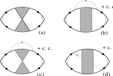
FIG. 2.: Infinite resummations that contribute to the terms shown in Eq. (6). The complex conjugates of diagrams (b) - (d) contribute as well.

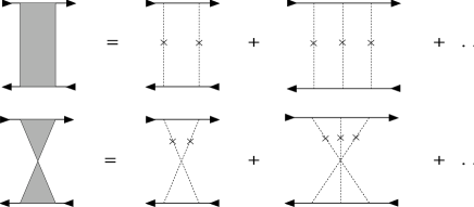
FIG. 3.: Definition of the vertices in Fig. 2.

All of these diagrams can be expressed in terms of integrals over combinations of two functions, $J^{++}$ and $J^{+-}$, that are convolutions of $G^{R}$ and $G^{A}$. At zero frequency they are defined as,

$$J^{+\nu}(q)=\int d{\bf k}\ \frac{1}{\epsilon-k^{2}+i\gamma}\,\frac{1}{\epsilon-({\bf k}-{\bf q})^{2}+i\nu\gamma}\quad,$$ (15)

with $\nu=\pm$. Doing the integrals yields, in $d=2$,

$$J^{++}(q)=\frac{2\pi}{qw_{++}}\,\left[\ln(w_{++}+q)-\ln(w_{++}-q)\right]\quad,$$ (16)

$$J^{+-}(q) = \frac{-2i\pi}{w_{+-}}\,\left[\ln\left(\frac{w_{+-}+2\gamma-iq^{2}}{w_{+-}+2\gamma+iq^{2}}\right)\right.$$ (18)

$$+\left.\frac{1}{2}\ln\left(\frac{\epsilon-i\gamma}{\epsilon+i\gamma}\right)+i\pi\right]\quad,$$

where,

$$w_{++}=\sqrt{w(q)-4i\gamma}\quad,\quad w_{+-}=\sqrt{-q^{2}w(q)+4\gamma^{2}}\quad,$$ (19)

with $w(q)=q^{2}-4\epsilon$.

The only diagrams that contribute to the $\gamma^{3/2}$ term in Eq. (6) are (e), (f), and (g) in Fig. 1. In order to demonstrate how the nonanalyticity arises, let us consider diagram (g) as an example. After simple manipulations, its contribution to the conductivity can be written,

$$\frac{\sigma^{\rm(1g)}}{\sigma_{B}}=\left(\frac{\gamma}{2\epsilon}\right)^{2}\,\frac{4\epsilon^{2}}{\pi^{8}}\int d{\bf q}\ {\rm Re}\,J^{++}(q)\,{\rm Re}[J^{++}(q)]^{2}\quad.$$ (20)

Here we have put $\omega=0$, and have kept only the leading contribution for $\gamma\rightarrow 0$. It is now easy to see how the nonanalyticity arises. Equation (16) shows that, in the limit $\gamma\rightarrow 0$, $J^{++}$ contains a singularity of the form $(q-2k_{\rm F})^{-1/2}$. A $q$-integration over $(J^{++})^{3}$ thus leads to a $\gamma^{-1/2}$ term. Since $(J^{++})^{3}$ first appears in the integrands at order $\gamma^{2}$, the leading singularity produced by this mechanism is of the form $\gamma^{3/2}$. Asymptotic analysis yields the prefactor of the nonanalyticity, which gives a contribution to the number $\sigma_{3/2}$ in Eq. (6) as stated in Table I. Similarly, an integral over $(J^{++})^{2}$ produces an $\ln\gamma$, and this mechanism contributes to the prefactor $\sigma_{1\ln}$ in Eq. (6). Another contribution to $\sigma_{1\ln}$ comes from the ‘long-wavelength’ terms, which manifest themselves as integrals $\int d{\bf q}\ [J^{+-}(q)]^{2}$. Such integrals arise from Fig. 1 (d) (in (c) they cancel), and Fig. 2 (a). The fact that in $d=2$ two powers of $J^{+-}$ are sufficient to produce a logarithm accounts for the fact that this nonanalyticity appears already at linear order in $\gamma$. Finally, some of the diagrams discussed so far, and all of the remaining ones, contribute to the analytic term at order $\gamma$. The various contributions are listed in Table I.

TABLE I.: Contributions of diagrams as shown in Figs. 1 and 2 to the coefficients in Eq. (6). No entry means that the diagram does not contribute for structural reasons, while a zero indicates no contribution due to cancellations.

diagram	$\sigma_{1\ln}$	$\sigma_{1}$	$\sigma_{3/2}$
1 (b)		$2/\pi$
1 (c)		$0$
1 (d)	$-2/\pi$	$-(8/\pi)\ln 2$
1 (e)			$-\sqrt{2}/2$
1 (f)			$\sqrt{2}$
1 (g)			$\sqrt{2}/4$
1 (h)			$0$
1 (i)			$0$
1 (j)			$0$
2 (a)	$2/\pi$	$(4/\pi)\ln 2$
2 (b)+(c)+(d)		$(2/\pi)\ln 2$

The infinite resummation denoted by diagram (a) in Fig. 2 plays a special role in our perturbation theory, and deserves some discussion. This ‘crossed ladder’ resummation is the only diagram where the zero-frequency limit needs to be handled with some care, since it is related to the so-called weak-localization anomaly, i.e. the fact that the conductivity of disordered noninteracting electrons in $d=2$ contains a $\ln\omega\tau$ in perturbation theory, and that the true zero-frequency value of $\sigma$ is zero[12]. Taken at face value, the diagram is finite at $\omega=0$, since the resummation leads to a structure $1/(1-\gamma J^{+-}(q)/\pi^{2})$. Expanding $J^{+-}$ in powers of $\gamma$ leads to a diffusion pole, i.e. a $1/q^{2}$ singularity, at lowest order, but the subleading contribution of $O(1)$ to $J^{+-}(q=0)$ seems to protect the singularity. This is misleading, however, since it is well known that the ‘crossed ladder’ is an approximation to an exact vertex part $\Lambda(q,\omega)$ that has an exact diffusion pole, $\Lambda(q,\omega)\sim 1/(-i\omega+q^{2}/D)$, with $D$ the diffusion coefficient[13]. Indeed one can show that there exist classes of diagrams that cancel the mass in the simple crossed ladder, order by order in perturbation theory[14]. Although formally of higher order in $\gamma$, these contributions lead to the logarithmic singularity stemming from $\Lambda$ being protected only by a finite frequency, and not by $\gamma$. On a more formal level, strict perturbation theory in powers of $\gamma$ violates a Ward identity that reflects particle number conservation in the presence of time reversal invariance. By choosing a self energy that is related to the crossed ladder vertex correction by means of this Ward identity, one can construct a conserving approximation for $\Lambda$ which has the diffusion pole built in. Replacing the small-$q$ part of the crossed ladder by the appropriate exact diffusion pole then leads to the term $\ln\omega\tau$ with a prefactor as first reported by Gorkov et al., Ref. [12], and made rigorous by Kirkpatrick and Dorfman[7], and shown in Eq. (6). Apart from this, the first term in the infinite crossed ladder resummation also contributes to the coefficients $\sigma_{1}$ and $\sigma_{1\ln}$, see Table I.

We have ascertained that no other diagrams contribute to the terms we are considering. For simple diagrams, it is easy to show, by a combination of the diagram rules with power counting, that diagrams with more than three impurity lines cannot contribute. For the infinite resummations, the same type of argument shows that dressing the diagrams shown in Fig. 2 by additional impurity lines leads to terms that vanish faster than $\gamma^{3/2}$. Finally, arguments analogous to those employed before in $d=3$[9] show that one need not consider diagrams with more than one ladder or crossed ladder resummation.

We also mention that the temperature dependent conductivity is easily obtained from our $T=0$ result by a convolution with the derivative of a Fermi function[15, 9]. At low temperatures, the $\gamma^{3/2}$ anomaly then gets translated into a $T^{3/2}$ dependence at fixed scatterer density. After subtracting out the weak-localization term, this should be observable, at least in principle, in experiments of the type reported by Adams[16].

We gratefully acknowledge helpful discussions with T.R. Kirkpatrick. This work was supported by the NSF under grant number DMR-95-10185.

REFERENCES

- [1] Present address: Victron Inc., 2530 Zanker Rd., San Jose, CA 95131.
- [2] See, e.g., R. Peierls, Surprises in Theoretical Physics, Princeton University (Princeton 1979), ch. 5.1, for a nontechnical description; or J. R. Dorfman, T. R. Kirkpatrick, and J. V. Sengers, Ann. Rev. Phys. Chem. 45, 213 (1994), for a recent technical review.
- [3] For a discussion of Lorentz models, see, E. H. Hauge, in Transport Phenomena, Lecture Notes in Physics No. 31, edited by G. Kirczenow and J. Marro, Springer (New York 1974), p.337.
- [4] In a real classical fluid, the static diffusivity does not exist due to long-time tail effects, so one also needs to consider the frequency dependence. A similar effect occurs in the quantum Lorentz model to be studied below.
- [5] The role of ring collisions in this context has sometimes be disputed. See, R.F. Fox, Phys. Rev. A 27, 3216 (1983).
- [6] J. S. Langer and T. Neal, Phys. Rev. Lett. 16, 984 (1966); J. Weinstock, ibid. 17, 130 (1966).
- [7] T. R. Kirkpatrick and J. R. Dorfman, Phys. Rev. A 28, 1022 (1983). See also T. R. Kirkpatrick and D. Belitz, Phys. Rev. B 34, 2168 (1986).
- [8] P. Resibois and M. G. Velarde, Physica 51, 541 (1971).
- [9] K. I. Wysokiński, Wansoo Park, D. Belitz, T.R. Kirkpatrick, Phys. Rev. E 52, 612 (1995).
- [10] See, e.g., G. D. Mahan Many–Particle Physics (Plenum Press, New York and London, 1981), ch. 7.
- [11] In , pure s-wave scattering is an excellent approximation to the scattering processes in certain systems[9]. In this is not the case, and a more realistic description of the scattering process would lead to quantitative changes of our coefficients. In particular, may hold only for point-like scatterers. However, the existence of the term is independent of this approximation.
- [12] E. Abrahams, P. W. Anderson, D. C. Licciardello, and T. V. Ramakrishnan, Phys. Rev. Lett. 42, 673 (1979) first showed that in . The connection with the crossed ladder was pointed out by L. P. Gor’kov, A. I. Larkin, D. E. Khmel’nitskii, Pis’ma Zh. Eksp. Teor. Fiz. 30, 248 (1979) [JETP Lett. 30, 228 (1979)]. For a review of this subject, see, P. A. Lee and T. V. Ramakrishnan, Rev. Mod. Phys. 57, 287 (1985). The importance of considering both the frequency and the density dependence of has been stressed by D. Belitz and T. R. Kirkpatrick, Rev. Mod. Phys. 66, 261 (1994).
- [13] D. Vollhardt and P. Wölfle, Phys. Rev. B 22, 4666 (1980).
- [14] We thank T. R. Kirkpatrick for a discussion of this point.
- [15] D. A. Greenwood, Proc. Phys. Soc. 71, 585 (1958).
- [16] P. W. Adams, Phys. Rev. Lett. 65, 333 (1990).