[

Low temperature spin diffusion in the
one-dimensional quantum $O(3)$ nonlinear $\sigma$-model

Abstract

An effective, low temperature, classical model for spin transport in the one-dimensional, gapped, quantum $O(3)$ non-linear $\sigma$-model is developed. Its correlators are obtained by a mapping to a model solved earlier by Jepsen. We obtain universal functions for the ballistic-to-diffusive crossover and the value of the spin diffusion constant, and these are claimed to be exact at low temperatures. Implications for experiments on one-dimensional insulators with a spin gap are noted.

]

Over the past decade, a large number of one-dimensional, insulating, Heisenberg antiferromagnets with a zero temperature ($T$) spin gap have been studied: these include integer spin chains [1, 2] and half-integer spin-ladder systems [3]. In the large spin $S$ limit, the low energy properties of these compounds are described [4] by the one-dimensional quantum $O(3)$ non-linear $\sigma$-model (without any topological term), and there is evidence [5] that the mapping to this continuum model is quantitatively accurate even for the $S=1$ spin chain. Theoretically, much is known about the quantum field theory of the $\sigma$-model [6, 7, 8], and this information has been valuable in understanding the properties of the spin chains. The low energy spectrum of the $\sigma$-model consists of a triplet of massive particles, and their ballistic propagation describes many exactly known dynamic correlations at $T=0$. For $T>0$ however, exact results have so far been limited to static, thermodynamic observables [9].

In this paper, we obtain dynamic, non-zero $T$ correlators using a semiclassical method [11]: we claim that all of our results are asymptotically exact at low $T$, but this has not been rigorously established. We present universal functions which describe the crossover from ballistic spin transport at short scales, to diffusive behavior at the longest scales; as a bi-product, these functions yield the exact value of the spin diffusion constant. The nature of spin transport for any small $T>0$ is therefore qualitatively different from that at $T=0$.

The imaginary time ($\tau$) action of the $\sigma$-model is

$${\cal A}=\frac{c}{2g}\int_{0}^{1/T}d\tau dx\left[(\partial_{x}n_{\alpha})^{2}+\frac{1}{c^{2}}(\partial_{\tau}n_{\alpha}-i\epsilon_{\alpha\beta\gamma}H_{\beta}n_{\gamma})^{2}\right]$$

where $x$ is the spatial co-ordinate, $\alpha,\beta,\gamma=1,2,3$ are $O(3)$ vector indices over which there is an implied summation, $\epsilon_{\alpha\beta\gamma}$ is the totally antisymmetric tensor, $c$ is a velocity, $H_{\alpha}$ is an external magnetic field, and the partition function is obtained by integrating over the unit vector vield $n_{\alpha}(x,\tau)$, with $n_{\alpha}^{2}(x,\tau)=1$. We use units in which $\hbar=k_{B}=1$ and have absorbed a factor of the electronic magnetic moment, $g_{e}\mu_{B}$, into the definition of the field $H$. The dimensionless coupling constant $g$ is determined by the underlying lattice antiferromagnet at the momentum scale $\Lambda\sim\mbox{inverse lattice spacing}$ to be $g\sim 1/S$. We shall only be interested in the physics at length scales $\gg\Lambda^{-1}$ and time scales $\gg(c\Lambda)^{-1}$; this physics is universally characterized by the dimensionful parameters $c$, $H$, $T$, and $\Delta$, the energy gap at $T=H=0$. The magnitude of $\Delta$ is determined by non-universal lattice scale physics ($\Delta\sim c\Lambda e^{-2\pi/g}$ for small $g$). However, the long distance physics depends on these lattice scale effects only through the value of $\Delta$, and has no direct dependence on $g$ or $\Lambda$.

We shall study correlators of the magnetization density, $M_{\alpha}(x,\tau)=\delta{\cal A}/\delta H_{\alpha}(x,\tau)$. In the Hamiltonian formalism, this magnetization is measured by the operator $\hat{M}_{\alpha}(x)$, and we shall focus on the real time, finite $T$ correlation function

$$C_{\alpha\beta}(x,t)=\left\langle e^{i\hat{\cal H}t}\hat{M}_{\alpha}(x)e^{-i\hat{\cal H}t}\hat{M}_{\beta}(0)\right\rangle-\left\langle\hat{M}_{\alpha}\right\rangle\left\langle\hat{M}_{\beta}\right\rangle$$

where $\hat{\cal H}$ is the Hamiltonian corresponding to the action ${\cal A}$, and the expectation values are with respect to the density matrix $e^{-\hat{\cal H}/T}/\mbox{Tr}e^{-\hat{\cal H}/T}$. The dimensions of $M$ are inverse length, and because $M$ is a conserved density, it does not acquire any anomalous dimension (i.e. no prefactors of powers of $\Lambda$ or $\ln\Lambda$ are required to obtain a finite $\Lambda\rightarrow\infty$ limit), and its correlators are simply universal functions of combinations of $x$, $t$, $c$, $T$, $H$ and $\Delta$ which are consistent with naive dimensional analysis in lengths and times [12]. For $H\ll\Delta$ (which we assume throughout), these correlators describe the crossover between two distinct limiting physical regimes: (i) $T\ll\Delta$, the ‘quantum-disordered’ regime, where strong quantum fluctuations create a paramagnetic ground state, and the excitations consist of a triplet of particles with energy $(\Delta^{2}+c^{2}p^{2})^{1/2}$ at momentum $p$, and (ii) $\Delta\ll T\ll c\Lambda$, the high $T$ regime of the continuum theory, where quantum fluctuations are marginally subdominant [13] (by a factor of $1/\ln(T/\Delta)$), and the excitations are a doublet of spin-waves about a locally ordered state; however thermal fluctuations of classically interacting spin-waves lead again to a paramagnetic state. The crossover between these regimes has been described for the static, uniform, spin susceptibility, $\chi$, of the $O(N=\infty)$ model [14].

In this paper, we shall obtain the space-time dependent $C(x,t)$ of the $O(3)$ model in the low $T$ region $T\ll\Delta$. The ratio $H/T$ is however allowed to be arbitrary. A recent paper [10] computed $C(0,t)$ by arguing that the triplet of particles could be considered free at low enough $T$. Actually, such an approach is valid only for $|t|$ shorter than the mean collision time $\sim e^{\Delta/T}/T$ (see below), and it is essential to include particle collisions at longer $|t|$ to obtain the crossover to diffusive behavior. Our semiclassical approach does this, and is valid for all $|t|\gg 1/T$.

There are two key observations that allow our exact computation for $T\ll\Delta$. The first [11] is that as there is an excitation gap, the density of particles $\sim e^{-\Delta/T}$, and their mean spacing is much larger than their thermal de-Broglie wavelength $\sim c/(\Delta T)^{-1/2}$; as a result the particles can be treated semiclassically. In particular, taking the field $H$ pointing along the 3 direction, the density of a particle with longitudinal spin $m$ ($m=-1,0,1$) is

$$\rho_{m}=\int\frac{dp}{2\pi}e^{-(\Delta-mH+c^{2}p^{2}/2\Delta)/T}=\sqrt{\frac{T\Delta}{2\pi c^{2}}}e^{-(\Delta-mH)/T},$$

and therefore the total density $\rho=\rho_{-1}+\rho_{0}+\rho_{1}$, and the magnetization $\langle M_{\alpha}\rangle=(\rho_{1}-\rho_{-1})\delta_{\alpha 3}$. The second observations is that collisions between these particles are described by their known two-particle $S$-matrix [7], and only a simple limit of this $S$-matrix is needed in the low $T$ limit. The r.m.s. velocity of a thermally excited particle $v_{T}=c(T/\Delta)^{1/2}$, and hence its ‘rapidity’ $\sim v_{T}/c\ll 1$. In this limit, the $S$-matrix for the process in Fig 1 is [7]

$${\cal S}^{m_{1}m_{2}}_{m^{\prime}_{1},m^{\prime}_{2}}=(-1)\delta_{m_{1}m^{\prime}_{2}}\delta_{m_{2}m^{\prime}_{1}}.$$ (1)

In other words, the excitations behave like impenetrable particles which preserve their spin in a collision.

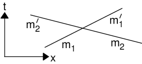
FIG. 1.: Two particle collision described by the $S$-matrix (1). The momenta before and after the collision are the same, so the figure also represents the spacetime trajectories of the particles.

Energy and momentum conservation in $d=1$ require that these particles simply exchange momenta across a collision (Fig 1). The $(-1)$ factor in (1) can be interpreted as the phase-shift of repulsive scattering between slowly moving bosons in $d=1$. Indeed, it appears that the simple form of (1) is due to the slow motion of the particles, and is not a special feature of relativistic continuum theory: we conjecture that (1) also holds for lattice Heisenberg spin chains in the limit of vanishing velocities.

We now evaluate $C(x,t)$ along the lines of a recent computation for the Ising model [11]. We represent $C(x,t)$ as a ‘double time’ path integral, with the $e^{-i\hat{\cal H}t}$ factor generating trajectories that move forward in time, and the $e^{i\hat{\cal H}t}$ producing trajectories that move backward in time. In the classical limit, stationary phase is achieved when the trajectories are time-reversed pairs of classical paths (Fig 2).

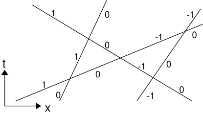
FIG. 2.: A typical set of particle trajectories contributing to $C(x,t)$. Each trajectory represents paths moving both forward and backward in time. The particle co-ordinates are $x_{k}(t)$, with the labels $k$ chosen so that $x_{k}(t)\leq x_{l}(t)$ for all $t$ and $k<\ell$. Shown on the trajectories are the values of the particle spins $m_{k}$ which are independent of $t$ in the low $T$ limit.

Each trajectory has a spin label which obeys (1) at each collision; however as each collision contributes both to the forward and backward trajectories, the net numerical factor is simply $+1$. All of this implies [11] that the lines in Fig 2 are independently distributed uniformly in space, and with an inverse slope determined by the velocity $v$ which is distributed according to the classical Boltzmann probability density ${\cal P}(v)\propto e^{-\Delta v^{2}/2c^{2}T}$. The spin, $m$, is assigned randomly at some initial time with probability $f_{m}\equiv\rho_{m}/\rho=e^{mH/T}/(1+2\cosh(H/T))$, but then evolves in time as discussed above (Fig 2).

We label the particles consecutively from left to right by an integer $k$ (see the caption of Fig 2); then their spins $m_{k}$ are independent of $t$, and we denote their trajectories $x_{k}(t)$. The longitudinal correlation $C_{33}$ is given by the correlators of the classical observable

$$M_{3}(x,t)=\sum_{k}m_{k}\delta(x-x_{k}(t))$$ (2)

in the classical ensemble defined above. Now because the spin and spatial co-ordinates are independently distributed, the correlators of $m_{k}$ and $x_{k}$ factorize. The correlators of the $m_{k}$ are easily evaluated:

$$\langle m_{k}m_{\ell}\rangle=A_{1}+A_{2}\delta_{k\ell}$$ (3)

where $A_{1}\equiv(f_{1}-f_{-1})^{2}$ and $A_{2}\equiv f_{1}+f_{-1}-(f_{1}-f_{-1})^{2}$ are simple, dimensionless, known functions of $H/T$ only. Using (3) we have

$$C_{33}(x-x^{\prime},t-t^{\prime})=A_{1}\left(\left\langle\rho(x,t)\rho(x^{\prime},t^{\prime})\right\rangle-\rho^{2}\right)$$ (4)

$$~{}~{}~{}~{}~{}~{}~{}~{}+A_{2}\sum_{k}\left\langle\delta(x-x_{k}(t))\delta(x^{\prime}-x_{k}(t^{\prime}))\right\rangle$$ (5)

where $\rho(x,t)=\sum_{k}\delta(x-x_{k}(t))$ is the spacetime dependent total density, all averages are now with respect to the classical ensemble, and $\langle\rho(x,t)\rangle=\rho$. The two-point correlators of $\rho(x,t)$ are also easy to evaluate: if the spin labels are neglected, the trajectories in Fig 2 are straight lines, and the density correlators are simply those of a classical ideal gas of point particles. The second correlator in (5), multiplying $A_{2}$, is more difficult: it involves the self correlation a given particle $k$, which follows a complicated trajectory in the way we have labeled the particles (e.g. the trajectory of the $-1$ in Fig 2). Fortunately, precisely this correlator was considered three decades ago by Jepsen [15] and a little later by others [16]; they showed that, at sufficiently long times, each such particle executes free Brownian motion. Inserting their results into (5), we obtained the final results presented below after some straightforward simplifications.

An important property of the results is that they can written in a ‘reduced’ scaling form [12] determined by the classical dynamics. From the many independent parameters $c$, $\Delta$, $T$, and $H$, only a single length ($L_{x}$) and a single time ($L_{t}$) scale controls their spacetime dependence. These scales can be chosen to be

$$L_{x}=\frac{1}{\rho}~{}~{}~{}~{}~{}L_{t}=\frac{1}{\rho}\left(\frac{\Delta}{2c^{2}T}\right)^{1/2}.$$ (6)

Notice $L_{x}\sim ce^{\Delta/T}/\sqrt{\Delta T}$ is the mean spacing between the particles , and $L_{t}\sim e^{\Delta/T}/T$ is a typical time between particle collisions as $v_{T}=L_{x}/L_{t}\sqrt{2}$. Our final result is

$$C_{33}(x,t)=\rho^{2}\left[A_{1}F_{1}\left(\frac{|x|}{L_{x}},\frac{|t|}{L_{t}}\right)+A_{2}F_{2}\left(\frac{|x|}{L_{x}},\frac{|t|}{L_{t}}\right)\right]$$ (7)

where $\rho^{2}F_{1}$ is the connected density correlator of a classical ideal gas in $d=1$,

$$F_{1}(\bar{x},\bar{t})=e^{-\bar{x}^{2}/\bar{t}^{2}}/\bar{t}\sqrt{\pi},$$ (8)

and $\rho^{2}F_{2}$ is the correlator of a given labeled particle [15, 16],

$$F_{2}(\bar{x},\bar{t})=\Biggl{[}\left(2G_{1}(u)G_{1}(-u)+F_{1}(\bar{x},\bar{t})\right)$$ (9)

$$~{}~{}~{}~{}~{}~{}~{}~{}~{}~{}~{}~{}~{}~{}~{}~{}\times I_{0}\left(2\bar{t}\sqrt{G_{2}(u)G_{2}(-u)}\right)$$ (10)

$$~{}~{}~{}~{}~{}~{}~{}~{}~{}~{}~{}~{}~{}~{}~{}~{}~{}+\frac{G_{1}^{2}(u)G_{2}(-u)+G_{1}^{2}(-u)G_{2}(u)}{\sqrt{G_{2}(u)G_{2}(-u)}}$$ (11)

$$~{}~{}~{}~{}~{}~{}~{}~{}~{}~{}~{}~{}\times I_{1}\left(2\bar{t}\sqrt{G_{2}(u)G_{2}(-u)}\right)\Biggr{]}e^{-(G_{2}(u)+G_{2}(-u))\bar{t}}$$ (12)

with $u\equiv\bar{x}/\bar{t}$, $G_{1}(u)=\mbox{erfc}(u)/2$, and $G_{2}(u)=e^{-u^{2}}/(2\sqrt{\pi})-uG_{1}(u)$. These expressions satisfy $\int_{0}^{\infty}d\bar{x}F_{1,2}(\bar{x},\bar{t})=1/2$, which ensures the conservation of the total magnetization density with time. For $|\bar{t}|\ll|\bar{x}|\ll 1$, the function $F_{2}$ has the ballistic form $F_{2}(\bar{x},\bar{t})\approx F_{1}(\bar{x},\bar{t})$, while for $|\bar{t}|\gg 1,|x|$ it crosses over to the diffusive form

$$F_{2}(\bar{x},\bar{t})\approx\frac{e^{-\sqrt{\pi}\bar{x}^{2}/2\bar{t}}}{(4\pi\bar{t}^{2})^{1/4}}~{}~{}~{}~{}\mbox{for large $\bar{t}$.}$$ (13)

In the original dimensionful units, (6) and (13) imply a spin diffusion constant, $D_{s}$, given exactly by

$$D_{s}=\frac{c^{2}e^{\Delta/T}}{\Delta(1+2\cosh(H/T))}.$$ (14)

Let us now consider correlations of the transverse magnetization. It is convenient to work with the circularly polarized components of the magnetization $M_{\pm}=M_{1}\pm iM_{2}$. The analog of (2) is now $M_{\pm}=\sum_{k}S_{\pm k}\delta(x-x_{k}(t))$, where $S_{+k}$ ($S_{-k}$) are the spin raising (lowering) operators of particle $k$. In the double time path integral for $C_{-+}(x,t)$ the spin on some particle $k$ is raised at time $t=0$ in the forward trajectory; at time $t$ the lowering operator must act on the same particle or otherwise the trace over the classical trajectories vanishes. Notice also that there is no raising or lowering of spins in the backward trajectory. As a result, the path integral picks up a factor of $e^{iHt}$ from the additional Berry phase accumulated during the time the spin is raised during the forward trajectory, which is not compensated by the backward trajectory. This phase is multiplied by the self-correlation of the particle whose spin was raised, a quantity we have obtained above. Similar considerations apply to $C_{+-}$ and the final results are

$$C_{\mp\pm}(x,t)=2\rho^{2}e^{\pm iHt}A_{\mp}F_{2}\left(\frac{|x|}{L_{x}},\frac{|t|}{L_{t}}\right)$$ (15)

where $A_{\mp}\equiv f_{0}+f_{\mp 1}$.

Next, we compute the local dynamic structure factor $S_{\alpha\beta}(\omega)=\int_{-\infty}^{\infty}dte^{-i\omega t}C_{\alpha\beta}(0,t)$. A subtlety arises in computing this Fourier transform. Notice that at short $|t|\ll L_{t}$, we have the ballistic behavior $C(0,t)\sim 1/|t|$, and so the $t$ integral is logarithmically divergent. Our semiclassical results are valid only for $|t|\gg 1/T$, and so we should cut-off the integral at small $t$, leading to a contribution $\sim\ln(bT/\omega)$ where $b$ is a numerical factor of order unity. In fact, it is possible to determine $b$ precisely: at these short times the earlier free quantum particle approach [10] is valid, and we determine $b$ by matching the logarithm to their results. In physical terms, the short time cut-off is provided by the wavelike nature of the individual particles, at a scale where collisions are unimportant. Our final results for $S(\omega)$ are

$$S_{33}(\omega) =\frac{\rho}{c}\sqrt{\frac{2\Delta}{\pi T}}\left[A_{1}\left\{\ln(TL_{t})+\Phi_{1}(\sqrt{\pi}|\omega|L_{t})\right\}\right.$$ (17)

$$~{}~{}~{}~{}~{}~{}~{}~{}~{}\left.+A_{2}\left\{\ln(TL_{t})+\Phi_{2}(\sqrt{\pi}|\omega|L_{t})\right\}\right]$$

$$S_{\mp\pm}(\omega) =\frac{2\rho A_{\mp}}{c}\sqrt{\frac{2\Delta}{\pi T}}\left\{\ln(TL_{t})+\Phi_{2}(\sqrt{\pi}|\omega\mp H|L_{t})\right\}$$ (18)

The $\ln(TL_{t})$ terms logarithmically violate the purely classical, reduced scaling forms [12], and were fixed by matching to the short-time quantum calculation [10]. The scaling functions $\Phi_{1,2}(\Omega)$ were determined to be

$$\Phi_{1}(\Omega) =\ln\left(\frac{4\sqrt{\pi}e^{-\gamma}}{\Omega}\right)$$ (19)

$$\Phi_{2}(\Omega) =\Phi_{1}(\Omega)+\frac{\pi[(\sqrt{4+\Omega^{2}}+2)^{1/2}-\sqrt{\Omega}]^{2}}{4\sqrt{\Omega}(\sqrt{4+\Omega^{2}}+2)^{1/2}}$$ (21)

$$~{}~{}~{}~{}-\ln\frac{(1+\Omega^{2}/\Psi^{2}(\Omega))^{1/2}(1+\Psi(\Omega))}{2\Omega}$$

where $\gamma=0.57721\ldots$ is Euler’s constant, and $\Psi(\Omega)=(\Omega\sqrt{1+\Omega^{2}/4}-\Omega^{2}/2)^{1/2}$. We show a plot of the scaling function $\Phi_{2}(\Omega)$ in Fig 3: it clearly shows the expected crossover from the large frequency ballistic behavior $\Phi_{2}(\Omega\rightarrow\infty)=\ln(1/\Omega)$, to the small frequency diffusive form $\Phi_{2}(\Omega\rightarrow 0)=\pi/(2\sqrt{\Omega})$.

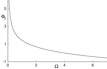
FIG. 3.: The crossover function $\Phi_{2}(\Omega)$ appearing in the local dynamic structure factor.

The longitudinal relaxation rate of nuclei coupled to the electronic spins is $1/T_{1}=(\Gamma/2)S_{+-}(\omega_{N})$, where $\Gamma$ is determined by the electron-nucleus hyperfine coupling, and $\omega_{N}$ is a nuclear frequency which can safely be set to zero. It is useful to explicitly note the $H\ll L_{t}^{-1}$ limit of $1/T_{1}$, where from (21), we have

$$\frac{1}{T_{1}}=\frac{\Gamma T\chi}{\sqrt{2D_{s}H}}=\frac{\Gamma\Delta e^{-3\Delta/2T}}{c^{2}}\sqrt{\frac{3T}{\pi H}}~{}~{};~{}~{}\chi=\frac{e^{-\Delta/T}}{c}\sqrt{\frac{2\Delta}{\pi T}},$$

where $\chi=\lim_{H\rightarrow 0}(\rho_{1}-\rho_{-1})/H$ was known earlier [9, 10]. For experimental comparisons, an important property of the above, pointed out to us by M. Takigawa, is that the low $T$ activation gaps for $1/T_{1}$ ($\Delta_{1/T_{1}}$) and $\chi$ ($\Delta_{\chi}$) satisfy $\Delta_{1/T_{1}}/\Delta_{\chi}=3/2$.

A quantitative comparison of our results with experiments requires a detailed study of the $H$ and $T$ dependencies of $1/T_{1}$, along with consideration of effects due to spin-anisotropies and inter-chain couplings which can become important at low $T$ and $H$. Such an analysis will be presented elsewhere; here, we simply note some trends which appear to receive a natural explanation from our theory. Values for the activation gaps $\Delta_{1/T_{1}}$ and $\Delta_{\chi}$ have been quoted for a number of experimental systems [1, 2, 3], and it has consistently been found that $\Delta_{1/T_{1}}$ is larger than $\Delta_{\chi}$. In the spin $S=1$ chain compound $AgVP_{2}S_{6}$ Takigawa et. al. [1] estimated $\Delta_{1/T_{1}}/\Delta_{\chi}=1.3$; for the spin $S=1$ chain compound $Y_{2}BaNiO_{5}$, Shimizu et. al. [2] measured $\Delta_{1/T_{1}}/\Delta_{\chi}=1.53\pm 0.08$; finally, in the two-leg $S=1/2$ ladder compound $SrCu_{2}O_{3}$, Azuma et. al. [3] found $\Delta_{1/T_{1}}/\Delta_{\chi}=1.6$.

Takigawa et. al. [1] also observed the diffusive $1/\sqrt{H}$ dependence of $1/T_{1}$, from which the value of $D_{s}$ was estimated: $D_{s}/a^{2}\approx 5.5\times 10^{14}$ $\mbox{sec}^{-1}$ at $T=220K$, where $a$ is the lattice spacing. From measurements [17] of $\chi$ we may obtain $\Delta=320K$, and $c/a=3.32\Delta$, which when inserted into (14) give $D_{s}/a^{2}=6.6\times 10^{14}$ $\mbox{sec}^{-1}$. However, it should be noted that numerical analysis [18] on the nearest-neighbor $S=1$ antiferromagnet gives $c/a=6.06\Delta$, but using this value of $c$ would also lead to a discrepancy in the theoretical prediction for $\chi$.

Finally, we note that similar methods [11] can be used to obtain dynamic, $T>0$, correlators of the $n_{\alpha}$ field: this will be described elsewhere.

We are indebted to M. Takigawa for surveying and interpreting the experimental situation for us. We thank Satya N. Majumdar and T. Senthil for stimulating discussions which provoked our interest in this problem, and I. Affleck for helpful remarks. This research was supported by NSF Grant No DMR 96–23181.

REFERENCES

- [1] M. Takigawa et. al., Phys. Rev. Lett. 76, 2173 (1996).
- [2] T. Shimizu et. al., Phys. Rev. B 52, R9835 (1995).
- [3] M. Azuma et. al. Phys. Rev. Lett. 73, 3463 (1994).
- [4] F.D.M. Haldane Phys. Lett. 93A, 464 (1983).
- [5] E.S. Sorensen and I. Affleck, Phys. Rev. B 49, 13235 (1994).
- [6] A.M. Polyakov, Phys. Lett. B 59, 87 (1975).
- [7] A.B. Zamalodchikov and A.B. Zamalodchikov, Ann. of Phys. 120, 253 (1979).
- [8] Form factors in completely integrable models of quantum field theory by F.A. Smirnov, World Scientific, Singapore (1992).
- [9] A.M. Tsvelik, Zh. Eksp. Teor. Fiz. 93, 385 (1987) (Sov. Phys. JETP 66, 221 (1987)).
- [10] J. Sagi and I. Affleck, Phys. Rev. B 53, 9188 (1996).
- [11] S. Sachdev and A.P. Young, preprint cond-mat/9609185.
- [12] A.V. Chubukov, S. Sachdev, and J. Ye, Phys. Rev. B 49, 11919 (1994).
- [13] M. Luscher, Phys. Lett. 118B, 391 (1982).
- [14] Th. Joliceour and O. Golinelli, Phys. Rev. B 50, 9265 (1994).
- [15] D.W. Jepsen, J. Math. Phys. 6, 405 (1965).
- [16] J.L. Lebowitz and J.K. Percus, Phys. Rev. 188, 487 (1969).
- [17] M. Takigawa et. al., Phys. Rev. B 52, R13087 (1995).
- [18] E.S. Sorensen and I. Affleck, Phys. Rev. Lett. 71, 1633 (1993).