Cooperativity and Stability
in a Langevin Model of Protein Folding

Abstract

We present two simplified models of protein dynamics based on Langevin’s equation of motion in a viscous medium. We explore the effect of the potential energy function’s symmetry on the kinetics and thermodynamics of simulated folding. We find that an isotropic potential energy function produces, at best, a modest degree of cooperativity. In contrast, a suitable anisotropic potential energy function delivers strong cooperativity.

Introduction

Physical chemists have long marvelled at the ability of globular proteins to fold quickly from a random denatured state to a specific three-dimensional conformation. Though much has been learned about this phenomenon since then, we still lack a satisfactory theory of the folding process.

Theoretical work in this area has, from the beginning, relied heavily on computer simulations. The early efforts to model protein folding numerically attempted to represent real proteins for which crystallographic and other experimental data were available. This type of simulation study, which is still much used today, starts with as realistic a representation of the modelled protein and the physical interactions between its constituents as is computationally affordable. We may describe this as a “top-down” approach. In contrast, a more recent approach proceeds from the bottom up. It starts with the simplest model that still bears a minimal resemblance to a protein while still being complex enough to pose non-trivial theoretical questions. The most important examples of this strategy are the lattice models of protein folding (e.g. [1, 2, 3, 4, 5]). These models reduce the protein to a linear self-avoiding chain of beads that are constrained to inhabit points in a discrete three-dimensional lattice; the kinetics and the thermodynamics features of the models are accordingly streamlined. These very simple lattice models have allowed researchers to tackle theoretical questions that are computationally prohibitive to top-down models.

Despite their great usefulness, however, the extreme simplicity of lattice models gives rise to the legitimate question of how much the results obtained with lattice models depend on the severe geometric constraints imposed by the lattice. Moreover, these very constraints preclude the investigation of important questions that are too sensitive to finer geometric details than can be represented in discretized space. Therefore, both to independently test the results obtained by lattice models, and to address questions sensitive to fine geometrical details, it would be useful to have simple off-lattice models of protein folding. A few investigators have produced such models, and obtained encouraging results (e.g. [6, 7, 8, 9]). One aspect that these previous studies have not fully addressed, however, is the degree of cooperativity observed in the unfolded $\leftrightarrow$ folded transition. This question is the focus of the present work.

Model

We model proteins as linear self-avoiding chains of hard spheres (corresponding roughly to amino acids) connected by rigid rods (corresponding roughly to $C_{\alpha}-C_{\alpha}$ pseudobonds). Except for the excluded-volume constraints imposed by the hard spheres, the chain is freely jointed at each monomer.

We use the basic strategy of classical molecular dynamics algorithms: at each time step, each monomer is displaced slightly, according to the forces acting on it. The net force on each monomer is the sum of a “regular” component, derived from the potential energy field generated by nearby monomers, and a “random” or “noise” component, drawn randomly from a Maxwell distribution. Our displacements are computed according to Langevin’s equation of motion in a viscous medium. (For more details on the use of Langevin dynamics to model protein motion, consult [9] and  [7]. Many aspects of our algorithm derive from the one presented in [9]. One important difference is our use of a SHAKE algorithm to enforce bond-length constraints, thereby avoiding the bond-length divergence as $t\rightarrow\infty$ reported in that work.)

For any chain configuration, the potential energy $U$ is computed as

$$U=\sum_{i=1}^{N-2}\sum_{j=i+2}^{N}U_{ij},$$ (1)

where $U_{ij}$ is the potential energy of the pair $ij$ of monomers.

In addition to the hard-sphere repulsion between all pairs of monomers, there is also a short-range attraction between those monomers that are in contact in the native conformation. (The precise definition of a native contact is given below.) The strength of this attraction is the same for all such pairs. (This aspect of the model is entirely analogous to that proposed by Go et al. in [10], and hence we refer to it as “the Go prescription.” This class of models may be viewed as the limiting case for optimal design in more realistic “sequence” models, i.e. models in which the pairwise energies of interaction depend on the chemical identity of the interacting residues.) Hence, the potential energy function, in general, consists of a repulsive part and an attractive part, the latter being zero for all but those monomer pairs that form native contacts. The two variants of our model presented in this paper differ solely in the function used to represent the attractive part of the potential acting at native contacts. In one model, this attractive potential is spherically symmetric, whereas in the other it is completely asymmetric. In this paper, we will refer to them as the “isotropic” and “anisotropic” models, respectively.

We describe the potential energy function used in the isotropic model via the expression for the terms $U_{ij}$ in Equation 1:

$$U_{ij}(r)=U_{0}\left[\left(\frac{r_{0}}{r}\right)^{12}-2\Delta_{ij}\left(\frac{r_{0}}{r}\right)^{6}\right]$$ (2)

Except for the term $\Delta_{ij}$ on the right, this is a standard Lennard-Jones 6-12 potential. We define $\Delta_{ij}$ to be 1 if monomers $i$ and $j$ are within a distance of 2 bond-lengths of each other in the native structure (i.e. they constitute a native contact for the purpose of Go’s prescription); otherwise $\Delta_{ij}=0$.

To write the corresponding expression for the anisotropic model we must first define one additional variable, namely the angle $\theta$ shown in Figure 1. Starting from an arbitrary Cartesian representation of the native structure, for each pair $i,j$ of monomers that form a contact in this reference native structure (using the distance criterion given in the previous paragraph), we define a unit vector ${\bf\hat{u}}_{ij}$ pointing from monomer $i$ to monomer $j$, and, conversely, another unit vector ${\bf\hat{u}}_{ji}=-{\bf\hat{u}}_{ij}$ in the opposite direction. For the sake of computational efficiency, in the version of our anisotropic model presented here, once the orientations of these unit vectors are defined at the start of the simulation, they remain constant throughout. (In a more general model, these vectors would be free to rotate, as long as all the unit vectors emanating from a given monomer rotated together as a rigid body, i.e. preserving all the angles between them; for further remarks on this important aspect of the model see the Discussion section.) Now, we define the angle $\theta\in[0,\pi]$ as that between the unit vector ${\bf\hat{u}}_{ji}$ (or, equivalently, ${\bf\hat{u}}_{ij}$) and the line connecting monomers $i$ and $j$ (see Figure 1). It measures the deviation of the $ij$ couple’s (signed) orientation from what it is in the native state. For the sake of completeness, if monomers $i$ and $j$ do not participate in a native contact, we define $\theta=0$. Now we can write the expression analogous to Equation 2 for the anisotropic case:

$$U_{ij}(r,\theta)=U_{0}\left[\left(\frac{r_{0}}{r}\right)^{12}-2\Delta_{ij}\left(\frac{r_{0}}{r}\right)^{6}e^{-6\theta^{2}}\right].$$ (3)

Figure 1: Definition of the $\theta$ angle, used in Equation 3.

The new element in this expression is the test function $e^{-6\theta^{2}}$ used to penalize deviations of $\theta$ from zero .

Methods

The overall structure of the algorithm we use is standard: at every time step, random forces are generated and regular forces computed; from these, the unconstrained displacements are computed; finally, we use a SHAKE [11, 12] subroutine to enforce bond-length constraints.

The 3 spatial components of the random force ${\bf F}_{rand,i}$ on monomer $i$ are independently generated as normally distributed random variables with zero mean and variance $2D/\Delta t=2k_{B}T/\gamma\Delta t$, where $D=k_{B}T/\gamma$ is the diffusion coefficient, $k_{B}$ the Boltzmann constant, $T$ the temperature, $\gamma$ the frictional drag coefficient, and $\Delta t$ the simulation’s time-step. This choice of variance for the forces ensures that, in the absence of regular forces, the variance of the resulting displacement will be $6D\Delta t=3\times 2k_{B}T\Delta t/\gamma$. We rescale to dimensionless parameters, setting $k_{B}=1$ and $\gamma=1$; therefore, the diffusion coefficient becomes numerically equal to the temperature. With these definitions, one time unit corresponds to the time it takes, at $T=1$, for a particle to diffuse, on average, a distance of $\sqrt{6}\approx 2.45$ bond lengths. In our simulations we use a time step $\Delta t$ never greater than 0.001 time units.

The contribution to the regular force produced by monomer $j$ on monomer $i$ is computed as $-\nabla U_{ij}$. For the following exposition, we rewrite Equations 2 and 3 as

$$U_{ij}(r,\theta)=U_{0}\left[\left(\frac{r_{0}}{r}\right)^{12}-2\Delta_{ij}\left(\frac{r_{0}}{r}\right)^{6}A(\theta)\right]$$ (4)

(where now equations 2 and 3 may be recovered from equation 4 by setting $A(\theta)=1$ and $A(\theta)=e^{-6\theta^{2}}$, respectively). We set $U_{0}=1$, and therefore, $U_{0}$ may be regarded as our energy unit. Likewise, we use the bond length as our basic unit of distance (although occasionally we use the conversion 1 bond length = $C_{\alpha}-C_{\alpha}$ distance = 3.8 Å, to make our results more directly comparable to experimental values). To ensure that the chain does not cross itself, we make such crossings energetically prohibitive by setting $r_{0}=1.5$ bond lengths.

Evaluating $-\nabla U_{ij}$ in local polar coordinates at $(r,\theta)$, we get

$${\bf F}_{ij} = -\left(\frac{\partial U_{ij}}{\partial r}\,{\bf\hat{r}}+\frac{1}{r}\,\frac{\partial U_{ij}}{\partial\theta}\,{\bf\hat{\mbox{\boldmath$\Theta$}}}\right)$$

$$= 12\;U_{0}\left(\frac{r_{0}^{12}}{r^{13}}-\frac{\Delta_{ij}r_{0}^{6}}{r^{7}}A(\theta)\right){\bf\hat{r}}+\frac{2U_{0}\Delta_{ij}r_{0}^{6}}{r^{7}}A\,^{\prime}(\theta){\bf\hat{\mbox{\boldmath$\Theta$}}},$$

where the terms $r,\theta,{\bf\hat{r}}$, and ${\bf\hat{\Theta}}$ are as shown in Figure 1. In particular, ${\bf\hat{r}}$, and ${\bf\hat{\Theta}}$ are orthogonal unit vectors. The latter is coplanar with ${\bf\hat{u}}_{ji}$ and ${\bf\hat{r}}$. (Of the two directions that ${\bf\hat{\Theta}}$ can have, and still be both orthogonal to ${\bf\hat{r}}$ and coplanar with ${\bf\hat{u}}_{ji}$ and ${\bf\hat{r}}$, we have chosen the one along which moving monomer $i$ increases $\theta$; see Figure 1).

Note that in the isotropic case, $A\,^{\prime}$ is identically zero, so the regular force consists of a radial component only. In the anisotropic case, on the other hand, $A\,^{\prime}(0)=0$, and $A\,^{\prime}(\theta)<0,\,\forall\,\theta\in(0,\pi)$.

The total regular force ${\bf F}_{reg,i}$ on monomer $i$ is simply

$${\bf F}_{reg,i}=\sum_{j\ni|j-i|\geq 2}^{N}{\bf F}_{ij},$$

(In fact, for the sake of computational speed, the algorithm ignores the contributions to the regular force from monomers outside of a cutoff radius $r_{\mbox{\scriptsize cutoff}}=1.8\,r_{0}=2.7$.)

We obtain the total force ${\bf F}_{i}$ on monomer $i$ from

$${\bf F}_{i}={\bf F}_{rand,i}+{\bf F}_{reg,i},$$

and the corresponding (unconstrained) displacement $\Delta{\bf R}_{i}$ from

$$\Delta{\bf R}_{i}=\Delta t\;{\bf F}_{i},$$

The above expression comes from the Langevin equation [13]:

$$\gamma{\bf v}_{i}+m_{i}\frac{d{\bf v}_{i}}{dt}={\bf F}_{i}$$

($\gamma=$ frictional drag coefficient; ${\bf v}_{i}=$ velocity of $i$th monomer) with the further assumption that the inertial term $m_{i}\frac{d{\bf v}_{i}}{dt}$ is negligible:

$$\frac{m_{i}}{\gamma}\frac{d{\bf v}_{i}}{dt}\approx 0.$$

In the present work we have set $\gamma=1$. Hence

$$\Delta{\bf R}_{i}=\Delta t\;{\bf v}_{i}=\Delta t\left(\frac{1}{\gamma}\right){\bf F}_{i}=\Delta t\;{\bf F}_{i}.$$

Finally, the new unconstrained positions ${\bf R}_{i,unc}={\bf R}_{i,old}+\Delta{\bf R}_{i}$ are submitted to a standard SHAKE routine [11] to enforce bond-length constraints. For the SHAKE routine, we used a tolerance of 0.01 times the bond-length squared [12].

We obtained our native structures by simulating homopolymer collapse, with a penalty for contacts between neighboring residues along the chain (more specifically, between residues $i$, $j$ satisfying $|i-j|=2$).

Results

The isotropic model described in the Model section above succeeded in folding model proteins of up to length 70 (the longest we studied). A typical folding trajectory for a 70-mer is shown in Figure 2.

Figure 2: Typical folding trajectories for one 70-mer, using the isotropic (solid line) and anisotropic (dashed line) models. For both trajectories $T=0.6$.

To study the nature of the unfolded $\leftrightarrow$ folded transition, we focused on the behavior of one particular 30-mer (s30.1). This structure was obtained by homopolymer collapse at a low temperature, followed by a very brief period of steepest-descent energy minimization. It contains 111 native contacts, and has a native-state energy of -88.7. Moreover, its radius of gyration is 1.77, which is close to maximally compact for a 30-mer.

To gauge the degree of cooperativity in the transition between the folded and the unfolded states, we first determined the transition temperature for this structure to be $T_{f}\approx 0.64$. We then collected a long time series, at this temperature, of the distance RMSD and the energy (Figure 3), as well as the fraction of native contacts ($Q$, data not shown). A histogram plot of the enthalpies collected during this trajectory (cf. Figure 4) and the corresponding frequency tallies (cf. Figure 5) of the fraction of native contacts ($Q$), show only a modest degree of cooperativity for the isotropic model.

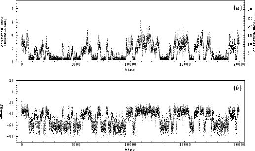
Figure 3: Long folding trajectory at $T=0.64\approx T_{f}$, using the isotropic model. The top graph ($a$)shows distance RMSD vs. time (scale on the left is normalized, or bond-length, units; the scale on the right is in angstroms). The bottom graph ($b$) shows energy vs. time.

Figure 4: Distribution of energies for trajectory shown in Figure 3.

Figure 5: Frequencies of $Q$-values ($Q$ = fraction of native contacts) for trajectory shown in Figures 3.

To determine how much the above results depended on chain length, we performed a similar analysis for three different 65-mers. The first of these was obtained from the $C_{\alpha}$ trace of chymotrypsin inhibitor 2 (CI2). The second and third (s65.2 and s65.3) were obtained by homopolymer collapse at a low temperature, though for the third one, the collapse was carried out for a longer period of time than for the second one, resulting in a more compact structure. Various relevant measurements for these three structures are given in Table 1. Histograms for the energy time-series for each structure (near their respective transition temperatures) are shown in Figure 6.

structure	CI2	s65.2	s65.2
gyration radius	2.88	2.63	2.32
native-state energy	-49.5	-233	-241
approximate $T_{f}$	0.54	0.74	0.81
number of native contacts	188	306	328
median $|i-j|$ for native contacts	4.5	8	10

Table 1: Summary of physical characteristics of the three 65-mers investigated.

(a) CI2

(b) s65.2

(c) s65.3

Figure 6: Energy distribution near $T_{f}$ for three 65-mers.

In the best case, that of structure s65.3, we see only a slightly stronger cooperativity (as judged by the histograms’ peak/trough height ratios) than observed with the 30-mer s30.1 (compare with Figure 4). It is interesting to see, however, that the other two cases exhibit very little or no cooperativity at all. The CI2 structure is somewhat anomalous relative to the other two 65-mers, as shown in Table 1. It has by far the highest energy, not only for having the fewest native contacts, but also for having a few strongly repulsive ones (the monomers involved are slightly closer to each other than the hard-sphere distance). Moreover, most of its contacts are between monomers that are relatively close to each other along the chain. As has been demonstrated with lattice models [14], an abundance of such “local” contacts weakens the cooperativity of the transition. It is suggestive that the median value, over all native contacts, of their degree of “locality” $|j-i|$ (where $i$ and $j$ are the positions along the chain of the residues in the contact) reflects the observed degree of cooperativity, at least within this limited sample (cf. Table 1).

We also looked at the effect of native-state stability $\Delta F/T$ on median first-passage time for the 30-mer s30.1. (We estimated the relation between the native-state stability and the inverse temperature using the “histogram method” proposed by Ferrenberg and Swendsen in [15].) The results are shown in Figure 7 , where each data point represents the median folding time of 50 folding simulations. It is noteworthy that the optimal median folding time is below 100 time units, but the flattening of the curve and the data’s noise preclude a satisfactory determination of an optimal native-state stability for folding.

Figure 7: Dependence of first-folding time on native-state stability ($\frac{\Delta F}{k_{B}T}$) for isotropic model. The curve shown (solid line) is the sample median (50 observations per native-state stability). We used a cutoff of 1000 time units for these simulations. The integers shown above the dotted line at this cutoff represent the numbers of runs, at the corresponding native-state stabilities, that did not result in a folded structure within the cutoff period (omitted when equal to zero).

Spurred by the relatively weak degree of cooperativity shown by the isotropic model, we devised the anisotropic model described in the Model section above. This model, too, was capable of folding proteins of up to 70 residues in length (the longest we attempted). A sample folding trajectory for a 70-mer is shown in Figure 2.

We performed the same analyses as those performed with the isotropic model, again using as our test structure the 30-mer s30.1. A long trajectory at $T_{f}\approx 0.725$ is shown in Figure 8. The corresponding histogram of enthalpies and tally of Q-value frequencies (Figures 9 and 10) show a considerably greater degree of cooperativity than observed with the isotropic model. To further quantify the strength of the first order transition, we plotted the heat capacity $C\equiv dU/dT$ vs. $T$ (Figure 11), computed via the histogram method [15] from the data shown in Figures 3 and 8. The maximum heat capacity for the anisotropic model is almost 5 times greater than for the isotropic one. We estimated the transition barrier for each model, from the data shown in Figures 5 and 10; we obtained roughly 2 $k_{B}T$ and 6 $k_{B}T$, for the isotropic and anisotropic models, respectively.

The effect of native-state stability on first-passage time is shown in Figure 12. As was the case with the isotropic model, the curve flattens in the high-stability region, which, combined with the data’s noise precludes an adequate estimation of the native-state stability optimal for folding. Taking into account these caveats, we may estimate that the optimal median folding time in this case is probably below 500 time units, certainly below 1000.

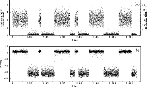
Figure 8: Long folding trajectory at $T=0.725\approx T_{f}$, using the anisotropic model. The top graph ($a$) shows distance RMSD vs. time (scale on the left is normalized, or bond-length, units; the scale on the right is in angstroms). The bottom graph ($b$) shows energy vs. time.

Figure 9: Distribution of energies for trajectory shown in Figure 8.

Figure 10: Frequencies of $Q$-values for trajectory shown in Figure 8.

Figure 11: Heat capacity ($C$) vs. temperature for the isotropic and anisotropic models.

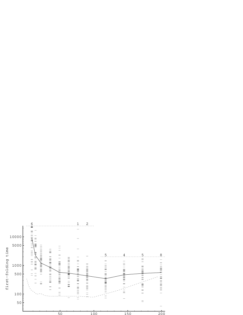
Figure 12: First passage times as a function of native-state stability ($\frac{\Delta F}{k_{B}T}$), for anisotropic model. The upper curve (solid line) is the sample median (50 observations per native-state stability). For these simulations, we used cutoffs of 24,000 and 2,000 time units, for the low and high native-state stability regions, respectively, as indicated by the horizontal dotted lines. The integers shown above these dotted lines represent the numbers of runs, at the corresponding native-state stabilities, that did not result in a folded structure within the indicated cutoff period; omitted when equal to zero. The dotted curve appearing at the lower left is the same median curve presented in Figure 7; it is shown here for reference.

We further investigated the nature of 30-mer s30.1’s unfolded state near $T_{f}$ under the isotropic and the anisotropic models. As Figure 13 shows, the histogram for the radius of gyration of the unfolded state in the anisotropic model is around 4, almost indistinguishable from that of a simple self-avoiding chain (i.e. one with no interaction between monomers other than hard-sphere repulsion). In contrast, with the isotropic model, the unfolded state’s mean radius of gyration is approximately 3. Hence, with the isotropic model, this 30-mer is never fully extended, at least at $T\approx T_{f}$; instead, it remains in a somewhat compact globular state.

For both models, at high native-state stabilities (low temperatures) kinetic traps became increasingly common. Each model, however, exhibited traps of a characteristic type. In the isotropic model, for all the cases examined, the kinetically trapped structures consisted of two well-folded domains of opposite chirality. In the anisotropic model chiral traps were never observed, as would be expected, since, contrary to the isotropic model, the anisotropic one discriminates between enantiomers. Instead, almost all of the trapped structures we observed with the anisotropic model were what we could call “dumbbell” traps: two perfectly folded halves that were, however, ill-positioned with respect to one another. The two exceptions we found to this pattern were structures that were almost completely folded except for short loops, towards the middle of each chain, that could not attain their final buried positions due to the tightness of the rest of the folded chain. It is important to point out, however, that for both models, kinetic traps were observed only at native-state stabilities 3-15 times greater than those typical of real proteins.

As would be expected, the two models also differ in the rigidity they confer to the native state. Figure 14 shows that, at all native-state stabilities, the native state of the 30-mer s30.1 is significantly more rigid with the anisotropic model.

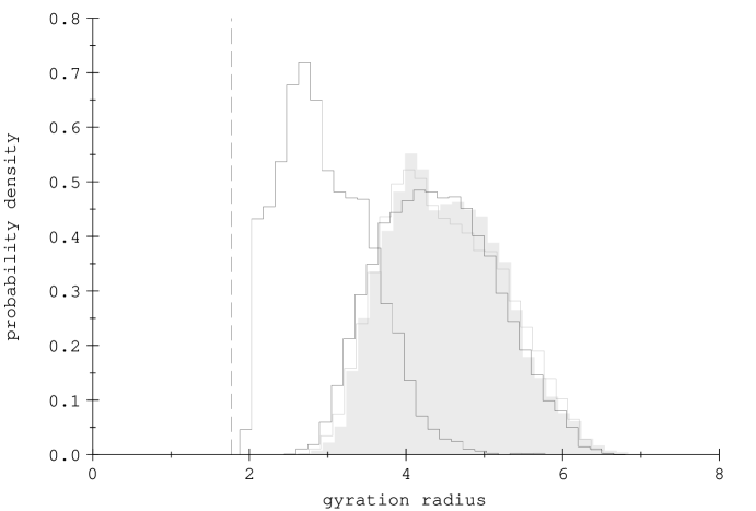
Figure 13: Distribution of radii of gyration. The hump on the left corresponds to the unfolded state under the isotropic model, at $T=0.64$. The filled histogram on the right corresponds to the distribution resulting from turning off all attractive potentials, at $T=0.64$. The (unfilled) histogram on the right with dark gray borders was obtained under the same conditions as the filled histogram, but with $T=0.725$. Finally, the remaining (black-edged, unfilled) histogram on the right corresponds to the unfolded state under the anisotropic model, at $T=0.725$. The dashed line on the left marks the radius of gyration (1.77) of the native structure. (For reference, bonds have unit length, and the potential energy minima are at $r_{0}=1.5$.)

Figure 14: Mean distance RMSD for the folded chain, as a function of the native-state stability.

Discussion

We have presented two simple off-lattice models of protein folding, which we have called the “isotropic” and “anisotropic” models, respectively, in reference to the potential energy functions they use. Although both models achieve the primary requirement of folding model proteins (up to length 70, at least) to their native states, they show several substantive differences. These are summarized in Table 2.

model	isotropic	anisotropic
first-order transition	weak	strong
optimal median folding time ($t_{\mbox{\scriptsize opt}}$)	(70)	(350)
(median folding time at $T_{f}$) $\div\;t_{\mbox{\scriptsize opt}}$	(5)	$(10^{2}-10^{3})$
gyration radius of unfolded state: mean and (sd)	3.1 (0.55)	4.4 (0.73)
rigidity of native state	low	high
type of kinetic traps	chiral	dumbbell

Table 2: Summary of functional differences in the folding of one 30-mer between the isotropic and anisotropic models.

Our analysis of the folding transition for the isotropic model showed that it was capable of delivering a modest, but detectable, degree of cooperativity. From the data shown in Figure 5, we estimate a barrier of 1-2 $k_{B}T$ at $T\approx T_{f}$. Guo and Brooks [16] have obtained very similar results in their study of the off-lattice model first proposed in [6, 7]. This relatively weak first order transition delivered by the isotropic model was the primary motivation behind our development of the anisotropic one. The plot of energy vs. distance RMSD at $T\approx T_{f}$ for the isotropic model (Figure 15) suggested to us that its spherically symmetrical potential energy function resulted in the relative stabilization of a sizeable population of states (namely, those in the region defined by a distance RMSD $>$ 0.9 bond lengths $\approx$ 3 Å, and energy $<$ -43), that were unrelated to the native one. This, in turn, would promote a non-cooperative component to the folding mechanism: the gradual rearrangement of a partially collapsed unfolded state.

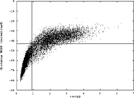
Figure 15: Energy vs. Distance RMSD plot for the data shown in Figure 3.

We then hypothesized that rigidly asymmetric potentials would lead to cooperative folding. To illustrate the reasoning behind this hypothesis, we propose a simple example in two dimensions. Consider first a system of identical circular particles (see Figure 16) performing Brownian motion within a bounded 2-dimensional space. Suppose that these particles have 6 hexagonally arranged “interaction sites,” such that any two such sites on different particles attract each other. Let the change in energy upon formation of one such contact be $\Delta U<0$, and the corresponding change in entropy (upon fixing of one particle relative to the other) be $\Delta S<0$. Therefore, starting from a “monoatomic” state (i.e. all particles unattached) at temperature $T$, the formation of the first pairwise contact entails a free-energy change $\Delta F=\Delta U-T\Delta S$. However, the very formation of this first contact creates two new “composite” interaction sites (labeled 1 and 2 in Figure 16), each consisting of two simple sites. The crucial point is that now the arrival of a third monomer at one of these new composite sites entails a free-energy change of $2\Delta U-T\Delta S<2\Delta F$. Therefore, at any temperature, it is thermodynamically more favorable to form two new contacts by adding a third monomer to the dimer at one of the new composite sites, than by bringing together two separate pairs of monomers (as would happen if monomers attached at sites 3 and 4, for example). As a consequence, in this system, the fixed geometrical arrangement of a discrete set of attachment sites on each monomer to cooperative aggregation. We use the term steric nucleation to refer to this interplay between the thermodynamics of contact-cluster formation and the geometrical arrangement of the interaction sites on each monomer.

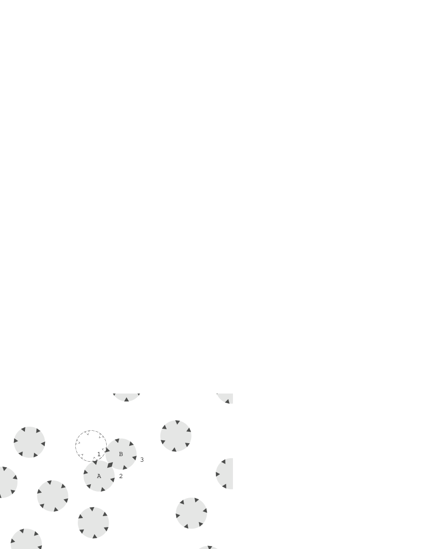
Figure 16: Circular particles with hexagonal arrangement of interaction sites. The formation of a contact between particles A and B simultaneously produces composite interaction sites 1 and 2.

Now, we consider a hypothetical protein. Let us suppose that its native state includes a “triangular” set of contacts between monomers $i$ and $j$, $j$ and $k$, and $i$ and $k$. (We will refer to this as a “3-cluster,” short for “3-contact cluster”). Furthermore, suppose that, like in the 2D example above, the very formation of any one of these three contacts orients the two participating monomers in such a way that the subsequent arrival of the third monomer results in the simultaneous formation of the cluster’s remaining two contacts. Then, reasoning as before, we expect that the formation of this contact cluster will be cooperative. Taking this reasoning one step further, we see that if a native structure consisted of an interconnected network of such $n$-clusters ($n\geq 3$), then the entire folding event would be cooperative.

It is plausible that some form of steric nucleation contributes to the cooperativity observed in the folding of real proteins. Since amino acids are completely asymmetrical molecules, we expect that, in general, the change in energy resulting from bringing two of them together will depend not only on the distance between them, but also on their relative orientations. This would mean that the energy landscape for the interaction between two amino acids would feature a few discrete minima. In the language used above, protein optimization may involve assembling $n$-clusters of spatially complementary contacts into an interconnected network spanning the entire native structure. To be sure, it is unlikely that all, or even most, of the intramolecular interactions contributing to the energy of folding of a real protein are as narrowly specific as the active contacts built into our anisotropic model. A more realistic possibility is that, in a real protein, only a fraction of these interactions have the steric stringency of the anisotropic model, but that, nonetheless, these alone are sufficient to render the folding cooperative. This hypothesis immediately proposes the investigation of a hybrid model, in which some contacts are sterically restricted, while others are not. More precisely, we may ask, what is the relation between the fraction and/or strength of contacts that are sterically restricted, and the degree of cooperativity of the folding transition? And can a small subset of such contacts serve as a specific nucleus for the folding of the whole chain? Another interesting study would be of the structures of proteins homologous to one of those for which a folding nucleus has been experimentally identified, to see if the residues corresponding to nucleus sites exhibit a greater degree of spatial overlap across the various homologs than would be otherwise expected. These are investigations we are currently pursuing.

We devised the anisotropic model as a simple modification of the isotropic one that would be capable of specifically testing the steric nucleation hypothesis presented above, within the context of off-lattice model-protein folding. We believe it has served this purpose well. However, in the name of expediency and computational efficiency, for its implementation we chose to keep all the sets of vectors ${{\bf\hat{u}}_{ij}}$ (cf. Model section) at fixed, concordant orientations throughout the simulation. It is likely that the greater first-folding times of the anisotropic model are due, at least in part, to this feature of our implementation. Indeed, the latter implies that any rotation of the native structure, or more importantly, of any small fragment thereof, will be destabilizing. This, in turn, implies a higher kinetic barrier for the anisotropic model than would be expected for a model that did not impose a fixed spatial orientation on the native state. A more generally applicable implementation of the anisotropic model than the one we chose would have allowed all the vectors ${\bf\hat{u}}_{ij}$, for any given monomer $i$, to rotate together as a rigid unit, and independently of any other set ${\bf\hat{u}}_{i\,^{\prime}\,j}$. Such a model would still support steric nucleation, but it would also allow $n$-clusters to form in several spatial orientations that would, in general, would be all different from each other. Therefore, even though such a model would give each pair of monomers 3 more degrees of freedom, thereby reducing the probability of nucleus formation, those nuclei that did form would be much less fragile than those in our version here. Hence, it is possible that, despite the increase in the size of the chain’s conformational space, such a generalized model would result in faster folding times.

Incidentally, it is worth remarking that for a 30-mer on a cubic lattice, and still using a Go-type model, the optimal median folding time is about 27000 Monte Carlo steps [17]; upon dividing this figure by the chain length (to correct for the difference in the counting of time between the Monte Carlo methods and the off-lattice methods presented here), we get 900 time units, or roughly 1 order of magnitude slower than for the optimal median folding time isotropic model. This slowness of the lattice relative to the isotropic model probably reflects the lattice’s much more limited geometry.

It is clear from the energy trajectory in Figure 3 (or from Figure 4) that with the isotropic model, a significant fraction of the native contacts are present in the unfolded state (for both models, the energy of a perfectly stretched conformation is zero). Moreover, with the isotropic model the unfolded state is significantly more compact, as measured by the radius of gyration, than it is with the anisotropic model. With the anisotropic model, on the other hand, the energy of the unfolded state is slightly above zero, consistent with very few native contacts (and a few unfavorable hard-ball repulsions). Indeed, we found that, at $T\approx T_{f}$, with the isotropic model the average value for the fraction $Q$ of native for the unfolded state was between 0.4 and 0.5, whereas with the anisotropic model this figure was below 0.1. (See Figures 5 and 10.) Moreover, for the latter, $Q-$values between 0.3 and 0.6 are almost never observed. These data suggest that, in the anisotropic model, the transition state for the structure under study consists of conformation(s) with about $30\%$ of the native contacts. (Further study will reveal how specific this $30\%$ needs to be to ensure folding.) In contrast, the corresponding figures for the isotropic model suggest that when pairwise distance is the only requirement for contact formation, there are many unproductive ways of making contacts (Figure 5). Finally, in relation to the foregoing, we should note that the anisotropic model seems to recapture one of the features of the lattice that was lost by the isotropic model, namely a very small number of ways in which $n$-clusters may form. While the lattice features anisotropy inherently, it must be explicitly introduced into off-lattice models.

We should also note that it is possible that the relative compactness of the unfolded state in the isotropic model contributes to its greater folding speed. True, with the isotropic model, there appears to be a greater likelihood that the chain will spend time sampling unproductive conformations of relatively low energy. However, even at modest native-state stabilities, the isotropic model folds within a mere one hundred time units. Thus, it is possible that the net effect of compactization is to enhance folding rate. Further investigation is necessary to sharpen our understanding of this matter.

Folding was generally faster with the isotropic model than with the inosotropic one at all native-state stabilities studied, although the difference becomes negligible (to within the data’s noise) at the highest native-state stabilities. As just alluded to, with the anisotropic model, the chain is not as likely to linger in misfolded states of relatively low energy, as it is with the isotropic model. On the other hand, with the anisotropic model, contact formation will certainly be more infrequent than with the isotropic model, since, with the former, and not with the latter, contact formation requires residues to approach each other in a precise orientation. It appears (Figure 12) that the latter effect dominates the kinetics of the anisotropic model, at least for most of the range of native-state stabilities studied. Interestingly, with both models, the median folding time curves plateau at high native-state stabilities (Figures 7 and 12). We hypothesize that this is an artifact of Go’s prescription. Indeed, in a sequence model energetically favorable non-native contacts are possible, which would result in a faster increase in median folding time as a function of increasing native-state stabilities than with the models presented here.

It is at temperatures close to $T_{f}$, however, that the two models presented here differ most dramatically. For the isotropic model, the ratio of the folding time at the transition temperature $T_{f}$ and the optimal folding time $t_{\mbox{\scriptsize opt}}$ is roughly 5. For the anisotropic model, we cannot give a similarly precise figure, due to our inability to collect adequate statistics for this model at $T_{f}$. However, it is clear from our experience so far with this model (typified by the time course in Figure 8) that this ratio is well above 100, and probably lies somewhere between 300 and 1000. This difference can be seen as indicative of the greater role of nucleation in the anisotropic model, since the rate of nucleus formation is very sensitive to high temperatures.

In this connection, it is interesting to note a very remarkable property of real proteins, namely that their folding rate decreases by up to three orders of magnitude as the stability of the native state is reduced to zero [18, 19, 20]. In light of this experimental fact, it is encouraging to see that the anisotropic model produces a commensurate retardation of folding at zero native-state stability. Our enthusiasm is tempered, however, upon noting that real proteins achieve this retardation over a range of native-state stabilities of only 10-20 $k_{B}T$, while with our anisotropic model it occurs over a 10-fold greater range. Although we expect to see a significant change in folding kinetics once we generalize the anisotropic model (to allow freely rotating contacts), it is not immediately clear how this generalization will affect either the range of folding rates, nor the corresponding range of native-state stabilities.

References

- [1] A. S̆ali, E. Shakhnovich, and M. Karplus, Nature 369, 248 (1994).
- [2] H. S. Chan and K. A. Dill, Journal of Chemical Physics 100, 9238 (1994).
- [3] E. I. Shakhnovich, Physical Review Letters 72, 3907 (1994).
- [4] M.-H. Hao and H. A. Scheraga, Journal of Physical Chemistry 98, 4940 (1994).
- [5] N. D. Socci and J. N. Onuchic, Journal of Chemical Physics 101, 1519 (1994).
- [6] J. D. Honeycutt and D. Thirumalai, Proceedings of the National Academy of Sciences USA 87, 3526 (1990).
- [7] J. D. Honeycutt and D. Thirumalai, Biopolymers 32, 695 (1992).
- [8] H. Grubmüller and P. Tavan, Journal of Chemical Physics 101, 5047 (1994).
- [9] N. Grønbech-Jensen and S. Doniach, Journal of Computational Chemistry 15, 997 (1994).
- [10] H. Taketomi, Y. Ueda, and N. Go, International Journal of Peptide and Protein Research 7, 445 (1975).
- [11] J.-P. Ryckaert, G. Ciccoti, and H. J. C. Berendsen, Journal of Computational Physics 23, 327 (1977).
- [12] K. D. Hammonds and J.-P. Ryckaert, Computer Physics Communications 62, 336 (1991).
- [13] D. A. McQuarrie, Statistical Mechanics, HarperCollins, 1976.
- [14] V. I. Abkevich, A. M. Gutin, and E. I. Shakhnovich, Journal of Molecular Biology 252, 460 (1995).
- [15] A. M. Ferrenberg and R. H. Swendsen, Physical Review Letters 61, 2635 (1988).
- [16] Z. Guo and C. L. Brooks, III, (1996), (Submitted for publication).
- [17] A. M. Gutin, V. I. Abkevich, and E. I. Shakhnovich, Physical Review Letters (1996), (Submitted for publication).
- [18] S. E. Jackson and A. R. Fersht, Biochemistry 30, 10428 (1991).
- [19] S. Khorasanizadeh, I. D. Peters, T. R. Butt, and H. Roder, Biochemistry 32, 7054 (1993).
- [20] L. S. Itzhaki, D. E. Otzen, and A. R. Fersht, Journal of Molecular Biology 254, 260 (1995).