Linear stability analysis of the Hele-Shaw cell with lifting plates

Abstract

The first stages of finger formation in a Hele–Shaw cell with lifting plates are investigated by means of linear stability analysis. The equation of motion for the pressure field (growth law) results to be that of the directional solidification problem in some unsteady state. At the beginning of lifting the square of the wavenumber of the dominant mode results to be proportional to the lifting rate (in qualitative agreement with the experimental data), to the square of the length of the cell occupied by the more viscous fluid, and inversely proportional to the cube of the cell gap. This dependence on the cell parameters is significantly different of that found in the standard cell.

]

I Introduction

Despite of the great effort devoted lately to improve the understanding of Saffman-Taylor (ST) instabilities[2, 3], many related experimental facts still lack a sound explanation [4]. Here we are interested in the experimental observations on Hele-Shaw (HS) cells with lifting plates[5]. This variation with respect to the standard constant gap HS cell was suggested as a way to bring the ST problem closer to directional solidification [6, 7]. In this experiment (see Fig. 1), instead of applying pressure to the less viscous fluid, the upper plate is lifted at the less viscous side (commonly air) at a fixed rate. It seems clear that the lifting of the upper plate will promote a pressure gradient analogous to the temperature gradient present in directional solidification. An interesting variation of this experiment is the Hele–Shaw cell with a small gap gradient investigated by Zhao et al[8].

The main results of the work reported by Ben–Jacob et al[5] concern the spacing of the dendrites. These authors observed that this spacing decreased as the lifting velocity was increased. They also noted a dependence on the initial plate spacing. On the other hand, although the experimental results for the HS with lifting plates have been analysed by means of a simplified version of the growth law [9, 10], a detailed analysis of this system is still lacking.

In this work we present a study of growth instabilities in Hele–Shaw cells with lifting plates. We first derive the basic equation (growth law), which results to be different from that proposed by Ben–Jacob et al [5]. In particular our equation is not homogeneous, and thus the comparison with the simpler version of the directional solidification problem is not so evident. Then we discuss the boundary conditions and carry out the linear stability analysis. Our results qualitatively explain the experimental data reported by Ben–Jacob et al [5].

II Basic equations and boundary conditions

Flow in the Hele-Shaw cell is governed by the Navier-Stokes equation [11, 12]

$$\frac{\partial{\bf v}}{\partial t}+({\bf v}.{\bf\nabla}){\bf v}=-\frac{1}{\rho}{\bf\nabla}P+\frac{\mu}{\rho}\nabla^{2}{\bf v}\;,$$ (1)

where ${\bf v}$ is the speed of the fluid and $P$ the pressure. $\rho$ and $\mu$ are the density and the viscosity of the fluid, respectively. For small Reynolds numbers and assuming that the time derivative of the fluid velocity is much smaller than its spatial derivatives, this equation reduces to

$${\bf\nabla}P=\mu\nabla^{2}{\bf v}\;.$$ (2)

Averaging over the the cell gap leads to the Poiseuille-Darcy equation for the mean velocity of the fluid,

$${\bf v}_{j}=-\frac{b^{2}}{12\mu_{j}}{\bf\nabla}P_{j}\;,$$ (3)

where ${\bf v}_{j}$, $\mu_{j}$, and $P_{j}$ are the velocity, viscosity and pressure field of fluid $j$ ($j$=1,2); and $b$ is the gap of the cell. In order to obtain an equation for the pressure field we need to combine Eq. (3) with mass conservation. In the present case the latter deserves a careful consideration. Let the HS cell lie in the $x-y$ plane, the $y$–axis being the direction of motion of the fluids, and the origin of coordinates be at the closed (fixed) end of the cell (see Fig. 1). The gap of the cell varies as

$$b(y,t)=b_{0}+y\,\tan(\omega t)\;,$$ (4)

where $\omega$ is the lifting angular speed (we shall hereafter call $a=\,\tan(\omega t)$). As a consequence, the mass within a thin column of height $b$ changes as, $\delta m/\delta t\propto\delta b/\delta t$ (where the density of the fluid $\rho$ is assumed to be constant). Then, the equation which describes mass conservation reads

$$\frac{\partial b}{\partial t}=-{\bf\nabla}\cdot(b{\bf v}_{j})\;.$$ (5)

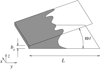
FIG. 1.: Schismatic representation of the Helle-Shaw cell with lifting plates, showing the parameters used in the text.

It should be here noted that mass (and density) conservation requires that, neither bubbles are formed nor drops of the displaced fluid are left behind during the lifting process. This condition, although unlikely accomplished in actual experiments, it is probably unavoidable in analytical calculations. Eq. (5), combined with the Poiseuille-Darcy equation (Eq. (3)), gives the differential equation (growth law) which governs flow in the HS cell with lifting plates,

$$\nabla^{2}P_{j}+\frac{3a}{b}\frac{\partial P_{j}}{\partial y}=\frac{12\mu_{j}\dot{a}y}{b^{3}}\;,$$ (6)

where $\dot{a}$ expresses the derivative of $a$ with respect to time. It is interesting to note that this is an inhomogeneous equation as opposed to the homogeneous one reported in Ref. [4]. The inhomogeneous term comes from the time dependence of the gap (Eq. (4)) and it is not present in the growth law for the HS with a gap gradient, as already found by Zhao et al[4, 8]. Note, however, that the inhomogeneous term is essential in this case, as no fluid is injected at the open end of the cell to promote fluid motion (see below). We also note that including the spatial dependence of the gap $b$ in Eq. (5) leads lo a factor 3 in the second term of Eq. (6), as opposed to the factor 2 reported in Ref. [4] and in agreement with Zhao et al[8]. This change in the growth law makes calculations slightly more complicated. As regards the comparison with the directional solidification problem, we note that Eq. (6) is similar to that which describes directional solidification in some unsteady-state[7].

In discussing the boundary conditions let $L$ be the length of the cell and $L_{i}$ the length of the zone occupied by the more viscous fluid at $t$=0. On the other hand, and in order to carry out the linear stability analysis, we assume that the interface between the two fluids, instead of being flat, is slightly perturbed as $y_{p}=y_{i}+\delta{\rm e}^{iqx}$, where $\delta=\delta_{0}{\rm e}^{\gamma t}$ is the time–dependent amplitude of the perturbation (assumed to be much smaller than $y_{i}$) and $q$ its wavenumber.

The first boundary condition accounts for the fact that the fixed end of the cell ($y=0$) is closed,

$$v_{1y}(0)=0\;.$$ (7)

On the other hand, the velocities of the two fluids must be equal at the interface

$$v_{1y}(y_{p})=v_{2y}(y_{p})\;.$$ (8)

Finally the forces which the fluids exert on each other at the common interface must be equal and opposite. This condition can be approximated by

$$P_{1}(y_{p})-P_{2}(y_{p})=\sigma\left[\frac{1}{R_{x}(y_{p})}+\frac{1}{R_{z}(y_{p})}\right]\;,$$ (9)

where $\sigma$ is the surface-tension (the interfacial tension associated to the interface between the two fluids) and $R_{x}$, $R_{z}$, the principle radii of curvature of the interface at a given point,

$$\frac{1}{R_{x}(y_{p})}=-\frac{\partial^{2}y_{p}}{\partial x^{2}}\;,$$ (11)

$$\frac{1}{R_{z}(y_{p})}\approx\frac{1}{b(y_{i},t)}\;.$$ (12)

The latter equation is related to wetting effects. Although, as already reported by other authors[8, 12, 13], we have found that these effects give a negligible contribution, we have kept this term all throughout the calculation.

III linear stability analysis

Once the plane interface is perturbed, the most general solution of Eq.(6) can be written as

$$P_{j}(x,y)=f_{j}(y)+g_{j}(y)e^{iqx}\;,$$ (13)

where $g_{j}(y)$ is proportional to the amplitude of the perturbation $\delta$. Introducing Eq. (11) into the growth law (Eq. (6)) we obtain,

$$\frac{\partial^{2}f_{j}}{\partial y^{2}}+\frac{3a}{b}\frac{\partial f_{j}}{\partial y}=\frac{12\mu_{j}\dot{a}y}{b^{3}}\;,$$ (15)

$$\frac{\partial^{2}g_{j}}{\partial y^{2}}+\frac{3a}{b}\frac{\partial g_{j}}{\partial y}-q^{2}g_{j}=0\;.$$ (16)

The boundary conditions for the fluid velocity at the closed end give

$$\left.\frac{\partial f_{1}}{\partial y}\right|_{y=0}=0\;,$$ (18)

$$\left.\frac{\partial g_{1}}{\partial y}\right|_{y=0}=0\;.$$ (19)

Note that in order to obtain physically meaningful solutions we should also require that the perturbation be damped in the open end of the cell, this means that $(\partial g_{2}/\partial y)|_{y=L}=0$. This assumption will be valid whenever the viscosity $\mu_{2}$ is very small (note that, in the present work, we will analyze experiments in which fluid 2 is air). The continuity of the velocity at the interface between the two fluids leads to (up to first order in $\delta$):

$$\frac{1}{\mu_{1}}\left.\frac{\partial f_{1}}{\partial y}\right|_{y=y_{i}}=\frac{1}{\mu_{2}}\left.\frac{\partial f_{2}}{\partial y}\right|_{y=y_{i}}\;,$$ (21)

$$\frac{1}{\mu_{1}}\left(\left.\delta\frac{\partial^{2}f_{1}}{\partial y^{2}}+\frac{\partial g_{1}}{\partial y}\right)\right|_{y=y_{i}}\!\!\!\!\!\!=\frac{1}{\mu_{2}}\left.\left(\delta\frac{\partial^{2}f_{2}}{\partial y^{2}}+\frac{\partial g_{2}}{\partial y}\right)\right|_{y=y_{i}}\!\!\!\!\!\!\!.$$ (22)

Finally, the continuity of forces at the interface gives

$$\left[f_{1}-f_{2}-\frac{\sigma}{R_{z}}\right]_{y=y_{i}}=0\;,$$ (24)

$$\left[g_{1}-g_{2}(y)\right]_{y=y_{i}}\!\!\!=-\left[\frac{\partial\left(f_{1}-f_{2}\right)}{\partial y}\right]_{y=y_{i}}\!\!\!-\sigma q^{2}\;.$$ (25)

The solution of Eq. (12a), using the boundary conditions Eqs. (13a) and (14a) can be written as,

$$f_{j}=\frac{12\mu_{j}\dot{a}}{a^{3}}\!\left(\frac{b_{0}}{b(y,t)}\!+\!\frac{1}{2}\ln b(y,t)\!-\!\frac{b_{0}^{2}}{4b(y,t)^{2}}\right)\!+\!A_{j},$$ (26)

where $A_{j}$ ($j$=1,2) are constants that can be determined from the boundary condition of Eq. (15a) (we will not need them here). It should be noted that, had Eq. (6) been homogeneous, the solution of Eq. (12a) would have been, $f_{j}=A_{j}-B_{j}/b(y,t)^{2}$, which, after proper use of the boundary conditions, gives a uniform pressure field and, therefore, no fluid motion, as remarked above. On the other hand the solution of Eq. (12b) is

$$g_{j}=\frac{1}{\xi}\left[C_{j}I_{1}(\xi)+D_{j}K_{1}(\xi)\right]\;,\hskip 28.45274ptj=1,2\;,$$ (27)

and its derivative,

$$\frac{\partial g_{j}}{\partial y}=\frac{q}{\xi}\left[C_{j}I_{2}(\xi)-D_{j}K_{2}(\xi)\right]\;,\hskip 28.45274ptj=1,2\;,$$ (28)

where $\xi=qb(y,t)/a$, and $I_{1}(\xi)$, $I_{2}(\xi)$, and $K_{1}(\xi)$, $K_{2}(\xi)$ are the first and the second order modified Bessel functions. The constants $C_{j}$, $D_{j}$ have to be determined from the boundary conditions,

$$C_{1}I_{2}(\xi_{0})-D_{1}K_{2}(\xi_{0})=0\;,$$ (30)

$$C_{2}I_{2}(\xi_{L})-D_{2}K_{2}(\xi_{L})=0\;,$$ (31)

$$\left(\frac{C_{1}}{\mu_{1}}-\frac{C_{2}}{\mu_{2}}\right)I_{2}({\xi_{i}})-\left(\frac{D_{1}}{\mu_{1}}-\frac{D_{2}}{\mu_{2}}\right)K_{2}({\xi_{i}})=0\;,$$ (32)

$$(C_{1}-C_{2})I_{1}(\xi_{i})+(D_{1}-D_{2})K_{1}(\xi_{i})=\epsilon\delta\;,$$ (33)

where $\xi_{0}=qb_{0}/a$, $\xi_{i}=q(b_{0}+ay_{i})/a$, $\xi_{L}=q(b_{0}+aL)/a$, and $\epsilon$ is given by,

$$\epsilon=\xi_{i}\left[\frac{12(\mu_{1}-\mu_{2})V_{i}(y_{i})}{b(y_{i},t)^{2}}+\sigma q^{2}\right]\;,$$ (34)

where the velocity of the interface between the two fluids is given by,

$$V_{i}(t)=-\frac{b^{2}}{12\mu_{j}}\left.\frac{\partial f_{j}}{\partial y}\right|_{y=y_{i}}\!\!\!={\dot{y}}_{i}=-\frac{{\dot{a}}y_{i}^{2}}{2b(y_{i},t)}\;,$$ (35)

independent of $j$. Note that, due to the choice of the origin of coordinates, this velocity is negative. Integrating this velocity gives an expression for the position of the interface (where the boundary $y(t=0)=L_{i}$ is taken):

$$y_{i}(t)=\frac{\sqrt{b_{0}^{2}+2L_{i}b_{0}a}-b_{0}}{a}\;.$$ (36)

which is the same result as if we had considered the simpler mass conservation as $\frac{1}{2}ay_{i}^{2}+b_{0}y_{i}=b_{0}L$.

Now, we have all the ingredients to calculate the instantaneous velocity of the interface (growth rate), which can be calculated from the Poiseuille-Darcy equation. The result is,

$$v_{1y}(y_{p}) = \dot{y_{p}}=\dot{y_{i}}+\dot{\delta}{\rm e}^{iqx}$$ (37)

$$= -\frac{b}{12\mu_{1}}\left.\frac{\partial(f_{1}+g_{1}{\rm e}^{iqx})}{\partial y}\right|_{y=y_{p}}\;.$$ (38)

From which we obtain the velocity of the perturbation $\gamma$,

$$\gamma=\frac{\dot{\delta}}{\delta}=-\frac{\dot{b}(y_{i},t)}{b(y_{i},t)}-\frac{ab(y_{i},t)\epsilon}{12}Z(\xi_{i},\xi_{L})\;,$$ (39)

where,

$$Z(\xi_{i},\xi_{r})=\frac{I_{2}(\xi_{i})}{I_{1}(\xi_{i})} \times \left(\mu_{1}\frac{\left[G_{2}(\xi_{0})+G_{1}(\xi_{i})\right]}{\left[G_{2}(\xi_{0})-G_{2}(\xi_{i})\right]}\right.$$ (41)

$$\left.-\mu_{2}\frac{\left[G_{2}(\xi_{L})+G_{1}(\xi_{i})\right]}{\left[G_{2}(\xi_{L})-G_{2}(\xi_{i})\right]}\right)^{-1}\!\!\!,$$

and,

$$G_{j}(\xi)=K_{j}(\xi)/I_{j}(\xi)\;,\hskip 28.45274ptj=1,2\;.$$ (42)

At the very beginning of liftting $1<<\xi_{0}\lesssim\xi_{i}\lesssim\xi_{L}$. As a consequence, $G_{1}(\xi_{i})\simeq G_{2}(\xi_{i})$. On the other hand, and due to the exponential behavior of the Bessel and Hankel functions, $G_{2}(\xi_{0})>>G_{2}(\xi_{i})>>G_{2}(\xi_{L})$. Thus, Eq. (23b) can be approximated as

$$\gamma = -\frac{\dot{b}(y_{i},t)}{b(y_{i},t)}$$ (44)

$$-\frac{b(y_{i},t)^{2}}{\mu_{1}+\mu_{2}}q\left[\frac{12(\mu_{1}-\mu_{2})V_{i}(t)}{b(y_{i},t)^{2}}+\sigma q^{2}\right]\;.$$

The wavenumber of the dominant mode $q_{d}$ results to be,

$$q_{d}^{2}=\frac{4(\mu_{1}-\mu_{2})V_{i}(t)}{\sigma b(y_{i},t)^{2}}\;.$$ (45)

This result is quite similar to that obtained for the standard Hele-Shaw cell. The only difference resides upon the fact that the interface velocity $V_{i}(t)$ and the gap $b(y_{i},t)$ now depend on time. As regards the cutoff wavenumber, we note that if the first term in the r.h.s of Eq. (27) is neglected (in fact it is quite small for most of the experimental configurations and conditions), the result is again equivalent to that of the standard cell ($q_{c}^{2}=3q_{d}^{2}$). If it is not neglected, a minimum wavenumber, below which the system is stable, is also found.

At $t=0$, the dominant mode is

$$q_{d}^{2}=\frac{4(\mu_{1}-\mu_{2})}{\sigma b_{0}^{2}}V_{i}(0)\;,$$ (46)

where $V_{i}(0)$ is the velocity of the interface at $t=0$,

$$V_{i}(0)=\frac{\omega L_{i}^{2}}{2b_{0}}\;.$$ (47)

$V_{i}(0)$ introduces a dependence on the cell parameters of the wavenumber of the dominant mode, not present in the standard cell. In particular, $q_{d}$ depends on the square of the length occupied by the displaced (more viscous) fluid. It is also inversely proportional to the gap, leading to a $b_{0}^{-3}$ dependence of $q_{d}$, as opposed to $b_{0}^{-2}$ in the standard cell. These differences could be easily checked experimentally.

IV Numerical Results and Discussion

At the beginning of lifting ($t=0$) the process is governed by Eq. (30). In actual experiments, as the less viscous fluid is commonly air, $\mu_{2}\approx 0$, and the wavelength of the dominant and the cutoff modes are given by expressions identical to those for the standard cell, namely, $\lambda_{d}/b_{0}=\pi(\sigma/\mu_{1}V_{i}(0))^{1/2}$, and $\lambda_{c}=\lambda_{d}/\sqrt{3}$, respectively. In order to estimate the wavelength of the dominant mode we consider the experimental set up investigated by Zhao et al [8]. These authors used air/glycerine ($\mu$ = 65 mPa and $\sigma$=29.5 N/m) in a cell with a gap of 2.5 mm and a length of 1 m (we assume that glycerine fills the whole cell). Taking $\omega$ = 0.001 rad/s, $\lambda_{d}\approx$ 1.2 cm. This result decreases in an order of magnitude if, as done by Ben–Jacob et al [5], the lifting rate is increased in two orders of magnitude. We cannot precisely compare our results with the data obtained by the latter authors as they do not give important parameters such as the length and gap of the cell.

FIG. 2.: Results for the velocity of the perturbation $\gamma$ (rad/s) as a function of its wavenumber $q$ (cm^-1), for several times after lifting is initiated: $t$=0 s (continuous line), $t$=0.5 s (chain line) and $t$=1 s (dashed line) . The results correspond to the cell parameters of Ref. [7], namely: air/glycerine ($\mu$ = 65 mPa and $\sigma$=29.5 N/m) in a cell with a gap of 2.5 mm and a length of 1 m (we assume that glycerine fills the whole cell). The lifting rate is $\omega$ = 0.001 rad/s.

If instead of glycerine we consider water, at $t=0$ and for the same cell parameters, the wavelength of the dominant mode results to be $\approx$ 0.4 cm^-1, which leads to a wavelength of $\approx$ 16 cm. This wavelength is of the order of the full width of standard cells and therefore one should not expect the formation of fingers. Further we note that the velocity of the perturbation results to be at least an order of magnitude smaller than for glycerine, reinforcing our view that the flat front would be rather stable. Note that this result is also obtained for the standard cell and that it is in agreement with the experimental observations. The only way to increase the tendency towards instabilities would be to increase the velocity of the interface which in the present case can be accomplished by increasing $L$ and the lifting rate and/or decreasing $b_{0}$.

As lifting proceeds, fingers are being formed and a linear stability analysis such as that carried out here is no longer strictly valid. However, some information valid to understand specific features of the growing process may be obtained from the results of a linear stability analysis, as already found in the case of growth in systems governed by Poisson’s equation [10]. In Figure 2 we report our results for the velocity at which the perturbation propagates as a function of the perturbation wavenumber, for several times after lifting was initiated. In the calculations the first term in the r.h.s. of Eq. (27) was neglected. The results correspond to the cell parameters given in the preceeding paragraph and a lifting rate of $\omega$=0.001 rad/s. It is noted that the velocity of the perturbation $\gamma$ strongly decreases with time. In fact the value at its maximum is reduced in more than a factor of 5 after lifting the cell for 1 second. The wavanumber at which $\gamma$ shows a maximum (dominant mode) and cutoff wavenumber do also decrease with time (see Fig. 3). The decrease of the velocity of propagation of the perturbation suggest a lower tendency towards instabilities and, thus, a larger fractal dimension of the aggregates (this is compatible with a decreasing $q_{d}$). A variation in the fractal dimension of the aggregates as growth (lifting) proceeds was also found by Roche et al [9] in their simulations of the Poisson equation, which they argue to be adequate for the HS with lifting plates (note that this is approximately correct if the term proportional to the first derivative of the pressure in Eq. (6) is either neglected or replaced by a constant). However they found that the simulation which seemed to describe more closely the experimental situation gave an increasing fractal dimension.

FIG. 3.: Wavenumbers (cm^-1) of the dominant ($q_{d}$, continuous line) and cutoff ($q_{c}$, broken line) modes as a function of time (s) in the Hele–Shaw with lifting plates investigated in this work. The results correspond to the parameters given in the caption of Fig. 1.

Summarizing, we have presented a linear stability study of the HS with lifting plates. We have first derived the basic equations which result to be that of the directional solidification problem under some unsteady conditions. Despite the simplifications made to do the analytical work (we do not treat completely the wetting effects and neglect the fluid that stays attached to the plates), the results for the wavelength of the dominant mode seem to be compatible with the available experimental data. It will be worth carrying out more experiments in order to get more information on the dependence of the characteristics of the growing aggregates on the parameters of the cell.

- [1] Present address: Physics Department, Liaoming University, Shenyang, 110036 P.R. China.
- [2] P.G. Saffman and G.I. Taylor, Proc. R. Soc. Lond. 245, 312 (1958).
- [3] D.C. Hong and J.S. Langer, Phys. Rev. Lett. 56, 2032 (1986); J.V. Maher, ibid.54, 1498 (1985); B.I. Schraiman, ibid.56, 2028 (1985).
- [4] K.V. Cloud and J.V. Maher, Physics Reports 260, 139 (1995).
- [5] E. Ben-Jacob, R. Godbey, N.D. Goldenfeld, H. Levine, T. Mueller and L.M. Sander, Phys. Rev. Lett. 55, 1315 (1985).
- [6] J.S. Langer, Rev. Mod. Phys. 52, 1 (1980).
- [7] W. Kurz and D.J. Fisher, Fundamentals of Solidification (Trans Tech Publications, Switzerland, 1989).
- [8] H. Zhao, J. Casademunt, C. Yeung and J.V. Maher, Phys. Rev. A 45, 2455 (1992).
- [9] H. La Roche, J.F. Fernández, M. Octavio, A.G. Loeser and C.J. Lobb, Phys. Rev. A 44, R6185 (1991).
- [10] E. Louis, O. Pla, L.M. Sander and F. Guinea, Modern Phys. Lett. B 8, 1739 (1994).
- [11] L.D. Landau and E.M. Lifshitz, Fluid Mechanics (Pergamon Press, New York, 1987).
- [12] D. Bensimon, L.P. Kadanoff, S. Liang, B.I. Schraiman and C.Tang, Rev. Mod. Phys. 58, 977 (1986).
- [13] C.-W. Park and G.M. Homsy, J. Fluid Mech. 139, 291 (1984).