The asymptotic behaviour
of the initially separated
A $+$ B(static) $\to$ 0 reaction-diffusion systems

Abstract

We examine the long-time behaviour of A $+$ B(static) $\to$ 0 reaction-diffusion systems with initially separated species A and B. All of our analysis is carried out for arbitrary (positive) values of the diffusion constant $D_{\mathrm{A}}$ of particles A and initial concentrations $a_{0}$ and $b_{0}$ of A’s and B’s. We derive general formulae for the location of the reaction zone centre, the total reaction rate, and the concentration profile of species A outside the reaction zone. The general properties of the reaction zone are studied with a help of the scaling ansatz. Using the mean-field approximation we find the functional forms of ‘tails’ of the reaction rate $R$ and the dependence of the width of the reaction zone on the external parameters of the system. We also study the change in the kinetics of the system with $D_{\mathrm{B}}>0$ in the limit $D_{\mathrm{B}}\to 0$. Our results are supported by numerical solutions of the mean-field reaction-diffusion equation.

1 Introduction

Investigation of the reaction fronts formed in the reaction-diffusion processes of the type A $+$ B $\to$ 0 with initially separated species A and B has attracted a lot of recent interest. This is due to the fact that not only the kinetics of such systems exhibits many surprising features [1, 2, 3, 4, 5], but they are also amenable to experimental studies [3, 6, 7].

A standard way to treat the initially separated problem analytically is to solve the partial differential equations [1]

$$\begin{array}[]{rcl}\frac{\textstyle\partial{\rho_{\mathrm{A}}}}{\textstyle\partial t}&=&D_{\mathrm{A}}\frac{\textstyle\partial^{2}{\rho_{\mathrm{A}}}}{\textstyle\partial x^{2}}-R\,,\\[8.61108pt] \frac{\textstyle\partial{\rho_{\mathrm{B}}}}{\textstyle\partial t}&=&D_{\mathrm{B}}\frac{\textstyle\partial^{2}{\rho_{\mathrm{B}}}}{\textstyle\partial x^{2}}-R\,,\end{array}$$ (1)

with the initial state given by

$$\begin{array}[]{rcl}\rho_{\mathrm{A}}(x,t=0)&=&a_{0}H(-x)\,,\\[4.30554pt] \rho_{\mathrm{B}}(x,t=0)&=&b_{0}H(x)\,,\end{array}$$ (2)

where $\rho_{\mathrm{A}}(x,t)$ and $\rho_{\mathrm{B}}(x,t)$ are the mean local concentrations of A’s and B’s, $R$ is the macroscopic reaction rate, $H(x)$ denotes the Heavyside step function, and $a_{0}$, $b_{0}$, $D_{\mathrm{A}}$ and $D_{\mathrm{B}}$ are some constants related to the initial concentrations of species A and B and their diffusion coefficients, respectively.

Equations (1) present the macroscopic approach to the problem. However, it has not been established yet how to relate the macroscopic reaction rate $R$ to the microscopic picture of the initially separated reaction-diffusion systems below or at the critical dimension $d_{\mathrm{c}}=2$. Dimensional [8, 9, 10] and renormalisation group analyses [11, 12, 13] lead to the conclusion that above $d_{\mathrm{c}}$ one can adopt the mean-field approximation $R=k\rho_{\mathrm{A}}\rho_{\mathrm{B}}$, with $k$ being a constant. For 2D systems one expects logarithmic corrections to the mean-field picture [9, 10, 13]. One dimensional systems are usually studied by examining microscopic models in which, upon contact, the members of a pair A–B react with some probability $p$ [10, 11, 12, 13, 14, 15, 16, 17, 18]. The analytical form of $R(x,t)$ was derived for $D_{\mathrm{B}}=0$ [14], and for $D_{\mathrm{B}}>0$ and $|x|\to\infty$ [12].

There are, however, several techniques which enables one to derive a lot of useful information from (1) even for $d\leq d_{\mathrm{c}}$, i.e. when the explicit form of $R$ remains unknown. They are concentrated on the asymptotic, long-time behaviour of the reaction-diffusion systems, and include the renormalisation group analysis [11, 12, 13, 17], the scaling ansatz [1, 10], the quasistationary approximation [8, 19], and our approach of Ref. [20].

According to the scaling ansatz [1], the long-time behaviour of the reaction-diffusion system inside the reaction layer can be described with a help of some scaling functions $S_{\mathrm{A}}$, $S_{\mathrm{B}}$ and $S_{\mathrm{R}}$ through

$$\rho_{\mathrm{A}}(x,t) = \eta_{\mathrm{A}}t^{-\gamma_{\mathrm{A}}}S_{\mathrm{A}}\!\left(x-x_{\mathrm{f}}(t)\over w(t)\right)\,,$$ (3)

$$\rho_{\mathrm{B}}(x,t) = \eta_{\mathrm{B}}t^{-\gamma_{\mathrm{B}}}S_{\mathrm{B}}\!\left(x-x_{\mathrm{f}}(t)\over w(t)\right)\,,$$ (4)

$$R(x,t) = \eta_{\mathrm{R}}t^{-\beta}S_{\mathrm{R}}\!\left(x-x_{\mathrm{f}}(t)\over w(t)\right)\,,$$ (5)

where $x_{\mathrm{f}}(t)\propto t^{1/2}$ denotes the point at which the reaction rate $R$ attains its maximal value, $w(t)\propto t^{\alpha}\ll t^{1/2}$ is the width of the reaction zone, $\eta_{\mathrm{A}}$, $\eta_{\mathrm{B}}$ and $\eta_{\mathrm{R}}$ are some parameters independent of $x$ and $t$, and exponents $\alpha$, $\beta$, $\gamma_{\mathrm{A}}$ and $\gamma_{\mathrm{B}}$ are some positive constants given, for $R\propto\rho_{\mathrm{A}}\rho_{\mathrm{B}}$ and nonzero diffusion constants, by $\alpha=\frac{1}{6}$, $\beta=\frac{2}{3}$ and $\gamma_{\mathrm{A}}=\gamma_{\mathrm{B}}=\frac{1}{3}$.

The quasistationary approximation [8, 19] consists in the assumption that at sufficiently long times the kinetics of the front is governed by two characteristic time scales. One of them, $\tau_{\mathrm{J}}\propto(\!{\d}\log\!J/\!{\d}t)^{-1}\propto t$, controls the rate of change in the diffusive current $J$ of particles arriving at the reaction layer. The other one, $\tau_{\mathrm{F}}\propto w^{2}\propto t^{2\alpha}$, is the equilibration time of the reaction front. If $\alpha<1/2$ then $\tau_{\mathrm{F}}/\tau_{\mathrm{J}}\to 0$ as $t\to\infty$. Therefore, as $t\to\infty$, in the vicinity of $x_{\mathrm{f}}$ the left sides of (1) become negligibly small compared to other terms. Consequently, if $D_{\mathrm{A}}$ and $D_{\mathrm{B}}$ are both nonzero, the asymptotic form of $\rho_{\mathrm{A}}$ and $\rho_{\mathrm{B}}$ inside the reaction layer is governed by much simpler equations

$$\begin{array}[]{rcl}D_{\mathrm{A}}\frac{\textstyle\partial^{2}{\rho_{\mathrm{A}}}}{\textstyle\partial x^{2}}&=&R\,,\\[8.61108pt] D_{\mathrm{B}}\frac{\textstyle\partial^{2}{\rho_{\mathrm{B}}}}{\textstyle\partial x^{2}}&=&R\,,\end{array}$$ (6)

which are to be solved with the boundary conditions

$$\begin{array}[]{rcl}\partial\rho_{\mathrm{A}}/\partial x\to-J_{\mathrm{A}}(t),\;\rho_{\mathrm{B}}\to 0&\;\mbox{as}&x\to-\infty\,,\\[4.30554pt] \partial\rho_{\mathrm{B}}/\partial x\to J_{\mathrm{B}}(t),\;\rho_{\mathrm{A}}\to 0&\;\mbox{as}&x\to+\infty\,.\end{array}$$ (7)

The most important feature of the quasistationary equations (6) is that they depend only on $x$, with time $t$ being a parameter entering their solutions $\rho_{\mathrm{A}}(x,t)$ and $\rho_{\mathrm{B}}(x,t)$ only through the time dependent boundary currents $J_{\mathrm{A}}=J_{\mathrm{B}}$ whose dependence on $t$, $D_{\mathrm{A}}$, $D_{\mathrm{B}}$, $a_{0}$ and $b_{0}$ has recently been derived analytically [20].

In a recent paper [20] we employed the quasistatic approximation to develop a new method of investigating the asymptotic kinetics of the initially separated reaction-diffusion systems. A peculiar feature of that approach is that it is concentrated mainly on the properties of the system outside the reaction zone. In this way, without imposing any special restrictions on the form of $R$, it relates exactly many quantities of physical interest to the values of external parameters $a_{0}$, $b_{0}$, $D_{\mathrm{A}}$ and $D_{\mathrm{B}}$, which will enable us to investigate the limit $D_{\mathrm{B}}\to 0$ analytically. In particular it was shown that there exist two limits, $C_{\mathrm{f}}=\lim_{t\to\infty}x_{\mathrm{f}}(t)/\sqrt{t}$ and $C_{\mathrm{J}}=\lim_{t\to\infty}J(t)\sqrt{t}$. Given $a_{0}$, $b_{0}$, $D_{\mathrm{A}}$ and $D_{\mathrm{B}}$, the value of $C_{\mathrm{f}}$ can by computed by solving

$$\Phi\!\left(\frac{-C_{\mathrm{f}}}{2\sqrt{D_{\mathrm{A}}}}\right)=\frac{a_{0}\sqrt{D_{\mathrm{A}}}}{b_{0}\sqrt{D_{\mathrm{B}}}}\>\Phi\!\left(\frac{C_{\mathrm{f}}}{2\sqrt{D_{\mathrm{B}}}}\right)\,,$$ (8)

where

$$\Phi(x)\equiv\!\left[1-\>\!\mbox{erf}\!\left(x\right)\right]\exp(x^{2})\,,$$ (9)

and $\;\>\!\mbox{erf}\!\left(x\right)\equiv 2\pi^{-1/2}\!\int_{0}^{x}\exp(-\eta^{2}){\d}\eta\;$ is the error function [21]. Then $C_{\mathrm{J}}$ can be calculated by solving

$$C_{\mathrm{f}}=2\sqrt{D_{\mathrm{A}}}\>\!\mbox{erf${}^{-1}$}\left[(a_{0}-C_{\mathrm{A}})/C_{\mathrm{A}}\right]=2\sqrt{D_{\mathrm{B}}}\>\!\mbox{erf${}^{-1}$}\left[(C_{\mathrm{B}}-b_{0})/C_{\mathrm{B}}\right]$$ (10)

and

$$C_{\mathrm{J}}=C_{\mathrm{A}}\sqrt{D_{\mathrm{A}}\over\pi}\exp\!\!\left(-\frac{C_{\mathrm{f}}^{2}}{4D_{\mathrm{A}}}\right)=C_{\mathrm{B}}\sqrt{D_{\mathrm{B}}\over\pi}\exp\!\!\left(-\frac{C_{\mathrm{f}}^{2}}{4D_{\mathrm{B}}}\right)\,,$$ (11)

where $C_{\mathrm{A}}$ and $C_{\mathrm{B}}$ are some constants controlling the form of $\rho_{\mathrm{A}}$ and $\rho_{\mathrm{B}}$ outside the reaction zone; specifically, for $x\ll x_{\mathrm{f}}-w$ we have

$$\rho_{\mathrm{A}}(x,t)=a_{0}-C_{\mathrm{A}}\!\left[\>\!\mbox{erf}\!\left(x/\!\sqrt{4D_{\mathrm{A}}t}\right)+1\right]\,,$$ (12)

and for $x\gg x_{\mathrm{f}}+w$ there is

$$\rho_{\mathrm{B}}(x,t)=b_{0}+C_{\mathrm{B}}\!\left[\>\!\mbox{erf}\!\left(x/\!\sqrt{4D_{\mathrm{B}}t}\right)-1\right]\,.$$ (13)

It was confirmed by several methods, including the renormalisation group analysis [11, 12], numerical simulations [22] and heuristic arguments [20], that the values of the exponents $\alpha$, $\beta$, $\gamma_{\mathrm{A}}$ and $\gamma_{\mathrm{B}}$ as well as the form of the scaling functions $S_{\mathrm{A}}$, $S_{\mathrm{B}}$ and $S_{\mathrm{R}}$ do not depend on $D_{\mathrm{A}}$, $D_{\mathrm{B}}$, $a_{0}$ and $b_{0}$ if the values of these parameters are nonzero. However, when one of the components is immobile (or ‘static’), the asymptotic kinetics of the reaction front can change dramatically. For example, in the mean-field approximation the width of the front converges to a stationary value, and the reaction rate at $x_{\mathrm{f}}$ decreases as $t^{-1/2}$, which corresponds to $\alpha=0$ and $\beta=\frac{1}{2}$ [4, 22]. We have therefore two asymptotic universality classes: one characteristic for the ‘dynamic’ systems in which both components diffuse, and the ‘quasistatic’ one observed if one of the diffusion constants is zero. Henceforth we shall assume $D_{\mathrm{A}}>0$, so the two asymptotic universality classes will be distinguished by determining whether $D_{\mathrm{B}}=0$ or $D_{\mathrm{B}}>0$.

Although the peculiar kinetics of the systems with $D_{\mathrm{B}}=0$ was noticed quite early, so far nearly all of the research has been concentrated on the systems in which both of the diffusion constants $D_{\mathrm{A}}$ and $D_{\mathrm{B}}$ are nonzero. Closer inspection of the powerful methods developed in the last decade to investigate the reaction-diffusion systems reveals that only the scaling ansatz, which is a purely mathematical concept, can be trivially employed to investigate both kinds of the systems. However, since even this relatively simple approach has so far been carried out only for the ‘dynamic’ problem [1, 10], the theories of the two asymptotic universality classes remain practically disconnected.

Several factors have lead to this situation. Theoretical results [14] derived for the case $D_{\mathrm{B}}=0$ utilized the basic property of such systems, immobility of particles B, in a way that cannot be extended for systems with $D_{\mathrm{B}}>0$. On the other hand, most of the fundamental techniques developed for the case $D_{\mathrm{B}}>0$ has been based on the quasistationary approximation which requires that the ratio $J_{\mathrm{A}}/J_{\mathrm{B}}$ of two opposite currents of particles A and B entering the reaction zone should asymptotically go to 1. This condition cannot be met by the systems with $D_{\mathrm{B}}=0$, as in this case $J_{\mathrm{B}}(t)\equiv 0$.

The aim of our paper is to unify our understanding of these two kinds of the reaction-diffusion systems. The procedure we are using consists in detailed examination of the case $D_{\mathrm{B}}=0$ and comparison of the results with those already derived for $D_{\mathrm{B}}>0$. We study the systems with $D_{\mathrm{B}}=0$ by means of various methods and for arbitrary (positive) values of $a_{0}$, $b_{0}$, and $D_{\mathrm{A}}$. In particular we show the counterpart of the quasistationary approximation (6) which should be used if $D_{\mathrm{B}}=0$. We argue that the form of these equations, as well as their boundary conditions, determine the properties of the asymptotic universality classes. In subsequent sections we study these properties for the systems with $D_{\mathrm{B}}=0$ using the heuristic theory of Ref. [20], the scaling ansatz, the mean-field approximation, and numerical analysis. Although some aspects of the systems with $D_{\mathrm{B}}=0$ turn out to be the same as of those with $D_{\mathrm{B}}>0$, our analysis implies that these two cases should always be considered separately.

2 The limit $D_{\mathrm{B}}\to 0$

Consider equations (8) – (13) with the values of $D_{\mathrm{A}}$, $a_{0}$ and $b_{0}$ fixed at some positive values, and $D_{\mathrm{B}}$ going to 0. For physical reasons we expect that as $D_{\mathrm{B}}$ goes to 0, $C_{\mathrm{f}}$ converges to some nonzero limiting value, and so the argument of $\Phi$ on the right hand side of (8) diverges to infinity. We can therefore use an asymptotic property of the error function, $x(1-\>\!\mbox{erf}\!\left(x\right))\exp(x^{2})\to 1/\sqrt{\pi}$ as $x\to\infty$ [21], and reduce (8) to

$$\Phi\!\left(\frac{-C_{\mathrm{f}}}{2\sqrt{D_{\mathrm{A}}}}\right)=\frac{2a_{0}\sqrt{D_{\mathrm{A}}}}{\sqrt{\pi}b_{0}C_{\mathrm{f}}}\,.$$ (14)

Since $\Phi(x)$ diminishes monotonically from $\infty$ to $0$ as $x$ grows from $-\infty$ to $\infty$, the above equation has a unique, positive solution. Consequently, (10) and (11) imply that $C_{\mathrm{J}}$ and $C_{\mathrm{A}}$ also converge to some positive values, but $C_{\mathrm{B}}$ rapidly diverges to infinity.

One can now use (10), (11) and (14) to arrive, after some algebra, at an important relation valid only if $D_{\mathrm{B}}=0$

$$b_{0}C_{\mathrm{f}}=2C_{\mathrm{J}}\,.$$ (15)

This equation has a very natural physical interpretation. On the one hand the total number $M(t)$ of reactions occurring by time $t$ is asymptotically equal

$$\int_{0}^{t}\!J_{\mathrm{A}}(\tau){\d}\tau\,\sim\,\int_{0}^{t}\!C_{\mathrm{J}}/\sqrt{\tau}{\d}\tau\,\sim\,2C_{\mathrm{J}}\sqrt{t}\,.$$ (16)

On the other hand, however, for $x\gg x_{\mathrm{f}}+w$ we have $\rho_{\mathrm{B}}\sim b_{0}$, and for $x\ll x_{\mathrm{f}}-w$ we expect $\rho_{\mathrm{B}}\sim 0$. Neglecting terms of order $b_{0}w\ll b_{0}t^{1/2}$ we thus conclude that $M(t)$ can as well be estimated by

$$\int_{-\infty}^{\infty}[\rho_{\mathrm{B}}(x,t)-\rho_{\mathrm{B}}(x,0)]{\d}x\,\sim\,b_{0}x_{\mathrm{f}}(t)\,\sim\,b_{0}C_{\mathrm{f}}\sqrt{t}\,,$$ (17)

which leads to (15).

Our theory is consistent with the numerical simulations of Larralde et al [14], who considered the one dimensional system (i.e. for $d<d_{\mathrm{c}}$) with $D_{\mathrm{B}}=0$, $D_{\mathrm{A}}=1/2$ and $a_{0}/b_{0}=1$. They found that, respectively, for $t=500$, 1000 and 5000 the value of $x_{\mathrm{f}}(t)$ was approximately equal to $11\pm 0.5$, $16\pm 0.5$ and $36\pm 0.5$, so that $x_{\mathrm{f}}/\sqrt{t}\approx$ $0.492\pm 0.022$, $0.506\pm 0.016$ and $0.509\pm 0.07$, respectively. This is in excellent agreement with our equation (14), whose numerical solution reads $C_{\mathrm{f}}\approx 0.5060$. Below, in Section 5, we will also verify our theory using the mean-field approximation (i.e. for $d>d_{\mathrm{c}}$).

3 General consequences of the scaling ansatz

Let $D_{\mathrm{B}}=0$ and $D_{\mathrm{A}}$, $a_{0}$ and $b_{0}$ take on arbitrary (positive) values. Assume that the asymptotic solutions of the Gálfi and Rácz problem (1) in the long-time limit take on the scaling form (3) – (5) with $\alpha<1/2$. Inserting (3) and (4) into (1) and taking the limit $t\to\infty$ we find that at any $x$ such that $|x-x_{\mathrm{f}}|\ll t^{1/2}$ there is

$$\frac{\textstyle\partial{\rho_{\mathrm{A}}}}{\textstyle\partial t}\,\propto\,t^{-\gamma_{\mathrm{A}}-\alpha-1/2}\quad\mbox{and}\quad D_{\mathrm{A}}\frac{\textstyle\partial^{2}{\rho_{\mathrm{A}}}}{\textstyle\partial x^{2}}\,\propto\,t^{-\gamma_{\mathrm{A}}-2\alpha}\,.$$ (18)

Hence, because $\alpha<1/2$, in the limit $t\to\infty$ the term $\partial\rho_{\mathrm{A}}/\partial t$ becomes negligibly small compared to $D_{\mathrm{A}}\partial^{2}\rho_{\mathrm{A}}/\partial x^{2}$. This implies that for $|x-x_{\mathrm{f}}|\ll t^{1/2}$ the form of the scaling functions can be determined by solving

$$\begin{array}[]{rcl}D_{\mathrm{A}}\frac{\textstyle\partial^{2}{\rho_{\mathrm{A}}}}{\textstyle\partial x^{2}}&=&R\,,\\[8.61108pt] -\frac{\textstyle\partial{\rho_{\mathrm{B}}}}{\textstyle\partial t}&=&R\,.\end{array}$$ (19)

The appropriate boundary conditions for these equations read

$$\begin{array}[]{rcl}\partial\rho_{\mathrm{A}}/\partial x\to-J_{\mathrm{A}}(t),\;\rho_{\mathrm{B}}\to 0&\;\mbox{as}&x\to-\infty\,,\\[4.30554pt] \rho_{\mathrm{A}}\to 0,\;\rho_{\mathrm{B}}\to b_{0}&\;\mbox{as}&x\to+\infty\,,\end{array}$$ (20)

where $J_{\mathrm{A}}(t)\propto t^{-1/2}$ [20]. Equations (19) are the general counterparts of the quasistatic approximation (6) if $D_{\mathrm{A}}>0$ and $D_{\mathrm{B}}=0$.

The boundary conditions (20) determine the form of the boundary conditions for $S_{\mathrm{A}}$ and $S_{\mathrm{B}}$ except for a constant multiplier. We will take advantage of the fact that we are at liberty to multiply $S_{\mathrm{A}}$ and $S_{\mathrm{B}}$ by arbitrary constants (which can be compensated for by appropriate changes in $\eta_{\mathrm{A}}$ and $\eta_{\mathrm{B}}$) and assume that the boundary conditions for $S_{\mathrm{A}}$ and $S_{\mathrm{B}}$ read

$$\begin{array}[]{rcl}S_{\mathrm{A}}^{\prime}(z)\to-1,\;S_{\mathrm{B}}(z)\to 0&\;\mbox{as}&z\to-\infty\,,\\[4.30554pt] S_{\mathrm{A}}(z)\to 0,\;S_{\mathrm{B}}(z)\to 1&\;\mbox{as}&z\to+\infty\,,\end{array}$$ (21)

where the prime denotes the derivative with respect to $z$. Equations (21) immediately imply that

$$\gamma_{\mathrm{B}} = 0\,,$$ (22)

$$\eta_{\mathrm{B}} = b_{0}\,.$$ (23)

The diffusive current $J_{\mathrm{A}}$ of particles A for $-\sqrt{D_{\mathrm{A}}t}\ll x\ll x_{\mathrm{f}}-w$ is asymptotically expected to be equal to $C_{\mathrm{J}}/\sqrt{t}$ [20]. On the other hand, however, we can calculate it by inserting (3) into $J_{\mathrm{A}}=-D_{\mathrm{A}}\partial\rho_{\mathrm{A}}/\partial x$, which leads to

$$\gamma_{\mathrm{A}}+\alpha = 1/2\,,$$ (24)

$$\eta_{\mathrm{A}} = C_{\mathrm{w}}C_{\mathrm{J}}/D_{\mathrm{A}}\,,$$ (25)

where we denoted $C_{\mathrm{w}}\equiv\lim_{t\to\infty}w(t)/t^{\alpha}$.

Upon inserting the scaling ansatz into the first of equations (19) we come to $\gamma_{\mathrm{A}}+2\alpha=\beta$. Combining it with (24) we arrive at

$$\beta-\alpha=1/2\,,$$ (26)

We thus see that the scaling ansatz imposes on the values of the scaling exponents three relations (22), (24) and (26). Only the first of them takes on a different form if $D_{\mathrm{B}}>0$, as in that case, by symmetry, $\gamma_{\mathrm{A}}=\gamma_{\mathrm{B}}$ [10].

Equations (19) imply that inside the reaction zone

$$D_{\mathrm{A}}\frac{\textstyle\partial^{2}{\rho_{\mathrm{A}}}}{\textstyle\partial x^{2}}+\frac{\textstyle\partial{\rho_{\mathrm{B}}}}{\textstyle\partial t}=0\,.$$ (27)

Inserting into it the scaling ansatz (3) and (4), and carrying out our ‘standard’ limiting procedure ($t\to\infty$ at any $x$ such that $|x-x_{\mathrm{f}}(t)|\ll t^{1/2}$) we conclude, after some algebra involving (15), that $S_{\mathrm{A}}$ and $S_{\mathrm{B}}$ are related by a simple formula $S_{\mathrm{A}}^{\prime\prime}(z)\,=\,S_{\mathrm{B}}^{\prime}(z)$. Upon integrating this equation and using the boundary conditions (21) to determine the integration constant we finally come to

$$S_{\mathrm{A}}^{\prime}(z)=S_{\mathrm{B}}(z)-1\,.$$ (28)

Note that for $D_{\mathrm{B}}>0$ the scaling functions $S_{\mathrm{A}}$ and $S_{\mathrm{B}}$ satisfy an entirely different relation $S_{\mathrm{A}}(z)=S_{\mathrm{B}}(-z)$, which comes from the asymptotic symmetry of the system. Note also that relations (27) and (28) are independent of $R$ and, consequently, of $d$.

As a quick application of (28) consider a one dimensional system with $D_{\mathrm{B}}=0$. It is known [14] that in this case $S_{\mathrm{B}}=\frac{1}{2}(1+\>\!\mbox{erf}\!\left(z\right))$. So (28) and (21) lead to

$$S_{\mathrm{A}}(z)={\textstyle\frac{1}{2}}\>\!\mbox{ierfc}\!\left(z\right)\equiv{\textstyle\frac{1}{2}}\left[z\>\!\mbox{erf}\!\left(z\right)-z+\pi^{-1/2}\exp(-z^{2})\right]\,.$$ (29)

4 The mean-field systems with $D_{\mathrm{B}}=0$

Consider a system governed by (1) with $D_{\mathrm{A}}>0$, $D_{\mathrm{B}}=0$ and $R=k\rho_{\mathrm{A}}\rho_{\mathrm{B}}$. This particular form of $R$ immediately implies $\gamma_{\mathrm{A}}+\gamma_{\mathrm{B}}=\beta$. Using now (22), (24) and (26) we conclude that

$$\alpha=0,\quad\beta=1/2,\quad\gamma_{\mathrm{A}}=1/2,\quad\mbox{and}\quad\gamma_{\mathrm{B}}=0\,.$$ (30)

These values are consistent with numerical simulations [4] and heuristic arguments [22].

It is easy to see that if length and time are measured in units of $\lambda=(D_{\mathrm{A}}/kb_{0})^{1/2}$ and $\tau=1/ka_{0}$, respectively, then the solutions of (19) reduce to those obtained for the particular case $D_{\mathrm{A}}=a_{0}=b_{0}=k=1$. Thus, in investigating the mean-field reaction-diffusion systems, it is sufficient to examine in detail only a system with some convenient values of the material parameters $D_{\mathrm{A}}$, $a_{0}$, $b_{0}$ and $k$. The solutions for arbitrary values of these parameters can be then easily found by an appropriate choice of the units. This property guarantees that any asymptotic length $l$ satisfies $l(D_{\mathrm{A}},a_{0},b_{0},k)=\lambda l(1,1,1,1)$. In particular, the asymptotic width of the reaction zone is given by

$$w=\tilde{w}\sqrt{\frac{D_{\mathrm{A}}}{kb_{0}}}\,,$$ (31)

where $\tilde{w}$ denotes the asymptotic width of the reaction zone in the system with $D_{\mathrm{A}}=a_{0}=b_{0}=k=1$. Numerical estimation of this parameter yields $\tilde{w}\approx 1.47$ (see the next section for more details).

Essentially the same line of reasoning was used in Ref. [20] to show that in the mean-field system with $D_{\mathrm{B}}>0$ the asymptotic width of the reaction zone is given by $w=\tilde{w}_{1}(D_{\mathrm{A}}D_{\mathrm{B}})^{1/3}(kC_{\mathrm{J}})^{-1/3}t^{1/6}$. However, in that paper it was incorrectly assumed that $\tilde{w}_{1}~{}\equiv~{}1$. We estimated the correct value of $\tilde{w}_{1}$ numerically, obtaining $\tilde{w}_{1}\approx 1.38$.

Inserting now the scaling ansatz into (19) and using $R=k\rho_{\mathrm{A}}\rho_{\mathrm{B}}$ we conclude that $S_{\mathrm{A}}$ and $S_{\mathrm{B}}$ satisfy

$$S_{\mathrm{A}}^{\prime\prime} = \tilde{w}^{2}S_{\mathrm{A}}S_{\mathrm{B}}\,,$$ (32)

$$S_{\mathrm{B}}^{\prime} = \tilde{w}^{2}S_{\mathrm{A}}S_{\mathrm{B}}\,,$$ (33)

Upon inserting (28) into (32) we arrive at the nonlinear differential equation for the mean-field scaling function $S_{\mathrm{A}}$

$$S_{\mathrm{A}}^{\prime\prime}=\tilde{w}^{2}S_{\mathrm{A}}(S_{\mathrm{A}}^{\prime}+1)\,.$$ (34)

We can use it to estimate the behaviour of $S_{\mathrm{A}}(z)$ and $S_{\mathrm{R}}(z)$ for $z\gg 1$. In this region we expect $S_{\mathrm{A}}^{\prime}\ll 1$ and $S_{\mathrm{B}}\approx 1$, so (34) reduces to $S_{\mathrm{A}}^{\prime\prime}=\tilde{w}^{2}S_{\mathrm{A}}$, which implies

$$S_{\mathrm{R}}(z)\propto S_{\mathrm{A}}(z)\propto\exp(-\tilde{w}z)\,.$$ (35)

We can also investigate the tail of particles B which forms for $z\ll-1$. In this region we can assume $S_{\mathrm{A}}(z)\sim-z$, so that (33) reduces to $S_{\mathrm{B}}^{\prime}=-\tilde{w}^{2}zS_{\mathrm{B}}$, which leads to

$$S_{\mathrm{B}}(z)\propto\exp(-{\textstyle\frac{1}{2}}(\tilde{w}z)^{2})\quad\mbox{and}\quad S_{\mathrm{R}}(z)\propto|z|\exp(-{\textstyle\frac{1}{2}}(\tilde{w}z)^{2})\,.$$ (36)

Thus, if $D_{\mathrm{B}}=0$, the mean-field form of the scaling function $S_{\mathrm{R}}(z)$ is asymmetric, whereas for $D_{\mathrm{B}}>0$ this function is always symmetric, which is most easily seen in the symmetric case $D_{\mathrm{A}}=D_{\mathrm{B}}$ and $a_{0}=b_{0}$.

We will now investigate some properties of the limit $D_{\mathrm{B}}\to 0$ which could not be analysed within the framework of the general theory presented in Section 2. As we already showed in our previous paper [20], if $D_{\mathrm{B}}>0$ then the mean-field density of particles B at $x_{\mathrm{f}}$ is asymptotically proportional to $D_{\mathrm{B}}^{-2/3}t^{-1/3}$. As this quantity has to be less than $b_{0}$, we conclude that $D_{\mathrm{B}}^{-2/3}t^{-1/3}<\mbox{const}_{1}$. Therefore the time $t^{*}$ at which the mean-field system enters the long-time regime must satisfy

$$t^{*}>(D_{\mathrm{B}})^{-2}\cdot\mbox{const}_{2}\,.$$ (37)

Only for times satisfying this relation can one use the quasistatic approximation (6). However, as $D_{\mathrm{B}}\to 0$, the right hand side of (37) diverges to infinity. Consequently, as $D_{\mathrm{B}}$ goes to 0, $t^{*}$ diverges to infinity and in the limiting case $D_{\mathrm{B}}=0$ the kinetics of the system can never be described with the quasistatic approximation equations (6). Although we derived these conclusions only within the mean-field approximation, it is reasonable to expect that $t^{*}\to\infty$ as $D_{\mathrm{B}}\to 0$ in any initially separated reaction-diffusion system.

To summarize the differences between the two asymptotic universality classes, in Table 1 we list their main properties in the mean-field approximation. The data for the case $D_{\mathrm{B}}>0$ come from References [1], [20] and [23].

Table 1: Comparison of the two asymptotic universality classes in the mean-field approximation.

	$D_{\mathrm{A}}>0$, $D_{\mathrm{B}}>0$	$D_{\mathrm{A}}>0$, $D_{\mathrm{B}}=0$
Diff. eqs. for $S_{\mathrm{A}}$ and $S_{\mathrm{B}}$	$S_{\mathrm{A}}^{\prime\prime}=S_{\mathrm{A}}S_{\mathrm{B}}$ $S_{\mathrm{B}}^{\prime\prime}=S_{\mathrm{A}}S_{\mathrm{B}}$	$S_{\mathrm{A}}^{\prime\prime}=\tilde{w}^{2}S_{\mathrm{A}}S_{\mathrm{B}}$ $S_{\mathrm{B}}^{\prime}=\tilde{w}^{2}S_{\mathrm{A}}S_{\mathrm{B}}$
Diff. equation for $S_{\mathrm{A}}$	$S_{\mathrm{A}}^{\prime\prime}=S_{\mathrm{A}}(S_{\mathrm{A}}+z)$	$S_{\mathrm{A}}^{\prime\prime}=\tilde{w}^{2}S_{\mathrm{A}}(S_{\mathrm{A}}^{\prime}+1)$
$S_{\mathrm{R}}(z)$, $z\gg w$ $S_{\mathrm{R}}(z)$, $z\ll w$	$z^{3/4}\exp(-\frac{2}{3}z^{3/2})$	$\exp(-\tilde{w}z)$ $z\exp(-{\textstyle\frac{1}{2}}(\tilde{w}z)^{2})$
$w(t)$	$\tilde{w}_{1}(D_{\mathrm{A}}D_{\mathrm{B}}/kC_{\mathrm{J}})^{1/3}t^{1/6}$	$\tilde{w}\sqrt{D_{\mathrm{A}}/kb_{0}}$
$\alpha$	1/6	0
$\beta$	2/3	1/2
$\gamma_{\mathrm{A}}$	1/3	1/2
$\gamma_{\mathrm{B}}$	1/3	0

5 Numerical results

To check the theory presented in the previous sections for the case $D_{\mathrm{B}}=0$ we solved numerically, using the finite-difference FTCS (Forward Time Centred Space) method, partial differential equations (1) with the mean-field reaction rate $R=k\rho_{\mathrm{A}}\rho_{\mathrm{B}}$. We present the data obtained for $a_{0}=0.1$, $b_{0}=0.1$, $D_{\mathrm{A}}=0.1$, and $k=0.02$. Other values of these parameters yielded similar results.

First of all we verified the theory presented in section 2. In Fig. 1 we show the plot of $\rho_{\mathrm{A}}$ and $\rho_{\mathrm{B}}$ in the vicinity of $x_{\mathrm{f}}$ at $t=10^{7}$. The dotted line was computed from (12). It perfectly matches the numerical solutions up to $x\sim 700$, i.e. outside the reaction layer. Actually, in the region $-1000<x<697$, the relative error is less than $7\!\cdot\!10^{-4}$. Also, the value of $C_{\mathrm{f}}$ computed from (14) is 0.2263, whereas its numerical estimation $x_{\mathrm{f}}/\sqrt{t}$ for $t=10^{7}$ is 0.2253.

Next we investigated the scaling properties of the considered system. As some aspects of this problem were already considered [4], we present briefly only those results which are relevant to our paper. In Fig. 2 we show the log-log plot of $w(t)$. We can see that it initially grows as $\sqrt{t}$, which is a typical short time limit behaviour [24], but beginning from $t\approx 10^{3}$ it quickly converges to a constant value. This enabled us to estimate $\tilde{w}\approx 1.47$.

Finally, in Fig. 3 we present the scaling plot of $\sqrt{t}R\propto S_{\mathrm{R}}$ as a function of $z=(x-x_{\mathrm{f}})/w$, where we used (31) with $\tilde{w}=1.47$. The plots for $t=10^{6}$ and $10^{7}$ are practically indistinguishable. Note also two facts. First, for $z>2$ the semilog plot of $\sqrt{t}R$ is linear in $z$, in accordance with (35). Second, $S_{\mathrm{R}}(z)$ is discontinuous at $z=-x_{\mathrm{f}}/w$, which reflects the fact that $\rho_{\mathrm{B}}(x,t)$ is discontinuous at $x=0$.

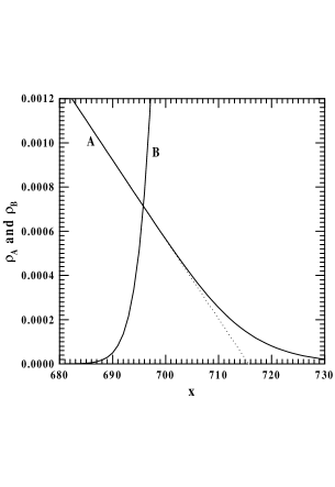
Figure 1: The concentrations $\rho_{\mathrm{A}}$ and $\rho_{\mathrm{B}}$ of A’s and B’s in the vicinity of $x_{\mathrm{f}}\approx 713$ at $t=10^{7}$. The dotted line was computed from (12).

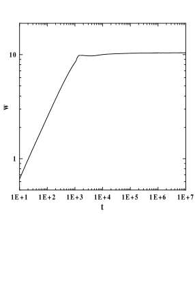
Figure 2: The log-log plot of the width of the reaction front $w$ as a function of time.

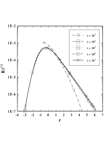
Figure 3: The scaling plot of $R\sqrt{t}$ as a function of $z=(x-x_{\mathrm{f}})/w$.

6 Summary and conclusions

We have investigated the long-time behaviour of the concentrations $\rho_{\mathrm{A}}$ and $\rho_{\mathrm{B}}$ of species A and B in the initially separated diffusion limited systems with $D_{\mathrm{B}}=0$. All of our analysis was carried out for arbitrary values of $D_{\mathrm{A}}$, $a_{0}$ and $b_{0}$.

First we derived the formulae (14) and (15) which together with (12) describe the behaviour of $\rho_{\mathrm{A}}(x,t)$ outside the reaction zone. An interesting feature of these equations is that we expect them to be valid for any reaction-diffusion system of the type A $+$ B(static) $\to$ 0 that exhibits the scaling behaviour with $\alpha<\frac{1}{2}$. Thus we conclude that many important properties of the reaction-diffusion systems with $D_{\mathrm{B}}=0$ depend only on the values of $a_{0}$, $b_{0}$ and $D_{\mathrm{A}}$, but not on the explicit form of $R$. This includes the location of the reaction zone centre (controlled by $C_{\mathrm{f}}$), the total reaction rate (controlled by $C_{\mathrm{J}}$), and the concentration profile of particles A outside the reaction zone (controlled by $C_{\mathrm{A}}$ and $C_{\mathrm{f}}$). A similar situation is observed in the systems with $D_{\mathrm{B}}>0$ [20].

Next we investigated general consequences of the scaling ansatz. We concluded that it determines the value of $\gamma_{\mathrm{B}}=0$ and imposes relations (24) and (26) on the values of $\alpha$, $\beta$ and $\gamma_{\mathrm{A}}$. These relations are also valid for $D_{\mathrm{B}}>0$. We proved that the scaling functions $S_{\mathrm{A}}$ and $S_{\mathrm{B}}$ are related by a simple formula (28). We also concluded that for $D_{\mathrm{B}}=0$ the asymptotic forms of $\rho_{\mathrm{A}}$ and $\rho_{\mathrm{B}}$ inside the reaction front can be derived from equations (19) which are to be solved with time depending boundary conditions (20). Thus these equations determine the asymptotic properties of the reaction front.

We also examined in detail the properties of the reaction zone in the mean-field approximation. In particular we determined the functional forms of $S_{\mathrm{A}}$, $S_{\mathrm{B}}$ and $S_{\mathrm{R}}$ far from $x_{\mathrm{f}}$ and the dependence of the width of the reaction zone on $k$, $a_{0}$, $b_{0}$ and $D_{\mathrm{A}}$.

Our analysis showed that the main differences in the behaviour of the initially separated reaction-diffusion systems with $D_{\mathrm{B}}=0$ and $D_{\mathrm{B}}>0$ arise from the fact that the term $\partial\rho_{\mathrm{B}}/\partial t$ can be neglected in (1) only if the corresponding diffusion constant $D_{\mathrm{B}}$ is nonzero. Therefore, depending on whether $D_{\mathrm{B}}$ is zero or not, the long-time behaviour of the reaction front is governed by entirely different partial differential equations. If $D_{\mathrm{B}}>0$, then we use the usual quasistationary equations (6), otherwise we must employ (19). The different forms of these equations and their boundary conditions imply the different forms of their solutions and, consequently, different asymptotic properties of the two universality classes. Therefore the cases $D_{\mathrm{B}}=0$ and $D_{\mathrm{B}}>0$ should always be considered separately.

There is, however, evidence that in some special cases the two asymptotic universality classes may be very much alike. Such surprising conclusion follows from the extensive numerical simulations of the one dimensional system carried recently out by Cornell [15]. He considered a system with $D_{\mathrm{A}}=D_{\mathrm{B}}>0$ and concluded that $\alpha=1/4$, $\beta=3/4$, and that asymptotically $R$ is a Gaussian centred at $x_{\mathrm{f}}$ with its width growing as $t^{\alpha}$. The same results were derived analytically for the one dimensional system with $D_{\mathrm{B}}=0$ by Larralde et al [14]. Note also that this form of $R$, or more generally — any $R$ that depends on $x$ and $t$ explicitly rather than through $\rho_{\mathrm{A}}(x,t)$ and $\rho_{\mathrm{B}}(x,t)$, uniquely determines the form of $\rho_{\mathrm{A}}(x,t)$. This comes from the fact that whether or not $D_{\mathrm{B}}=0$, asymptotical forms of $\rho_{\mathrm{A}}$ and $R$ are related by the same differential equation $D_{\mathrm{A}}\partial^{2}\rho_{\mathrm{A}}(x,t)/\partial x^{2}=R(x,t)$ with the same boundary conditions. Therefore it is quite possible that the only difference between the one dimensional systems with $D_{\mathrm{B}}=0$ and $D_{\mathrm{B}}>0$ lies in the form of $S_{\mathrm{B}}$ and the value of $\gamma_{\mathrm{B}}$. It should be stressed, however, that the asymptotic kinetics of one dimensional systems with $D_{\mathrm{B}}>0$ has recently become the subject of controversial discussions [15, 16, 17, 25, 26], and further exploration of this topic is still required before the final conclusions can be made.

Acknowledgments
This work was supported by University of Wrocław Grant No 2115/W/IFT/95.

References

- [1] L. Gálfi and Z. Rácz, Phys. Rev. A 38 (1988) 3151.
- [2] Proceedings of the NIH Meeting on Models of Non-Classical Reaction Rates, J. Stat. Phys. 65, No. 5/6, 1991.
- [3] H. Taitelbaum, Y. E. L. Koo, S. Havlin, R. Kopelman and G. H. Weiss, Phys. Rev. A 46 (1992) 2151.
- [4] S. Havlin, M. Araujo, Y. Lereach, H. Larralde, A. Shehter, H. E. Stanley, P. Trunfio and B. Vilensky, Physica A 221 (1995) 1.
- [5] Z. Koza and H. Taitelbaum, Phys. Rev. E 54 (1996) R1040.
- [6] Y. E. Koo and R. Kopelman, J. Stat. Phys. 65 (1991) 893.
- [7] H. Taitelbaum in Diffusion Processes: Experiment, Theory and Simulations, Andrzej Pȩkalski (Ed.), Springer-Verlag, Berlin, 1994.
- [8] S. Cornell and M. Droz, Phys. Rev. Lett. 70 (1993) 3824.
- [9] P. L. Krapivsky, Phys. Rev. E 51 (1995) 4774.
- [10] S. Cornell, M. Droz and B. Chopard, Phys. Rev. A 44 (1991) 4826.
- [11] B. P. Lee and J. Cardy, Phys. Rev. E 50 (1994) R3287.
- [12] M. Howard and J. Cardy, J. Phys. A: Math. Gen. 28 (1995) 3599.
- [13] B. P. Lee and J. Cardy, J. Stat. Phys. 80 (1995) 971.
- [14] H. Larralde, M. Araujo, S. Havlin and H. E. Stanley, Phys. Rev. A 46 (1992) R6121.
- [15] S. J. Cornell, Phys. Rev. E 51 (1995) 4055.
- [16] M. Araujo, H. Larralde, S. Havlin and H. E. Stanley, Phys. Rev. Lett. 71 (1993) 3592.
- [17] G. T. Barkema, M. J. Howard and J. L. Cardy, Phys. Rev. E 53 (1996) R2017.
- [18] M. Hoyuelos, H. O. Mártin and E. V. Albano, J. Phys. A: Math. Gen. 28 (1995) L483.
- [19] E. Ben-Naim and S. Redner, J. Phys. A: Math. Gen. 28 (1992) L575.
- [20] Z. Koza, J. Stat. Phys. 85 (1996) 179.
- [21] Y. L. Luke, Integrals of Bessel Functions, McGraw-Hill, New York, 1962.
- [22] Z. Jiang and C. Ebner, Phys. Rev. A 42 (1990) 7483.
- [23] H. Larralde, M. Araujo, S. Havlin and H. E. Stanley, Phys. Rev. A 46 (1992) 855.
- [24] H. Taitelbaum, S. Havlin, J. E. Kiefer, B. Trus and G. H. Weiss, J. Stat. Phys. 65 (1991) 873.
- [25] S. J. Cornell, Phys. Rev. Lett. 75 (1995) 2250.
- [26] M. Araujo, H. Larralde, S. Havlin and H. E. Stanley, Phys. Rev. Lett. 75 (1995) 2251.