1 Introduction

The admittance determines the current response of an electrical conductor to oscillating voltages applied to its contacts. The admittance and the nonlinear dc-transport have in common that they require both an understanding of the charge distribution which is established as the conductor is driven away from its equilibrium state. The dynamic and the nonlinear transport can thus be viewed as probes of the charge response of the conductor. In contrast, linear dc-transport is determined by the equilibrium charge distribution alone. Thus the dynamic conductance and the nonlinear transport provide information which cannot be gained from a linear dc-measurement.

It is the purpose of this article to provide a discussion of ac-transport and nonlinear transport in small mesoscopic conductors. Our discussion leans heavily on the scattering approach to electrical dc-conductance and can be viewed as an extension of this approach to treat transport beyond the stationary ohmic regime. Our emphasis is on the low-frequency admittance for which expressions can be derived which are very general and can be applied to a large class of problems. Similarly our discussion emphasizes the departure from linear ohmic transport in the case when nonlinearity first becomes apparent. The principles which govern the low-frequency behavior and the weakly nonlinear behavior apply of course as well for high-frequency transport and for strongly nonlinear transport. We underline this fact by treating the simple example of a resonant tunneling barrier for its entire frequency range and by calculating the nonlinear I-V characteristic for a large range of applied voltages.

The general guiding principles of our discussion are charge and current conservation and the need to obtain gauge invariant expressions. The conservation of charge becomes a fundamental requirement under the following condition [1]: Suppose that it is possible to find a volume $\Omega$ which encloses the mesoscopic part of the conductor including a portion of its contacts such that all electric field lines remain within this volume. Clearly, if the mesoscopic conductor is formed with the help of gates the volume $\Omega$ must be large enough to enclose also a portion of the gates. The electric field is then localized within $\Omega$. Such localized electric (and magnetic) field distributions are always implicitly assumed when a circuit is represented simply in terms of $R$, $C$ and $L$ elements. If the field is localized in $\Omega$ the electric flux through the surface of that volume is zero and according to the law of Gauss the total charge inside this volume is zero. Consequently, application of a time-dependent or stationary voltage to the conductor (or a nearby gate) leads only to a redistribution of charge within $\Omega$ but leaves the overall charge invariant. Therefore, a basic ingredient of a reasonable discussion of transport of an electrical conductor is a theory of the charge distribution with the overall constraint that the total charge is conserved. If the total charge is conserved then the currents measured at the contacts of the sample are also conserved. As we will show, this leads to sum rules for the admittance coefficients of a mesoscopic conductor and leads to sum rules for the coefficients which govern the nonlinear dc-transport. The conservation of the total charge is also connected with the fact that an electrical conductor does not change its properties if we shift all potentials by an equal amount. The principle of gauge invariance states that the results can depend only on voltage differences. This leads to a second set of sum rules for the admittance coefficients and for the nonlinear transport coefficients [2].

The three guiding principles which we have taken for the development of a theory are thus very closely related and hinge on the localization of electric and magnetic fields. The existence of a Gauss volume is not, however, a trivial requirement. A different point of view is taken in a recent article by Jackson [3]. In his circuit the potential distribution depends on the location of the battery vis-à-vis the resistor. Such a point of view would make it necessary to develop a theory for the entire circuit including its components used to drive it out of equilibrium. We believe that the notion of localized fields is a more fruitful one and is closer to the experimental reality as it is encountered in mesoscopic physics. In what follows, it is not only assumed that the electric fields are localized, but that the localization volume $\Omega$ is in fact of the same dimension as a phase breaking length. This permits us to formulate a theory for the mesoscopic structure alone and to treat the completion of the circuit as a macroscopic problem.

A charge and current conserving approach to mesoscopic ac-conductance was developed by one of the authors in collaboration with Prêtre and Thomas [4]. Similar work, without an effort to achieve a self-consistent description, was also presented by Pastawski [5] and Fu and Dudley [6]. In Ref. [4] charge and current conservation was achieved by attributing a single self-consistent potential to a conductor. A discussion which treats the potential landscape in a Hartree-like approach was given in Ref. [7] for metallic screening and in Ref. [1] for long range screening appropriate for semiconductors. These two discussions can be extended to include an effective potential as it occurs in density functional theory[8]. Both the limit of a single potential and the case of a continuous potential are important but for many applications the first is to crude and the later is to complex. In this work we will treat an approach which is in between these two: In this generalized discrete potential model the conductor is divided into as many regions as is necessary to capture the main features of the charge and potential distribution. This permits the description of charge distributions which are mainly dipolar or of a more complex higher order multi-polar form. The authors applied such an approach to the low-frequency behavior of quantized Hall samples [9], quantum point contacts [10] and to nonlinear transport [2].

We will only briefly review the scattering approach to electrical conductance, mainly to introduce the notation used in this article. For a more extended discussion of some of the basic elements of the scattering approach we refer the reader to the introductory chapter of this book or to one of the reviews [11, 12, 13, 14]. The advantage of the scattering approach, as formulated by Landauer [15], Imry[11] and one of the authors [16, 17] lies in the conceptually simple prescription of how to model an open system, i.e. how to couple the sample to external contacts which act as reservoirs of charge carriers and provide the source of irreversibility. The self-consistent potential in the context of transport was already of interest to Landauer [18] and is in fact the main issue which distinguishes his early work from preceding works on transmission through tunnel contacts [19]. A more recent discussion of the potential distribution in ballistic mesoscopic conductors is provided by Levinson [20] and technically is closely related to our approach [1]. For the discrete potential model discussed here, the potential distribution can be discussed in a purely algebraic formulation which we will present in some detail. A large portion of this article is devoted to an explicite illustration of our approach. We discuss the low frequency admittance of wires with barriers and the low frequency admittance of quantum point contacts. In particular, we generalize published work on the low frequency admittance of the quantum point contact to investigate the effect of the gates used to form the quantum point contact. The last section of this work presents a discussion of ac-transport and nonlinear transport over a large frequency and voltage regime under the assumption that the only important displacement current is that to a nearby gate.

The discussion of potentials also sheds light on the limits of validity of the scattering approach as it is used to describe dc-transport: The scattering approach is often classified as a noninteracting theory: That is incorrect. Since scattering states can be calculated in an effective potential the range of validity of the scattering approach is at least the same as density functional theory. That makes it possible to include exchange and correlation effects and makes the scattering approach a mean-field theory. As is known, for instance from the BCS-theory of superconductivity, mean-field theories can be very powerful tools which render any remaining deviations very hard to detect.

The low-frequency behavior discussed here should experimentally be accessible with much of the same techniques as those that are used for dc-measurements. We mention here the work of Chen et al. [21] and Sommerfeld et al. [22] on the magnetic field symmetry of capacitances. We mention further a recent experiment by Field et al. [23] who used a quantum dot capacitively coupled to a two-dimensional electron gas to measure the density of states at the metal-insulator transition. In contrast, experiments at high-frequencies require special efforts to couple the signal to the mesoscopic conductor and to measure the response. As examples, we cite here the work by Pieper and Price on the admittance of an Aharonov-Bohm ring [24], investigations of photo-assisted tunneling by Kouwenhoven et al. [25], noise measurements at large frequencies [26], and transport in superlattices [27]. We emphasize that already the low-frequency linear admittance presents a very interesting characterization of the sample. Indeed, we hope, that this article demonstrates that there is considerable room for additional theoretical and experimental work in this area.
Nonlinear dc-effects of interest are asymmetric current-voltage characteristics and rectification [28], the evolution of half-integer conductance plateaus [29, 30], the breakdown of conductance quantization [31], and negative differential conductance and hysteresis [32]. Like in frequency-dependent transport most of the theoretical work shows no concern for self-consistent effects. An exception is a numerical treatment of a tunneling barrier by Kluksdahl et al. [32].
The emphasis on the role of the long-range Coulomb interaction in this work should be contrasted with the recent discussions of mesoscopic transport in the framework of the Luttinger approach. The Luttinger approach treats the short-range interactions only. However, since a one-dimensional wire cannot screen charges completely, a more realistic treatment should include the Coulomb effects. Without the long-range Coulomb interaction the results based on Luttinger models only are not charge and current conserving and are not gauge invariant. In this context we note that the theory of the Coulomb blockade has been very successful in describing the important experimental aspects. The Coulomb blockade is a consequence of long-range and not of short-range interactions. In any case the Hartree discussion given here is useful as a comparison with other theories which include interactions. To distinguish non-Fermi liquid behavior from those of a Fermi liquid it will be essential to compare experimental data with a reasonable, i. e. self-consistent, Fermi liquid theory.

2 Theory

In this section we recall briefly the theory of ac-transport and weakly nonlinear transport which has been developed in Refs. [1, 2, 4, 7, 10]. A review of these works is provided by Ref. [33].

2.1 Mesoscopic Conductors

Consider a conducting region which is connected via leads and contacts $\alpha=1,...,N$ to $N$ reservoirs of charge carriers as shown in Fig. 1a. In order to include into the formalism the presence of nearby gates (capacitors), some parts of the sample are allowed to be macroscopically large and disconnected from other parts. A magnetic field $B$ may be present. It is assumed that the leads of the conducting part are so small that carrier motion occurs via one-dimensional subbands (channels) $m=1,...,M_{\alpha}$ for each contact. Moreover, the distance between these contacts is assumed to be short compared to the inelastic scattering length and the phase-breaking length, such that transmission of charge carriers from one contact to another one can be considered to be elastic and phase coherent. A reservoir is at thermodynamic equilibrium and can thus be characterized by its temperature T_α and by the electrochemical potential $\mu_{\alpha}$ of the carriers. While we assume that all reservoirs are at the same temperature T, we consider differences of the electrochemical potentials which is usually achieved by applying voltages $V_{\alpha}$ to the reservoirs. We fix the voltage scales such that $V_{\alpha}\equiv 0$ corresponds to the equilibrium reference state where all electrochemical potentials of the reservoirs are equal to each other, $\mu_{\alpha}\equiv\mu_{0}$. The problem to be solved is now to find the current $I_{\alpha}(t)$ entering the sample at contact $\alpha$ in response to a (generally time dependent) voltage $V_{\beta}(t)$ at contact $\beta$. The general time-dependent nonlinear transport problem is highly nontrivial and we consider mainly weakly nonlinear dc-transport and linear low-frequency transport.

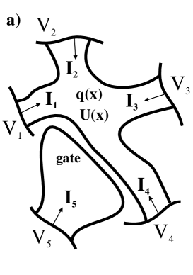
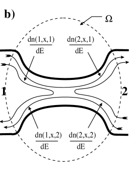
Figure 1.  : a) Multi-terminal sample including a gate; the voltages $V_{\alpha}$ induce charges ($q(x)$) which influence the potential ($U(x)$), and drive currents ($I_{\beta}$). b) Decomposition of the local density of states in a two-terminal sample into local partial densities of states.

2.2 The scattering approach

The sample is described by a unitary scattering-matrix ${\bf S}$ [11, 15, 16, 34]. Unitarity together with micro-reversibility implies that under a reversal of the magnetic field the scattering matrix has the symmetry ${\bf S}^{T}(B)={\bf S}(-B)$ [16, 17]. Furthermore, the scattering matrix ${\bf S}$ for the conductor can be arranged such that it is composed of sub-matrices ${\bf s}_{\alpha\beta}(E,[U(x)])$ with elements $s_{\alpha\beta nm}(E,[U(x)])$ which relate the out-going current amplitude in channel $n$ at contact $\alpha$ to the incident current amplitude in channel $m$ at contact $\beta$. The scattering matrix is a function of the energy $E$ of the carrier and is a functional of the electric potential $U(x)$ in the conductor [1]. For the dc-transport properties, all the physical information which is needed, is contained in the scattering matrix.
The electric potential $U(x,\{V_{\gamma}\})$ is a function of the voltages $V_{\gamma}=(\mu_{\gamma}-\mu_{0})/e$ applied at the contacts and at the nearby gates. Thus the scattering matrix depends not only on the energy of the scattered carriers but also on the voltages, ${\bf s}_{\alpha\beta}(E,\{V_{\gamma}\})$. With the help of the scattering matrix, we can find the current $dI_{\alpha}(E)$ in contact $\alpha$ due to carriers incident at contact $\beta$ in the energy interval $(E,E+dE).$ It is convenient to introduce a spectral conductance [2]

$$g_{\alpha\beta}(E)=\frac{e^{2}}{h}\>Tr[{\bf 1}_{\alpha}(E,\{V_{\gamma}\})\delta_{\alpha\beta}-{\bf s}^{\dagger}_{\alpha\beta}(E,\{V_{\gamma}\}){\bf s}_{\alpha\beta}(E,\{V_{\gamma}\})]$$ (1)

such that the current at energy $E$ becomes $dI_{\alpha}(E)=g_{\alpha\beta}(E)(dE/e).$ The unity matrix ${\bf 1}_{\alpha}$ lives in the space of the quantum channels in lead $\alpha$ with thresholds below the electrochemical potential. Note that this matrix is also a (discontinuous) function of energy and of the potential. It changes its dimension by one whenever the band bottom of a new subband passes the electrochemical potential. The current through contact $\alpha$ is the sum of all spectral currents weighted by the Fermi functions $f(z)=(1+\exp(z/k_{B}{\rm T}))^{-1}$ of the reservoirs [35] at temperature T

$$I_{\alpha}=\sum_{\beta=1}^{N}\int(dE/e)\>f(E-\mu_{0}-eV_{\beta})\>g_{\alpha\beta}(E,\{V_{\gamma}\})\;\;.$$ (2)

Linear transport is determined by an expansion of Eq. (2) away from the equilibrium reference state to linear order in $V_{\gamma}$. The linear conductance is found to be

$$G_{\alpha\beta}^{(0)}=\int dE\>(-\partial_{E}f_{0})\;g_{\alpha\beta}(E)\;\;,$$ (3)

where the $G_{\alpha\beta}$ are evaluated at $V_{1}=...=V_{N}=0$. Consequently, the linear conductances depend on the equilibrium electrostatic potential $U^{(eq)}(x)\equiv U(x,\{0\})$ only. In contrast, both the ac-transport and the nonlinear transport depend explicitly on the nonequilibrium potential. A discussion of the nonequilibrium potential requires knowledge of the local charge distribution in the conductor. Within linear response, the charge response is related to the DOS of the conductor at the Fermi energy. The local DOS can be obtained from the scattering matrix by a functional derivative with respect to the local potential [1]

$$\frac{dn(x)}{dE}=-\frac{1}{4\pi i}\sum_{\alpha\beta}Tr\left[{\bf s}^{\dagger}_{\alpha\beta}\frac{\delta{\bf s}_{\alpha\beta}}{e\delta U(x)}-\frac{\delta{\bf s}^{\dagger}_{\alpha\beta}}{e\delta U(x)}{\bf s}_{\alpha\beta}\right]\equiv\sum_{\alpha\beta}\frac{dn(\alpha,x,\beta)}{dE}\;\;.$$ (4)

As indicated in Eq. (4), the local DOS can be understood as a sum of local partial densities of states (PDOS) $dn(\alpha,x,\beta)/dE$ [36]. The sum is over all injecting contacts $\beta$ and all emitting contacts $\alpha$. The meaning of a local PDOS $dn(\alpha,x,\beta)/dE$ is then obvious: it is the local density of states associated with carriers which are scattered from contact $\beta$ to contact $\alpha$. The local PDOS are illustrated in Fig. 1b. The global DOS, $dN/dE$, follows by a spatial integration of Eq. (4) over the sample region $\Omega$ which encloses the mesoscopic structure with a boundary deep inside the reservoirs. Integration of the local PDOS over the whole sample leads to the global PDOS, $dN_{\alpha\beta}/dE$. Clearly, it holds $dN/dE=\sum_{\alpha\beta}dN_{\alpha\beta}/dE$. Note that Eq. (4) counts only scattering states. Pure bound states, e.g. trapped or pinned at an impurity, are not included.
The local PDOS $dn(x,\beta)/dE$ which contains information only on the contact from which the carriers enter the conductor (irrespectively of the contact through which the carriers exit) is called the injectivity of contact $\beta$ and is given by $dn(x,\beta)/dE=\sum_{\alpha}dn(\alpha,x,\beta)/dE$. The local PDOS $dn(\alpha,x)/dE$ which contains information only on the contact through which carriers are leaving the sample but contains no information on the contact through which carriers entered the conductor is called the emissivity of contact $\alpha$ and is given by $dn(\alpha,x)/dE=\sum_{\beta}dn(\alpha,x,\beta)/dE$. Due to reciprocity, the injectivity at a magnetic field $B$ is equal to the emissivity at the reversed magnetic field, $dn_{B}(x,\alpha)/dE=dn_{-B}(\alpha,x)/dE$.
Throughout this work we use the discrete potential approximation in which the conductor is divided into $M$ regions $\Omega_{k}$, $k=1,...,M$. The charge and the potential in region $k$ are denoted by $q_{k}$ and $U_{k}$. Since we are are interested in the charge variation in response to a variation in voltage, we introduce the DOS of $\Omega_{k}$. For later convenience, we express these DOS in units of a capacitance by multiplication with $e^{2}$. Thus, $D_{k}=e^{2}\int_{\Omega_{k}}dx\>(dn(x)/dE)$ is the DOS of region $k$. The PDOS of region $k$ are $D_{\alpha k\beta}=e^{2}\int_{\Omega_{k}}dx\>(dn(\alpha,x,\beta)/dE)$. Obviously, the injectivities and the emissivities are $D_{k\beta}=e^{2}\int_{\Omega_{k}}dx\>(dn(x,\beta)/dE)$ and $D_{\alpha k}=e^{2}\int_{\Omega_{k}}dx\>(dn(\alpha,x)/dE)$, respectively.

2.3 Linear low-frequency transport

We are interested in the admittance $G_{\alpha\beta}(\omega)$ which determines the Fourier amplitudes of the current, $\delta I_{\alpha}(\omega)$, at a contact $\alpha$ in response to an oscillating voltage $\delta V_{\beta}(\omega)\exp(-i\omega t)$ at contact $\beta$

$$\delta I_{\alpha}=\sum_{\beta}G_{\alpha\beta}(\omega)\;\delta V_{\beta}\;\;.$$ (5)

To investigate the low-frequency limit, we expand the admittance in powers of frequency

$$G_{\alpha\beta}(\omega)=G_{\alpha\beta}^{(0)}-i\omega E_{\alpha\beta}+\omega^{2}K_{\alpha\beta}+{\cal O}(\omega^{3})\;\;.$$ (6)

The dc-conductance $G_{\alpha\beta}^{(0)}$ has already been derived in Eq. (3). The first order term is determined by the emittance matrix $E_{\alpha\beta}\equiv i(dG_{\alpha\beta}/d\omega)_{\omega=0}$. The emittance governs the displacement currents of the mesoscopic structure. The second order term, $K_{\alpha\beta}$, contains information on the charge relaxation of the system. As an example, consider for a moment a macroscopic capacitor $C$ in series with a resistor $R$. For this purely capacitive structure with vanishing dc-conductance, $G=0$, the emittance is the capacitance, $E=C$, and $K=R^{(q)}C^{2}$ contains the $RC$ time with the charge relaxation resistance $R^{(q)}\equiv R$. More generally, for any structure consisting of $N$ metallic conductors, each connected to a single reservoir, the emittance matrix is just the capacitance matrix. These simple results must be modified for mesoscopic conductors and conductors which connect different reservoirs. Firstly, it is not the geometrical capacitance but rather the DOS dependent electro-chemical capacitance which relates charges on mesoscopic conductors to voltage variations in the reservoirs [37]. Secondly, conductors which connect different reservoirs allow a transmission of charge which leads to inductance-like contributions to the emittance [1, 4, 10]. Thirdly, the charge relaxation resistance cannot, in general, be calculated like a dc-resistance [37, 38].
To illustrate our approach, we derive now a general expression for the emittance. We first notice that for the purely capacitive case the current (displacement current) at contact $\alpha$ is the time derivative of the total charge $\delta Q_{\alpha}$ on the capacitor plates connected to this contact. Hence, $\delta I_{\alpha}=-i\omega\delta Q_{\alpha}$ and the emittance is given by $E_{\alpha\beta}=\partial Q_{\alpha}/\partial V_{\beta}$. If transmission between different reservoirs is allowed, the charge $\delta Q_{\alpha}$ scattered through a contact can no longer be associated with a unique spatial region. The charge at a given point is rather injected at different contacts and ejected at different contacts. However, the charge emitted at a contact can still be calculated within the scattering approach. We decompose it in a bare and a screening part $\delta Q_{\alpha}=\delta Q_{\alpha}^{(b)}+\delta Q_{\alpha}^{(s)}$. The bare part of the charge corresponds to the charge which is scattered through the contact $\alpha$ for fixed electric potential and is thus given by

$$\delta Q_{\alpha}^{(b)}=\sum_{\beta}D_{\alpha\beta}\delta V_{\beta}\;\;,$$ (7)

where $D_{\alpha\beta}=\sum_{k}D_{\alpha k\beta}$ is the global PDOS. The screening part, on the other hand, is associated with the charge which is scattered through contact $\alpha$ for a variation in the electric potential only. Since a shift of the band bottom contributes with a negative sign and since the potential is in general spatially varying, $\delta Q_{\alpha}^{(s)}$ is connected to the local PDOS by $\delta Q_{\alpha}^{(s)}=-\sum_{k}D_{\alpha k}\delta{U}_{k},$ where $D_{\alpha k}$ is the emissivity of region $k$ into contact $\alpha$. If we introduce the vector of emissivities ${\bf D}^{e}_{\alpha}=(D_{\alpha 1},..,D_{\alpha M})$ and write the potential variation as a vector, $\delta{\bf U}=(\delta{U}_{1},....,\delta{U}_{M})$, the charge emitted into contact $\alpha$ is

$$\delta Q_{\alpha}^{(s)}=-{\bf D}^{e}_{\alpha}\delta{\bf U}\;\;.$$ (8)

In linear response the potential variation $\delta{\bf U}$ is linearly related to the potential variations $\delta V_{\beta}$ at the contacts of the sample. We write

$$\delta{\bf U}=\sum_{\alpha}{\bf u}_{\alpha}\>\delta V_{\alpha}\;\;$$ (9)

where the response coefficients ${\bf u}_{\alpha}=(u_{1\alpha},...,u_{M\alpha})$ are called the characteristic potentials of contact $\alpha$. The emittance can be written as

$$E_{\alpha\beta}=D_{\alpha\beta}-{\bf D}^{e}_{\alpha}{\bf u}_{\beta}\;\;.$$ (10)

To complete the calculation of the emittance, we next need a discussion of the characteristic potentials.

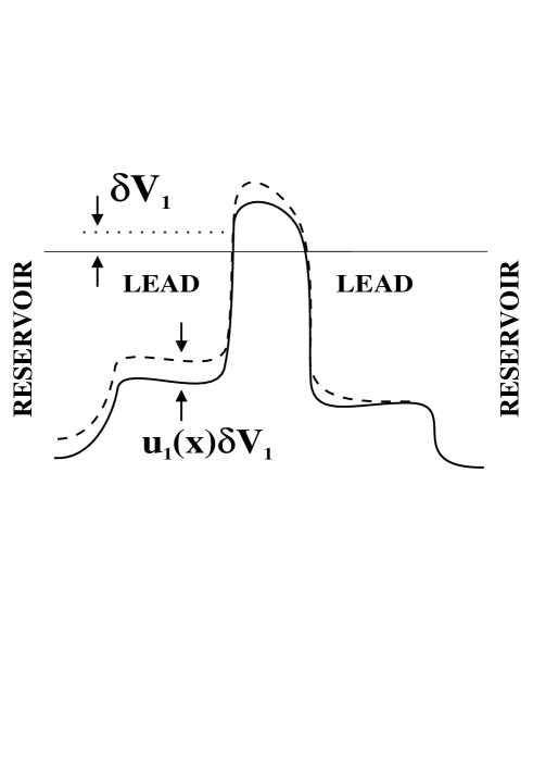
Figure 2.  : Change (dashed) of the equilibrium potential (solid) in a two-terminal sample due to a voltage variation $\delta V_{1}$ (dotted) in the left reservoir.

2.4 Piled-up charge and self-consistent potential

The variation of the charge $\delta q_{k}$ is the sum of a bare charge and a screening charge. The bare charge can be expressed with the help of the injectivity

$$\delta{\bf q}^{(b)}=\sum_{\beta}{\bf D}^{i}_{\beta}\;\delta V_{\beta}\;\;.$$ (11)

The screening charge is connected to the electrostatic potential [20] via the Lindhard polarization function, which is here a matrix ${\bf\Pi}$ with elements $\Pi_{kl}$,

$$\delta{\bf q}^{(s)}=-{\bf\Pi}\>{\bf\delta U}\;\;.$$ (12)

The Lindhard matrix can be expressed in terms of the scattering states. It is in general not a diagonal matrix, i.e. the charge response is in general nonlocal. Non-local effects are, however, small quantum mechanical effects which can be neglected deep inside a conductor with a sufficiently large electron density. In a quasiclassical treatment the Lindhard matrix becomes local, $\Pi_{kl}=\delta_{kl}D_{k}$. Here $D_{k}$ is the local DOS in region $k$.
The total charge, $\delta{\bf q}=\delta{\bf q}^{(b)}+\delta{\bf q}^{(s)}$, acts now as the source of the nonequilibrium electric potential in the Poisson equation. For our discrete model we also have to discretize the Poisson equation. We introduce a geometrical capacitance matrix ${\bf C}$ which relates the charges to the electrostatic potentials, $\delta{\bf q}={\bf C}\delta{\bf U}$. If one uses this matrix ${\bf C}$ and expresses the electric potential in terms of the characteristic potentials, one can write the Poisson equation in the form $({\bf C}+{\bf\Pi}){\bf u}_{\alpha}={\bf D}^{(i)}_{\alpha}$ which determines the characteristic potentials ${\bf u}_{\alpha}$,

$${\bf u}_{\alpha}=({\bf\Pi}+{\bf C})^{-1}{\bf D}^{(i)}_{\alpha}\;\;.$$ (13)

Going back to Eq. (10) we find for the emittance

$$E_{\alpha\beta}=D_{\alpha\beta}-{\bf D}^{(e)}_{\alpha}({\bf\Pi}+{\bf C})^{-1}{\bf D}^{(i)}_{\beta}\;\;.$$ (14)

We notice that the bare contribution to the emittance occurs with a positive sign and the Coulomb induced contribution occurs with a negative sign. Depending on which contribution dominates we call the emittance element capacitive ($E_{\alpha\alpha}>0$, $E_{\alpha\beta}<0$ for $\alpha\neq\beta$) or inductive-like ($E_{\alpha\alpha}<0$, $E_{\alpha\beta}>0$ for $\alpha\neq\beta$).
The nonequilibrium charge distribution becomes

$$\delta{\bf q}={\bf C}\delta{\bf U}=\sum_{\beta}{\bf D}^{(i)}_{\beta}\delta V_{\beta}-{\bf\Pi}\delta{\bf U}\;\;.$$ (15)

This determines the nonequilibrium steady-state to linear order in the applied voltages. The nonequilibrium charge-distribution can be written in terms of an electrochemical capacitance matrix $C_{\mu,k\beta}$ [2, 9, 10] which determines the net charge variation in region $k$ in response to a potential variation at contact $\beta$. In vector notation, we have

$$\delta{\bf q}=\sum_{\beta}{\bf C}_{\mu,\beta}\delta V_{\beta}\;\;,$$ (16)

where

$${\bf C}_{\mu,\beta}={\bf C}{\bf u}_{\beta}={\bf C}({\bf\Pi}+{\bf C})^{-1}{\bf D}^{(i)}_{\beta}\;\;.$$ (17)

We do not present here a general discussion of the charge relaxtion term $K_{\alpha\beta}$. This requires a dynamical screening theory, and we have results only for special cases. We discuss one of these special cases in Sect. 2.7 and Sect. 3.3.

2.5 Weakly nonlinear dc-transport

The nonequilibrium potential distribution is not only of importance in ac-transport but also in nonlinear transport. Knowledge of the nonequilibrium potential distribution to first order in the applied voltages permits to find the nonlinear I-V-characteristic up to quadratic order in the voltages,

$$I_{\alpha}=\sum_{\beta}G_{\alpha\beta}^{(0)}V_{\beta}+\sum_{\beta\gamma}G_{\alpha\beta\gamma}^{(0)}V_{\beta}V_{\gamma}+{\cal O}(V^{3})\;\;.$$ (18)

The coefficients $G_{\alpha\beta}^{(0)}$ and $G_{\alpha\beta\gamma}^{(0)}$ are obtained from an expansion of Eq. (2) with respect to the voltages $V_{\alpha}$. One obtains for the linear conductance Eq. (3). An expansion of Eq. (2) up to ${\cal O}(V^{2})$ yields $G_{\alpha\beta\gamma}^{(0)}=(1/2)\int dE\>(-\partial_{E}f)$ $\left(2\partial_{V_{\gamma}}g_{\alpha\beta}+e\partial_{E}g_{\alpha\beta}\delta_{\beta\gamma}\right)$. Writing $\partial_{V_{\gamma}}g_{\alpha\beta}$ in terms of the derivatives $dg_{\alpha\beta}/dU_{k}$ and the characteristic potentials yields

$$G_{\alpha\beta\gamma}^{(0)}=\frac{1}{2}\int dE\>(-\partial_{E}f)\sum_{k}\>\frac{dg_{\alpha\beta}}{dU(k)}\left(2u_{k\gamma}-\delta_{\beta\gamma}\right)\;\;.$$ (19)

Expressing the characteristic potentials in terms of the injectivities we find that the rectification coefficient is given by

$$G_{\alpha\beta\gamma}^{(0)}=\frac{1}{2}\int dE(-\partial_{E}f)\left(2({\bf\nabla_{U}}g_{\alpha\beta})^{t}\>({\bf\Pi}+{\bf C})^{-1}{\bf D}^{(i)}_{\gamma}+e\delta_{\beta\gamma}\partial_{E}g_{\alpha\beta}\right)\;\;.$$ (20)

For a quantum point contact, Eq. (20) has been discussed in Ref. [2]. In Sect. 3.3 we will apply this result to the resonant tunneling barrier.

2.6 Charge conservation, gauge invariance, and Magnetic Field Symmetry

Since the system under consideration includes all conductors and nearby gates, the theory must satisfy charge (and current) conservation and gauge invariance. Due to micro-reversibility the linear response matrices must additionally satisfy the Onsager-Casimir symmetry relations.
Let us first discuss charge conservation, which states that the total charge in the sample remains constant under a bias. This implies also current conservation, $\sum_{\alpha}I_{\alpha}=0$. Imagine a volume $\Omega$ which encloses the entire conductor including a portion of the reservoirs which is so large that at the place were the surface of $\Omega$ intersects the reservoir all the characteristic potentials are either zero or unity. According to the law of Gauss, one concludes that the total charge remains constant. Application of a bias voltage results only in a redistribution of the charge. If the conductor is poor, i.e. nearly an insulator, the contacts act like plates of capacitors. In this case long-range fields exist which run from one reservoir to the other and from a reservoir to a portion of the conductor. But if we chose the volume $\Omega$ to be large enough then all field lines stay within this volume. Charge and current conservation imply for the response coefficients the sum rules

$$\sum_{k}C_{\mu,k\beta}=\sum_{\alpha}G_{\alpha\beta}^{(0)}=\sum_{\alpha}E_{\alpha\beta}=\sum_{\alpha}K_{\alpha\beta}=\sum_{\alpha}G_{\alpha\beta\gamma}^{(0)}=0\;\;.$$ (21)

Second consider the fact that only voltage differences are physically meaningful. Gauge invariance means that measurable quantities are invariant under a global voltage shift $\delta V$ in the reservoirs, $\delta V_{\alpha}\mapsto\delta V_{\alpha}+\delta V$. A global voltage shift corresponds, of course, only to a change of the global voltage scale. Consequently, the characteristic potentials satisfy [37]

$$\sum_{\alpha}{\bf u}_{\alpha}={\bf 1}\;\;.$$ (22)

For the response coefficients the following sum rules hold

$$\sum_{\beta}C_{\mu,k\beta}=\sum_{\beta}G_{\alpha\beta}^{(0)}=\sum_{\beta}E_{\alpha\beta}=\sum_{\beta}K_{\alpha\beta}=\sum_{\beta}(G_{\alpha\beta\gamma}^{(0)}+G_{\alpha\gamma\beta}^{(0)})=0\;\;.$$ (23)

Note that due to charge conservation and gauge invariance, the geometrical capacitance matrix ${\bf C}$ has the zero mode ${\bf 1}=(1,1,....1)$, corresponding to a unit potential in each region. Thus ${\bf C}$ cannot be inverted. However, the Green’s function $({\bf\Pi}+{\bf C})^{-1}$ which solves the Poisson equation exists (see Eq. (13)). Expressing the characteristic potentials with the help of the Green’s function and the injectivities gives

$${\bf 1}=({\bf\Pi}+{\bf C})^{-1}{\bf D}\;\;$$ (24)

where ${\bf D}=(D_{1},D_{2},...,D_{M})$ is the vector of the local DOS. Equation (24) is the key property of the Green’s function needed to show that our final results are charge and current conserving. From Eq. (24) it follows immediately that the sum over the elements of a row of the Lindhard matrix is equal to the DOS in region $k$, i.e. $D_{k}=\sum_{l}\Pi_{kl}$. Since the Lindhard matrix is symmetric, it holds also $D_{k}=\sum_{l}\Pi_{lk}$. The above mentioned statement, that in the quasiclassical local case $\Pi_{kl}=D_{k}\delta_{kl}$ holds, is now clear.
In the presence of a magnetic field, the admittance matrix must additionally satisfy the reciprocity relations

$$G_{\alpha\beta}(\omega)|_{B}=G_{\beta\alpha}(\omega)|_{-B}\;\;$$ (25)

which is a consequence of time-reversal symmetry of the microscopic equations and the fact that we consider transmission from one reservoir to another [1, 16, 17]. These Onsager-Casimir relations are only valid for the linear response coefficients, i.e. close to equilibrium. Of course, the symmetry relations (25) hold individually for $G_{\alpha\beta}^{(0)}$, $E_{\alpha\beta}$, and $K_{\alpha\beta}$. Note that the emittance is symmetric, $E_{\alpha\beta}=E_{\beta\alpha}$, in the purely capacitive case.

2.7 Frequency-Dependent Transport: Single Potential Approximation

In this section we show that it is possible to discuss the full frequency-dependence of the admittance, if the electric potential in the mesoscopic conductor can be approximated by a single variable. The external response is defined as the response for fixed electrostatic potential (i.e. the ‘bare’ response). A general result for the external response has been derived in Ref. [4]. If the differences of wave vectors $k(E)$ and $k(E+\hbar\omega)$ deep in the reservoirs are neglected, the external response can be expressed in terms of the scattering matrix only,

$$G_{\alpha\beta}^{e}(\omega)=\frac{e}{h}\int dETr[{\bf 1}_{\alpha}\delta_{\alpha\beta}-{\bf s}^{\dagger}_{\alpha\beta}(E){\bf s}_{\alpha\beta}(E+\hbar\omega)]\frac{(f(E)-f(E+\hbar\omega))}{\hbar\omega}\;\;.$$ (26)

The scattering matrices and the Fermi functions are here evaluated at the equilibrium reference state. The real part of the ac-conductance, (26) is related via the fluctuation-dissipation theorem to the current-current fluctuation spectra derived in Ref. [39]. An expansion of Eq. (26) to linear order in $\omega$ gives [4]

$$G_{\alpha\beta}^{e}(\omega)=G_{\alpha\beta}^{(0)}-i\omega{e^{2}}\int dE\>(-df/dE)\>(dN_{\alpha\beta}/dE)\;\;,$$ (27)

where the $dN_{\alpha\beta}/{dE}$ are the global PDOS, in which the functional derivative with respect to the local potential (and the integration over the volume $\Omega$) is replaced by a (negative) energy derivative. Asymptotically, for a large volume $\Omega$ the global PDOS obtained from an energy derivative is identical to the integral of the local PDOS associated with a functional derivative with respect to the potential according to Eq. (4). However, for a finite volume, there are typically small differences of the order of the Fermi wavelength divided by the size of the volume $\Omega$. For a more detailed discussion, we refer the reader to Ref. [36].
In order to obtain the full admittance, we have still to find the internal response (the ‘screening’ part of the admittance). A general result for the internal response is not known. In the simple case, where the conductor is treated with a single discrete region ($M=1$), the external response defines, however, also the internal response. We assume that the sample is in close proximity to a gate which couples capacitively to the conductor with a capacitance coefficient $C$. The current response at contact $\alpha$ is $\delta I_{\alpha}(\omega)=\sum G^{e}_{\alpha\beta}(\omega)\delta V_{\beta}+G^{i}_{\alpha}(\omega)\delta U_{1}$ where $G^{i}_{\alpha}(\omega)$ is the (unknown) internal response of the conductor generated by the oscillating electrostatic potential $\delta U_{1}$. The current induced into the gate is $\delta I_{g}(\omega)=-i\omega C(\delta V_{g}-\delta U_{1})$. Now we can determine $G^{i}_{\alpha}(\omega)$ from the requirement of gauge invariance. In particular, if all potentials are shifted by $-\delta U_{1}$, it follows immediately that $G^{i}_{\alpha}(\omega)=-\sum_{\beta}G^{e}_{\alpha\beta}(\omega)$. Using current conservation, $\sum_{\alpha}\delta I_{\alpha}+\delta I_{g}=0$, we find for the conductances [4] of the interacting system ($\alpha,\beta,\gamma,\delta\neq g$),

$$G^{I}_{\alpha\beta}(\omega) = G^{e}_{\alpha\beta}(\omega)-\frac{(i/\omega C)\sum_{\gamma}G^{e}_{\alpha\gamma}(\omega)\sum_{\delta}G^{e}_{\delta\beta}(\omega)}{1+(i/\omega C)\sum_{\gamma\delta}G^{e}_{\gamma\delta}(\omega)},$$ (28)

$$G^{I}_{g\beta}(\omega) = -\frac{\sum_{\delta}G^{e}_{\delta\beta}(\omega)}{1+(i/\omega C)\sum_{\gamma\delta}G^{e}_{\gamma\delta}(\omega)},$$ (29)

$$G^{I}_{\alpha g}(\omega) = -\frac{\sum_{\gamma}G^{e}_{\alpha\gamma}(\omega)}{1+(i/\omega C)\sum_{\gamma\delta}G^{e}_{\gamma\delta}(\omega)},$$ (30)

$$G^{I}_{gg}(\omega) = -\frac{\sum_{\gamma\delta}G^{e}_{\gamma\delta}(\omega)}{1+(i/\omega C)\sum_{\gamma\delta}G^{e}_{\gamma\delta}(\omega)}.$$ (31)

The single-potential approximation provides a reasonable description only if the conductor has a well-defined interior region, which might be described by a single uniform potential. Furthermore, it is assumed that the only relevant capacitance is that of the sample and the gate. Examples for which this approach is reasonable are quantum wells or quantum dots or cavities for which the Coulomb interaction is so weak that single electron effects can be neglected. In Section 3.3 we discuss the case of a double barrier with a well which is capacitively coupled to a gate.

3 Examples

In a first example we discuss the emittance of a wire which contains a single barrier. The wire is capacitively coupled to a gate. As a second example we discuss the capacitance and emittance of a quantum point contact formed with the help of gates [10]. It turns out that steps in the capacitance and the emittance occur in synchronism with the well-known conductance steps. As a third example, we treat the resonant tunneling barrier close to a resonance, for which we calculate the nonlinear current-voltage characteristic and the frequency-dependent conductance [2] with the single-potential approximation. For all examples, we use explicit expressions for the Lindard function (matrix) ${\bf\Pi}$ given within the local Thomas-Fermi approximation, where ${\bf\Pi}$ is diagonal with elements determined by the local DOS. In all examples we consider finally the zero-temperature limit.

3.1 Admittance of a wire with a Barrier

Our first example is a mesoscopic wire which connects two contacts and is capacitively coupled to a nearby gate (see Fig. 3). The wire is assumed to be perfect with a uniform potential along its main direction, except for a single scatterer, a barrier, or an impurity. The discussion is carried out in the semiclassical limit where Friedel oscillations are neglected. We take the potential of the impurity to be of short-range and assume that the potential to left and right of the scatter can be assumed to be uniform. We assume here that the gate couples to the wire only and neglect scattering at the interface of the wire and the reservoir. Furthermore, to simplify the discussion we assume in this section that the capacitance between the charges to the left and the right of the barrier can be neglected (i.e. vanishingly small $C_{12}$). Consider first a perfect wire ($T=1$) of length $L$. The gate couples with a geometrical capacitance $c$ per length.

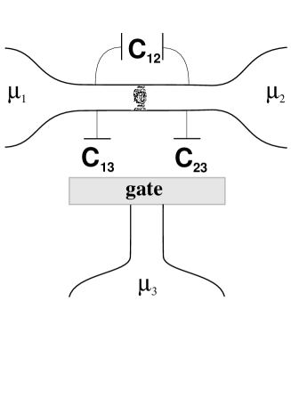
Figure 3.  : Quantum wire containing an impurity and coupled to a gate.

The DOS per length for a one-dimensional wire is

$$dn/dE=2/hv$$ (32)

where $v=(2/m)^{1/2}(E-eU)^{1/2}$ is the velocity of carriers with energy $E$. If the wire is filled up to the electrochemical potential $\mu$ of the reservoirs the total number $n$ of states per length is

$$n(\mu)=\int_{eU}^{\mu}dE(dn/dE)=e^{-1}(2/\pi^{2}a_{B})^{1/2}(\mu-eU)^{1/2}.$$ (33)

Here we have introduced the Bohr radius $a_{B}=\hbar^{2}/me^{2}$. To determine this density self-consistently we consider the Poisson equation. The difference of the electron charge density $en$ and the ionic background charge density $-en^{+}$ is equal to the capacitive charge,

$$en(\mu)-en^{+}=c(U-U_{g})\;\;,$$ (34)

where $U_{g}$ is the electrostatic potential of the gate. Similarly, near its surface, the deviation of the electronic gate charge away from charge neutrality is equal to $-c(U-U_{g})$. Now we take the gate to be a macroscopic conductor. Therefore, the electrostatic potential and the electrochemical potential are everywhere related by $\mu_{g}=E_{Fg}+eU_{g}$, where $E_{Fg}$ is the chemical potential (Fermi energy) of the gate. We eliminate the gate potential $U_{g}$ in Eq. (34) and find

$$en(\mu)=(c/e)(e^{2}n^{+}/c+E_{Fg}-\mu_{g}+eU)\;\;.$$ (35)

Measuring energies from the band bottom of the one-dimensional wire and setting $eU=0$ gives the electrochemical potential as a function of the gate potential,

$$\mu=(c/e)^{2}(\pi^{2}a_{B}/2)(e^{2}n^{+}/c+E_{Fg}-\mu_{g})^{2}\;\;.$$ (36)

In the limit $c\to 0$ the electrochemical potential of the wire is simply determined by charge neutrality, $\mu=$ $(\pi^{2}a_{B}/2)e^{2}$ $(n^{+})^{2}$. For $\mu_{g}=\mu_{0}\equiv e^{2}n^{+}/c+E_{Fg}$ the electrochemical potential vanishes and the wire is empty for $\mu_{g}\geq\mu_{0}$. The DOS of left moving carriers, $dn_{l}/dE=1/hv$, is directly related to the phase accumulated by the electrons traversing the wire, $Ldn_{l}/dE=L/hv=(1/\pi)d\phi/dE$. The phase accumulated by a traversing electron (at the Fermi energy) is thus given by

$$\phi=\pi L(c/e^{2})(e^{2}n^{+}/c+E_{Fg}-\mu_{g})\;\;.$$ (37)

The scattering matrix element for the transmitting channel is given by $s_{21}=\exp(i\phi)$ which shows that the scattering matrix and thermodynamics are intimately related. At the Fermi energy of the wire, the DOS is given by

$$dn/dE=(1/2\pi^{2}a_{B})(1/c)(e^{2}n^{+}/c+E_{Fg}-\mu_{g})^{-1}.$$ (38)

The true electron density in a narrow energy interval at the Fermi energy is found by considering a small variation of the electrochemical potentials $\delta\mu$ and $\delta\mu_{g}$ and the electric potential $\delta U$ away from a reference state ($\mu^{(eq)}$, $\mu_{g}^{(eq)}$, $U^{(eq)}$) which obeys Eq. (35). Variation of this equation gives

$$\delta q=e(dn/dE)(\delta\mu-e\delta U)=c(\delta U-\delta\mu_{g}/e).$$ (39)

Solving for $\delta U$ gives for the charge $\delta q=c_{g}(\delta\mu/e-\delta\mu_{g}/e)$ with an electrochemical wire-to-gate capacitance

$$c^{-1}_{g}=c^{-1}+(e^{2}(dn/dE))^{-1}\;\;.$$ (40)

Here the DOS appears in series with the geometrical capacitance It depends on the reference state and is given by Eq. (38) with $\mu_{g}=\mu^{eq}_{g}.$
Next, we discuss a wire containing a symmetric barrier. At equilibrium, and if we can treat the potential created by the barrier as short-range, the DOS to the left and right of the barrier remains unchanged. Hence the consideration given above for the electrostatic equilibrium potential also characterizes the wire to the left and right of the barrier. Similarly, for a long wire the gate-to-wire capacitance is essentially unaffected by the presence of the barrier. In the case of transport, on the other hand, the chemical potentials of the reservoirs connected to the wire differ by a small amount implying a variation of the charge distribution. We introduce two regions $\Omega_{1}$ and $\Omega_{2}$ of size $L/2$ to the left and the right of the barrier, respectively. With the help of Fig. 1b, the semiclassical local PDOS, $D_{\alpha k\beta}$, can be constructed with simple arguments. For example, $D_{211}$ is given by the transmission probability times the DOS of $\Omega_{1}$ associated with carriers with positive velocity, hence $D_{211}=TD_{1}/2$, with $D_{1}=D_{2}=D/2$ due to symmetry. To determine $D_{212}$, we note that in the semiclassical limit considered here, there are no states in $\Omega_{1}$ associated with scattering from contact $2$ back to contact $2$, hence it holds $D_{212}=0$. With similar arguments one finds for the semi-classical PDOS

$$D_{\alpha k\beta}=D_{k}\left(T/2+\delta_{\alpha\beta}(R\>\delta_{\alpha k}-T/2)\>\right)\;\;,\;\;\;{\rm if}\;\;\alpha,\beta\neq 3\;\;.$$ (41)

Form Eq. (41) we obtain for the emissivities and injectivities $D^{e}_{11}=D^{i}_{11}=(1/4)(1+R)D$ and $D^{e}_{12}=D^{i}_{12}=(1/4)TD$. The integrated geometrical capacitance is denoted by $C=cL$. With these quantities the Poisson equation reads

$$(D/2)(1+R)\delta V_{1}+(TD/2)\delta V_{2}-D\delta U_{1} = C(\delta U_{1}-\delta U_{3})$$

$$(TD/2)\delta V_{1}+(1+R)(D/2)\delta V_{2}-D\delta U_{2} = C(\delta U_{2}-\delta U_{3})$$ (42)

These equations can also be derived by noticing that the variations $\delta F_{k}$ of the quasi-Fermi levels [34] in the regions $k=1$ and $2$ are given by $\delta F_{1}=((1+R)\delta V_{1}+T\delta V_{2})/2$ and $\delta F_{2}=((1+R)\delta V_{2}+T\delta V_{1})/2$, respectively. For a local Lindhard function, the charge in region $k$ is then $\delta q_{k}=D_{k}(\delta F_{k}-\delta U_{k})=(C/2)(\delta U_{k}-\delta U_{3})$.
For the charge neutral case, $C=0$, Eqs. (42) are familiar from Landauer’s discussion of the potential drop across a barrier [15, 18, 34]. We assume again that the gate is a massive conductor for which we have $\mu_{3}=E_{Fg}+eU_{3}$ everywhere. We use Eqs. (42) to evaluate the characteristic potentials and get

$$u_{11}=\frac{1}{2}\frac{(1+R)D}{C+D}, u_{12}=\displaystyle\frac{1}{2}\frac{TD}{C+D}, u_{13}=\frac{C}{C+D}\;\;.$$ (43)

Due to symmetry, it holds $u_{22}=u_{11}$, $u_{21}=u_{12}$ and $u_{23}=u_{13}$. Defining $\Delta V\equiv\delta V_{1}-\delta V_{2}$, the potential drop across the barrier can be written in the form

$$\Delta U\equiv\delta U_{1}-\delta U_{2}=(C_{g}/C)R\Delta V$$ (44)

where $C_{g}=Lc_{g}$ is the electro-chemical gate-to-wire capacitance given by Eq. (40). The voltage difference $\Delta U$ is proportional to the reflection probability $R$ and the chemical potential difference of the reservoirs. The total charges to the left or to the right of the barrier are the sum of the injected charges and the induced charges

$$\delta q_{k}=\sum_{\beta}(D^{i}_{k\beta}-D_{k}u_{k\beta})\delta V_{\beta}\;\;.$$ (45)

We find, e.g., for $\delta q_{1}$,

$$\delta q_{1}=C_{g}\{(1/2)(1+R)\delta V_{1}+(T/2)\delta V_{2}-\delta V_{3}\}.$$ (46)

The difference in the charge density on the left and the right hand side becomes

$$\Delta q\equiv\delta q_{1}-\delta q_{2}=C_{g}R\Delta V.$$ (47)

In the limit of vanishing gate-to-wire capacitance, the charge difference vanishes also. Away from the barrier the wire is charge neutral. In this charge-neutral limit the potential difference is determined by the reflection coefficient only, $\delta U=R\Delta V$.
From Eq. (46) we find the electrochemical capacitance coefficients $C_{\mu,k\alpha}$. We write this capacitance matrix in the form

$${\bf C}_{\mu}=\left(\begin{array}[]{ccc}C_{\mu}&C_{g}-C_{\mu}&-C_{g}\\ C_{g}-C_{\mu}&C_{\mu}&-C_{g}\\ -C_{g}&-C_{g}&2C_{g}\end{array}\right)\;\;,$$ (48)

where

$$C_{\mu}=(1/2)(1+R)C_{g}.$$ (49)

It follows $C_{\mu,12}=(1/2)TC_{g}$. Using the characteristic potentials and the PDOS given by Eq. (41) we can calculate the emittance,

$$E_{11} = E_{22}=(C_{g}/C)(RC-DT^{2}/4)$$

$$E_{12} = E_{21}=(C_{g}/C)(TC+DT^{2}/4)$$

$$E_{13} = E_{31}=E_{23}=E_{32}=-E_{33}/2=-C_{g}$$ (50)

If the transmission probability vanishes, the emittance matrix is purely capacitive. In the case where the geometric gate capacitance $C$ tends to zero, the electrochemical gate capacitance and the electrochemical capacitance across the barrier vanish $C_{g}=C_{\mu}=0$ but the ratio $C_{g}/C$ tends to $1$. The wire is then charge neutral and the charge imbalance $\Delta q$ vanishes. In the single-channel case considered here, the voltage drop is $\Delta U=R\Delta V$. In this case the wire responds inductively for all values of the transmission probability $E=-T^{2}D/4$. In the absence of a barrier ($R=0$) the wire has also inductive emittances $E=E_{11}=E_{22}=-E_{12}=-E_{21}=-D/4$. The results of this section are summarized in the rightmost column of table 1.

TABLE 1.  : Gate capacitance and capacitance, emittance, polarization, and voltage drop of the quantum point contact with a grounded gate for limiting cases

  $C\to 0$ $C\to\infty$ $C_{0}\to 0$ $C_{0}=$ const. $C=$ const.   $C_{g}$ $0$ $D/2$ $1/((D/2)^{-1}+C^{-1})$  $C_{\mu}$ $R/(C_{0}^{-1}+D^{-1})$ $(D/4)(1+R)$ $(1+R)C_{g}/2$  $E_{11}$ $RC_{\mu}-DT^{2}/4$ $RD/2$ $(C_{g}/C)(RC-DT^{2}/4)$  $\Delta q/\Delta V$ $2C_{\mu}$ $RD/2$ $RC_{g}$   $\Delta U/\Delta V$    $C_{\mu}/C_{0}$   $0$   $RC_{g}/C$
 

3.2 Emittance of a quantum point contact in the presence of gates

A quantum point contact (QPC) is a small constriction in a two-dimensional electron gas which allows the transmission of only a few conducting channels [40, 41]. We consider a symmetric QPC with two gates as shown in Fig. 4a. and ask for its capacitance and low-frequency admittance. To discretize the QPC, we define to the left and to the right of the constriction two regions $\Omega_{1}$ and $\Omega_{2}$ with sizes of the order of the screening length. If only a few channels are open, the equilibrium potential of the constriction has the form of a saddle [42]. Away from the saddle towards the two-dimensional electron gas, the potential has the form of a valley which rapidly deepens and widens. In contrast to the previous example, $\Omega_{1}$ and $\Omega_{2}$ are now regions immediatley to the left and right of the saddle, where the equilibrium potential and the equilibrium density are not uniform.
Consider a symmetric QPC. The two gates are taken to be at the same voltage $V_{3}$. Thus in effect, the two gates act like a single gate. As in the previous section, the gate will be treated as a macroscopic conductor. For the QPC contact in the presence of the gates the charge distribution is not dipolar. It is the sum of the charges in $\Omega_{1}$, $\Omega_{2}$ and at the gates which vanishes, $\delta q_{1}+\delta q_{2}+\delta q_{3}=0$.

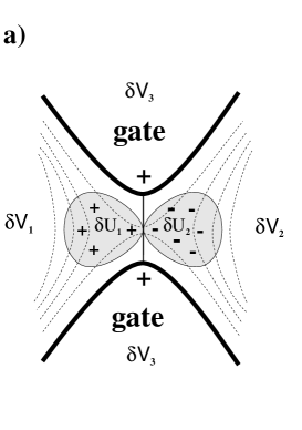
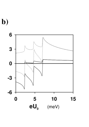
Figure 4.  : a) Quantum point contact with gates. The regions $\Omega_{1,2}$ at the left and right of the point contact can be charged. b) Capacitance $C_{\mu}$ and emittance $E_{11}$ of the QPC. Capacitances and emittances are in units of femto farads.

Assume a single open channel. Due to the symmetry of the problem, the geometric capacitance matrix can be written in the form

$${\bf C}=\left(\begin{array}[]{ccc}C_{0}+C&-C_{0}&-C\\ -C_{0}&C_{0}+C&-C\\ -C&-C&2C\end{array}\right)\;\;\;,$$ (51)

where $C_{0}$ is the geometric capacitance between $\Omega_{1}$ and $\Omega_{2}$ and where $C$ is the geometric capacitance between these regions and the gates. The electrochemical capacitance has again the form (48), with $C_{\mu}$ equal to the electrochemical capacitance across the QPC and with $C_{g}$ being the electrochemical gate capacitance. With the help of Eq. (17) and the characteristic potentials $u_{k\beta}=(D_{k\beta}-C_{\mu,k\beta})/D_{k}$ one finds

$$C_{g} = \frac{1}{C^{-1}+(D/2)^{-1}}$$ (52)

$$C_{\mu} = \frac{RC_{0}+(C/2)(1+R)+2C_{0}C_{g}D^{-1}}{1+2(2C_{0}+C)D^{-1}}\;\;.$$ (53)

The emittance elements (14) become

$$E_{11} = E_{22}=RC_{\mu}-DT^{2}/4+C_{g}T/2$$

$$E_{12} = E_{21}=C_{g}-E_{11}$$

$$E_{13} = E_{31}=E_{23}=E_{32}=-E_{33}/2=-C_{g}$$ (54)

with $D=2D_{1}$. The charge difference $\Delta q$ and the electrostatic voltage drop $\Delta U=\delta U_{1}-\delta U_{2}$ across the QPC are, respectively, given by

$$\frac{\Delta q}{\Delta V} = \frac{DR(2C_{0}+C)}{D+2(2C_{0}+C)}\;\;,$$ (55)

$$\frac{\Delta U}{\Delta V} = \frac{DR}{D+2(2C_{0}+C)}\;\;.$$ (56)

The discussion in the previous section is a limiting case of the general results given here. In the limit $C_{0}\to 0$ we obtain the results discussed for the quantum wire with a barrier collected in column three of table 1. In the limit $C\to 0$ overall charging of the QPC is prohibitive. The charge distribution is dipolar and the results of column $1$ of table 1 apply. In the limit $C\to\infty$ (corresponding to a geometrical capacitance of the QPC to the gates which is much larger than the capacitance across the QPC) an electrostatic voltage difference across the QPC does not develop, even so a charge imbalance exists. The results for this limiting case are collected in the middle column of table 1.
To generalize these results to the many channel case, we mention that for the potential considered the contributions of each individual channel just add. Each occupied subband $j$ contributes with a transmission probability $T^{(j)}$ to the total transmission function ${\cal T}$ $(=T_{11})=$ $\sum_{j}T^{(j)}$. The dc-conductance (3) is then given by $G_{11}^{(0)}=G_{22}^{(0)}=-G_{12}^{(0)}=-G_{21}^{(0)}=(2e^{2}/h){\cal T}$. Clearly, $G_{\alpha\beta}^{(0)}$ vanishes whenever one of the indices corresponds to the gate index $3$. Similarly the local PDOS (41) $D_{k}^{(j)}$ of each individual channel simply add. Hence, the local DOS becomes $D_{k}=\sum_{j}D_{k}^{(j)}$, and $T=1-R$ is now an average transmission probability defined by $T\equiv T_{k}=D_{k}^{-1}\sum_{j}D_{k}^{(j)}T^{(j)}$ where ($k=1,2$). Note that the average transmission probability $T$ ($\neq{\cal T}$) has nothing to do with the dc-conductance. If only a few channels are open the potential of the QPC has the from of a saddle point [42]. As a specific example we consider a quadratic potential $U(x)=U_{0}(b^{2}-x^{2})/b^{2}$ if $|x|\leq b$, and $U(x)=0$ if $b<|x|\leq l$. The transmission probabilities $T^{(j)}$ and the PDOS can be calculated analytically from a semiclassical analysis [43]. For simplicity, we assume a constant electrostatic capacitance $C_{0}=1\>fF$ between $\Omega_{1}$ and $\Omega_{2}$ and a fixed number of occupied channels in these regions. Both the height $U_{0}$ and the spatial variation of the potential should in principle be found by minimizing the grandcanonical potential for the system [44]. Here we consider $U_{0}$ as an independent control parameter. We assume that no additional channels enter into the regions $\Omega_{k}$ during the variation of $U_{0}$. In Fig. 4b. we show the results for a constriction with $b=500\>nm$, $l=550\>nm$, and with three equidistant channels separated by $E_{F}/3=7/3\>meV$. The dotted curve represents the transmission function which determines the dc conductance. At each step a channel is closed. The dashed and solid curves correspond to a gate with coupling $C=0$ and $C=C_{0}$, respectively. The curves represent the capacitance $C_{\mu}$ and the emittance $E_{11}$. For the two-terminal QPC ($C=0$) the capacitance vanishes and the emittance is negative for small $U_{0}$ where all channels are open. At each conductance step, the capacitance and the emittance increase and eventually merge when all channels are closed. Due to a weak logarithmic divergence of the WKB density of states at particle energies $E=eU_{0}$ (where WKB is not appropriate), the emittance shows steep edges between the steps. In the presence of the gate ($C\neq 0$), the curves are shifted upwards due to a capacitive contribution of the gate.

3.3 The resonant tunneling barrier

In the framework of the single-potential approximation introduced in Sect. 2.7 we discuss now the fully nonlinear $I$-$V$ characteristic and the fully frequency-dependent admittance of a resonant tunneling barrier (RTB) with a single resonant level. For a comparison of the results of our Hartree-like discussion (which to be realistic needs to be extended to a many level, many channel RTB) with theories that treat single electron effects, we refer the reader to the works by Bruder and Schöller [45], Hettler and Schöller [46], Stafford and Wingreen [47] and Stafford [48]. Consider the RTB sketched in Fig. 5a, where two reservoirs are coupled by a double barrier structure. The well between the barriers is considered to be the single relevant region. Additionally, the well may couple electrically with a capacitance $C$ to an external gate. We label quantities associated with the well with an index $0$. The band bottom of the well between the barriers and the energy of the resonant level are denoted by $eU_{0}$ and by $E_{0}=eU_{0}+E_{r}$, respectively. The electrochemical potentials of the particles which are scattered at the RTB are assumed to be close to the resonant level, such that the energy dependence of the scattering properties is described by a Breit-Wigner resonance with a width $\Gamma$. The asymmetry of the barrier is denoted by $\Delta\Gamma=\Gamma_{1}-\Gamma_{2}$, where $\Gamma_{\alpha}/\hbar$ is the escape rate of a particle trapped in the well through the barrier $\alpha$ . The scattering matrix elements have then a pole associated with a denominator $\Delta(E)=E-E_{0}+i\Gamma/2$,

$$s_{\alpha\beta}=e^{i(\varphi_{\alpha}+\varphi_{\beta})}\left(\delta_{\alpha\beta}-i\frac{\sqrt{\Gamma_{\alpha}\Gamma_{\beta}}}{\Delta(E)}\right)\;\;.$$ (57)

Here, the $\varphi_{\alpha}$ are arbitrary phases. We assume that the only energy dependence occurs in the resonant denominator, while the $\Gamma_{\alpha}$ and the $\varphi_{\alpha}$ are energy independent. One finds a transmission probability

$$T(E)=1-R(E)=\frac{\Gamma_{1}\Gamma_{2}}{|\Delta(E)|^{2}}$$ (58)

with a maximum value $T_{max}=4\Gamma_{1}\Gamma_{2}/\Gamma^{2}$. The injectivities and emissivities are equal to each other due to the absence of a magnetic field and are

$$D_{0\alpha}(E)=D_{\alpha 0}(E)=\frac{e^{2}}{2\pi}\>\frac{\Gamma_{\alpha}}{|\Delta(E)|^{2}}\;\;.$$ (59)

Summing up injectivities (or emissivities) yields the total DOS in the well

$$D_{0}=e^{2}\Gamma/2\pi|\Delta(E)|^{2}\;\;.$$ (60)

Again, the (P)DOS are here represented in units of a capacitance.

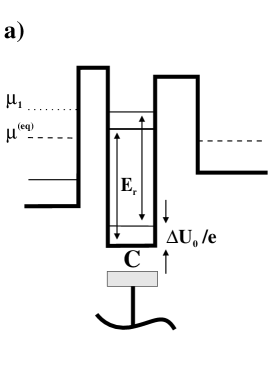
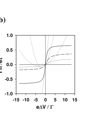
Figure 5.  : a) Resonant tunneling barrier with a single level and biased by voltages $V_{1}=(\mu_{1}-\mu^{(eq)})/e$ and $V_{2}=0$. The well may be coupled capacitively with a capacitance $C$ to a gate (dark region). b) Nonlinear current-voltage characteristic with $\Gamma_{1}=0.5$ meV, $\Gamma_{2}=1$ meV, $\Delta E=0$ (solid), $\Delta E=-\Gamma$ (dashed), $\Delta E=-2\Gamma$ (dotted). Thin dotted lines indicate the quadratic approximation.

Nonlinear transport

Let us discuss the nonlinear $I$-$V$ characteristic [2] for the charge neutral case ($C=0$). Note that only the effect of the resonant level is considered and that transport is still phase coherent. First, we determine the self-consistent potential. The relation between the electrostatic potential shift $\Delta U_{0}\equiv U_{0}-U_{0}^{(eq)}$ and the voltage shifts $V_{\alpha}=(\mu_{\alpha}-\mu^{(eq)})/e$ is obtained from the charge-neutrality condition

$$\int_{-\infty}^{\mu_{1}}D_{01}(E,U_{0})\>dE+\int_{-\infty}^{\mu_{2}}D_{02}(E,U_{0})\>dE-\int_{-\infty}^{\mu^{(eq)}}D_{0}(E,U_{0}^{(eq)})\>dE\equiv 0\;\;,$$ (61)

which can be integrated analytically. The result can be written as a function which determines implicitly $W\equiv\Delta U_{0}-(V_{1}+V_{2})/2$ as a function of $\Delta V$ only,

$$\Gamma\>{\rm arctan}[\frac{\Delta E}{\Gamma/2}] = \Gamma_{1}\>{\rm arctan}[\frac{\Delta E-e(W-\Delta V/2)}{\Gamma/2}]$$ (62)

$$+ \Gamma_{2}\>{\rm arctan}[\frac{\Delta E-e(W+\Delta V/2)}{\Gamma/2}]\;\;.$$

Equation (2) yields for the current $I\equiv I_{1}=-I_{2}$

$$I = \frac{2e}{h}\frac{\Gamma_{1}\Gamma_{2}}{\Gamma}\biggl{(}{\rm arctan}[\frac{\Delta E-e(W-\Delta V/2)}{\Gamma/2}]$$ (63)

$$- {\rm arctan}[\frac{\Delta E-e(W+\Delta V/2)}{\Gamma/2}]\biggr{)}\;\;,$$

where $\Delta E=\mu^{(eq)}-(eU_{0}^{(eq)}+E_{r})$ is the equilibrium distance between the Fermi energy and the resonance [2]. Without taking into account the self-consistent shift $\Delta U_{0}$ one would get a wrong result which is not gauge invariant. The current given by Eq. (63) saturates at a maximum value proportional to $\pi/2-{\rm arctan}(2\Delta E/\Gamma)$. The conduction is optimal for $\Delta E=0$ and $\Gamma_{1}=\Gamma_{2}$ when $I=(e/h)\Gamma{\rm arctan}(e\Delta V/\Gamma)$. In Fig. 5b we have plotted the characteristic for an asymmetry $\Delta\Gamma/\Gamma=-1/3$ and for various values of $\Delta E$. Due to the complete screening, the resonant level floates up or down to keep the charge in the well constant. An expansion of the current yields [2] $G_{111}^{(0)}=-(e^{3}/h)(\Delta\Gamma/2\Gamma)\partial_{E}T$ (thin dotted lines in Fig. 5b). The case of incomplete screening can similarly be treated with our approach. At large voltages, the resonance can then eventually fall below the conductance band bottom of the injecting reservoir as is known from semiconductor double-barrier structures. Finally we mention that, in general, even an elastically symmetric resonance can be rectifying if screening is asymmetric.

AC-Response

In order to calculate the admittances (28) we must know the external response $G_{\alpha\beta}^{e}$ defined for fixed potential. Using the specific scattering matrix elements (57), Eq. (26) gives

$$G^{e}_{\alpha\beta}(\omega)= \frac{e^{2}}{h}\int dE\>\frac{f(E)-f(E+\hbar\omega)}{\hbar\omega}\left(\delta_{\alpha\beta}-s_{\alpha\beta}^{\dagger}(E)s_{\alpha\beta}(E+\hbar\omega)\right)$$ (64)

$$=a_{\alpha\beta}\;g_{I}(\omega)$$

with

$$a_{\alpha\beta}(\omega)=\frac{4}{\Gamma(\hbar\omega+i\Gamma)}\left(\begin{array}[]{cc}\Gamma_{1}(\hbar\omega+i\Gamma_{2})&-i\Gamma_{1}\Gamma_{2}\\ -i\Gamma_{1}\Gamma_{2}&\Gamma_{2}(\hbar\omega+i\Gamma_{1})\end{array}\right)$$ (65)

and where

$$g^{I}(\omega)=\frac{e^{2}}{h}\frac{i\Gamma}{4}\int dE\>\frac{f(E)-f(E+\hbar\omega)}{\hbar\omega}\left(\frac{1}{\Delta(E+\hbar\omega)}-\frac{1}{\Delta^{\ast}(E)}\right)\;\;.$$ (66)

Here, we used

$$\frac{1}{\Delta(E+\hbar\omega)\Delta^{\ast}(E)}=\frac{1}{\hbar\omega+i\Gamma}\left(\frac{1}{\Delta(E+\hbar\omega)}-\frac{1}{\Delta^{\ast}(E)}\right)\;\;.$$ (67)

It turns out that $g^{I}(\omega)$ is the ac-admittance for the symmetric barrier without gate ($C=0$). This is is readily verified since for $C=0$ and for $a_{11}=a_{22}$ it holds

$$G(\omega)\equiv G^{I}_{11}(\omega)=\frac{G^{e}_{11}G^{e}_{22}-(G^{e}_{12})^{2}}{G^{e}_{11}+2G^{e}_{12}+G^{e}_{22}}=T_{max}\>g^{I}(\omega)\;\;.$$ (68)

In the case of $C=0$ it is thus sufficient to discuss the symmetric barrier. We consider first this case and assume zero temperature. The integral over the difference of the Fermi functions reduces then to a simple integral from $\mu^{(eq)}-\hbar\omega$ to $\mu^{(eq)}$ and can be carried out analytically. We find for the real part and the imaginary part of the admittance

$${\rm Re}[g^{I}(\omega)] = \frac{e^{2}}{h}\>\frac{\Gamma}{4\hbar\omega}\left(\arctan(\frac{\Delta E+\hbar\omega}{(\Gamma/2)})-\arctan(\frac{\Delta E-\hbar\omega}{(\Gamma/2)})\right)$$ (69)

$${\rm Im}[g^{I}(\omega)] = \frac{e^{2}}{h}\>\frac{\Gamma}{4\hbar\omega}\ln\sqrt{\frac{(|\Delta|^{2}-(\hbar\omega)^{2})^{2}+(\Gamma\hbar\omega)^{2}}{|\Delta|^{2}}}$$ (70)

where $|\Delta|\equiv|\Delta(\mu^{(eq)})|$. Our results for $g^{I}(\omega)$ are equivalent to earlier results of Fu and Dudley [6]. However, these authors neglect Coulomb interaction and, coincidentally, for a symmetric RTB, obtain the right expression only since they apply an antisymmetric bias $\pm\Delta V/2$ at the contacts.
An expansion of ${\rm Re}[G(\omega)]$ and ${\rm Im}[G(\omega)]$ with respect to frequency yields the coefficients defined in Eq. (6)

$$G^{(0)} = \frac{e^{2}}{h}T(E_{F})\;\;,$$ (71)

$$E = T_{max}\>\frac{D_{0}}{4}\left(\frac{|\Delta|^{2}-\Gamma^{2}/2}{|\Delta|^{2}}\right)\;\;,$$ (72)

$$K = \>\frac{he^{2}T(E_{F})}{(2\pi|\Delta|)^{2}}\left(\frac{|\Delta|^{2}-\Gamma^{2}/3}{|\Delta|^{2}}\right)\;\;.$$ (73)

We see, that $E$ and $K$ change sign. In particular, for the symmetric case this occurs if the value of the transmission probability $T$ equals $1/2$ and $3/4$, respectively. In Fig. 6a we plotted the real part and the imaginary part of the normalized admittance $g^{I}(\omega)/g^{I}(0)$ as a function of $\hbar\omega/|\Delta|$ for three different cases $T=1$ (solid), $T=0.5625$ (dashed), and $T=0.25$ (dotted). For $T<3/4$ there is a peak in the conductance which belongs to the excitation of the resonance by an energy quantum $\hbar\omega\approx|\Delta|$. We mention that the normalized admittance is determined by a single parameter $\gamma=\Gamma/|\Delta|$.

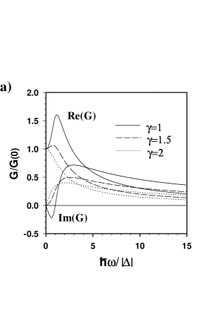
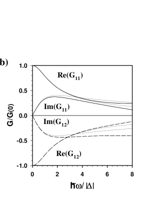
Figure 6.  : Frequency dependent admittance of the symmetric RTB. a) charge neutral ($C=0$) case, $\gamma=\Gamma/|\Delta|$; b) Influence of a weak gate: $G_{11}$ (solid) and $G_{12}$ (dashed) for $C|\Delta|/e^{2}=0.01$, $T=1$ (dotted: $C=0$).

We discuss now the effect of the capacitance $C$. In principle, by using the Eqs. (64) it is possible to derive expressions for the conductances (28). Here, we do not display the lengthy formulas but we rather present the results in a figure. A comparison of the admittance for $C=0$ (thin dotted curves) and for finite $C$ (thick curves) is shown in Fig. 6b for the resonant case $T=1$. One sees that for the small-capacitance case shown in the figure the Coulomb-coupling to the external gate enhances the capacitive part of the admittance. Indeed, an expansion with respect to the capacitance yields

$$G_{\alpha\beta}^{I}(\omega)=(-1)^{\alpha+\beta}G(\omega)-i\omega C\frac{\Gamma_{\alpha}\Gamma_{\beta}}{\Gamma^{2}}+{\cal O}(C^{2})\;\;.$$ (74)

In particular, one concludes $\sum_{\alpha\beta}G_{\alpha\beta}=-i\omega C+{\cal O}(C^{2})$ which follows also directly from the fact that the admittance $\sum_{\alpha\beta}G_{\alpha\beta}^{I}$ can be understood as a resistor (with an external admittance $\sum_{\alpha\beta}G_{\alpha\beta}^{e}$) in series with a capacitor (with a capacitance $C$).

The characteristic time-scales of tunneling problems [49] are a subject of considerable interest. With the analysis given above we are now able to identify characteristic times for the electric problem. We remark that the electrical problem investigated here leads to answers not for single electron motion, but for the collective charge dynamics. Consider the case of a RTB in the zero capacitance limit. From the expansion of the conductance up to quadratic order in frequency we can identify two characteristic frequencies or time-scales. There exists a frequency $\omega_{1}$ at which the magnitude of the dc-current and the displacement current are equal. The frequency $\omega_{1}$ is thus determined by $\tau_{1}=|E|/G^{0}$, where $E$ is the emittance and $G^{0}$ the dc-conductance. The time-scale $\tau_{1}$ is thus a generalization of the $RC$-time. For the RTB we find that this time is equal to $\tau_{1}=\hbar/\Gamma$ at resoance and is also equal to $\tau_{1}=\hbar/\Gamma$ far away from resonance. It vanishes for a Fermi energy at which the transmission of a symmetric barrier is equal to $1/2$. A second characteristic frequency is obtained by comparing the displacement current determined by the emittance $E$ with the second order dissipative term $K$. The second characteristic time $\tau_{2}$ is thus determined by $\tau_{2}=|K|/|E|$. At resonance this time is given by $\tau_{2}=(1/3)(\hbar/\Gamma)$. This time tends to zero for Fermi energies far away from resonance. It is singular at the Fermi energies at which the emittance vanishes and it is zero at the Fermi energies for which $K$ is zero. We conclude by mentioning that for the case in which the capacitance is not zero, the above consideration has to be applied to each element of the admittance matrix separately. In analogy to the tunneling time problem, where there exist characteristic times for traversal and reflection, from left and from right, the electrical problem will then be characterized by a set of characteristic frequencies or time scales for each admittance element, related only by sum rules due to current conservation and gauge invariance.

4 Conclusion

In this work we presented a theory for the admittance and the nonlinear transport of open (i.e. connected to different reservoirs) mesoscopic conductors. We have emphasized the application of this theory to a number of systems of current interest, like quantum wires, quantum point contacts, and resonant tunneling barriers. Our emphasis has been to derive results, which even so they might not be realistic in detail, nevertheless capture the essential physics. Our results should be useful both for comparison with additional theoretical work and with experimental work.

Due to the limitations of space, we have not reviewed a number of closely related subjects. The approach discussed here has been applied to ac-transport in two-dimensional electron gases in high magnetic fields [9, 38] which is particularly interesting in the regime where transport is dominated by carrier motion along edge states and by charging and de-charging of edge states. Of fundamental interest are Aharonov-Bohm effects in capacitance coefficients if one of the capacitor plates has the form of a ring [50] or for rings between capacitor plates [51]. As in dc-transport these interference effects are closely related to the sample specific fluctuations away from an average behavior. For a chaotic cavity capacitance fluctuations away from an ensemble averaged capacitance have been investigated by Gopar and Mello and one of the authors [52]. The ac-response and its fluctuations of a chaotic cavity connected to two leads and coupled capacitively to a back gate has been investigated by Brouwer and one of the authors. This system is particularly interesting since the ensemble averaged quantities exhibit weak localization corrections [53]. Since the weak-localization effect is not associated with a net charge accumulation the ac-response exhibits in addition to a Coulomb charge relaxation pole also a pole for uncharged excitations. Schöller [54] has investigated the dynamic capacitance of a one-dimensional wire. The dynamic capacitance exhibits interesting structure due to the plasma-modes of the one-dimensional wire. This list illustrates that there are many avenues to extend the work presented here. The application of the theory to more realistic models is a quite challenging undertaking but very likely also full of rewards.

Acknowledgments

This work was supported by the Swiss National Science Foundation under grant Nr. 43966.

Reference

This work is to be published in ”Mesoscopic Electron Transport”, edited by L. Kowenhoven, G. Schoen and L. Sohn, NATO ASI Series E, (Kluwer Ac. Publ., Dordrecht).

References

- [1] Büttiker, M., (1993) J. Phys.: Condens. Matter 5, 9631.
- [2] Christen, T., and Büttiker, M., (1996) Europhys. Lett. 35, 523.
- [3] Jackson, J. D, (1996) Am. J. of Physics 64, 855.
- [4] Büttiker, M., Thomas, H., and Prêtre, A., (1993) Phys. Rev. Lett. 70, 4114; Prêtre, A., Thomas, H., and Büttiker, M., (1996) Phys. Rev. B, Oct.
- [5] Pastawski, H., (1992) Phys. Rev. B46, 4053.
- [6] Fu, Y. and Dudley, S. C., (1993) Phys. Rev. Lett. 71, 466.
- [7] Büttiker, M., Thomas, H., and Prêtre, A., (1994) Z. Phys. B 94, 133.
- [8] Büttiker, M., (1995) in ”Quantum Dynamics and Submicron Structures”, edited by H. Cerdeira, G. Schön, and B. Kramer, (Kluwer Academic Publishers, Dordrecht) p. 657 -672.
- [9] Christen, T., and Büttiker, M., (1996) Phys. Rev. B 53, 2064.
- [10] Christen, T., and Büttiker, M., (1996) Phys. Rev. Lett. 76, 143.
- [11] Imry, Y., (1986) in Directions in Condensed Matter Physics, edited by G. Grinstein and G. Mazenko, (World Scientific Singapore) p. 101.
- [12] Beenakker, C. W. J., and van Houten, H., (1991) Quantum transport in semiconductor nanostructures, edited by. H. Ehrenreich and D. Turnbull (New York Academic Press).
- [13] Buot, F. A., Phys. Rep. (1993) 234, 73.
- [14] Datta, S., (1993) Electronic Transport in Mesoscopic Conductors, Cambridge University Press, 1995; Buot, F. A., Phys. Rep. 234, 73.
- [15] Landauer, R., (1970) Philos. Mag. 21, 863.
- [16] Büttiker, M., (1986a) Phys. Rev. Lett. 57, 1761.
- [17] Büttiker, M., (1988b) IBM J. Res. Develop. 32, 317.
- [18] Landauer, R., (1957) IBM J. Res. Develop. 1, 223.
- [19] Frenkel, J., (1930) Phys. Rev. 36, 1604.
- [20] Levinson, I. B., (1989) Sov. Phys. JETP 68, 1257.
- [21] Chen, W., Smith, T. P., Büttiker, M., and Shayegan, M., (1994) Phys. Rev. Lett. 73, 146.
- [22] Sommerfeld, P. K. H., van der Heijden, R. W., and Peeters, F. M., (1996) Phys. Rev. B 53, 13250.
- [23] Field, M., et al., (1996) Phys. Rev. Lett. 77, 350.
- [24] Pieper, J. B. and Price, J. C., (1994) Phys. Rev. Lett. 72, 3586.
- [25] Kouwenhoven, L. P., et al., (1994) Phys. Rev. Lett. 73, 3443.
- [26] Reznikov, M., Heiblum, M., Shtrikman, H., and Mahalu, D., (1995) Phys. Rev. Lett. 75, 3340.
- [27] Hofbeck, K., Genzer, J., Schomburg, E., Ignatov, A. A., Renk, K. F., Pavel’ev, D. G., Koschurinov, Yu., Melzer, B., Ivanov, S. Schaposchnikov, S., Kop’ev, P. S., (1996) Phys. Lett. A218, 349.
- [28] Taboryski, R., et al., (1994) Phys. Rev. B 49, 7813.
- [29] Glazman, L. I., and Khaetskii, A. V., (1989) Europhys. Lett. 9, 263.
- [30] Patel, N. K., et al., (1990) J. Phys.: Condens. Matter 2, 7247.
- [31] Kouwenhoven, L. P., et al., (1989) Phys. Rev. B 39, 8040.
- [32] Kluksdahl, N. C., et al., (1989) Phys. Rev. B 39, 7720.
- [33] Büttiker, M., and Christen, T., (1996) in Quantum Transport in Semiconductor Submicron Structures, edited by B. Kramer, (Kluwer Academic Publishers,Dordrecht); NATO ASI Series, Vol. 326, 263 -291.
- [34] Büttiker, M., Imry, Y., Landauer R., and Pinhas, S., (1985) Phys. Rev. B 31, 6207.
- [35] Büttiker, M., (1992b) Phys. Rev. B 46, 12485.
- [36] Gasparian, V. M., Christen, T., and Büttiker, M., (1996) Phys. Rev. A Oct.
- [37] Büttiker, M., Prêtre, A., and Thomas, H., (1993) Phys. Lett. A 180, 364.
- [38] Büttiker, M., and Christen, T., (1996) Dynamic Conductance in Quantum Hall Systems, to appear in ‘The application of high magnetic fields in semiconductor physics’, edited by G. Landwehr, (unpublished). cond-mat/9607051
- [39] Büttiker, M., (1992) Phys. Rev. B 45, 3807.
- [40] van Wees, B. J., et al., (1988) Phys. Rev. Lett. 60, 848.
- [41] Wharam, D. A., et al., (1988) J. Phys. C: Solid State Phys. 21, L209.
- [42] M. Büttiker, Phys. Rev. B 41, 7906 (1990).
- [43] Miller, S. C., and Good, R. M., (1953) Phys. Rev. 91, 174.
- [44] Chklovskii, D. B., Shklovskii, B. I., and Glazman, L. I., (1992) Phys. Rev. B 46, 4026.
- [45] Bruder, C., and Schöller, H., (1994) Phys. Rev. Lett. 72, 1076.
- [46] Hettler, M. H., and Schoeller, H., (1995) Phys. Rev. Lett. 74, 4907.
- [47] Stafford, C. A., and Wingreen, N. S., (1996) Phys. Rev. Lett. 76, 1916.
- [48] Stafford, C. A., (1996) Phys. Rev. Lett. 77, 2770.
- [49] Landauer, R., and Martin, Th., (1994) Rev. Mod. Physics 66, 217.
- [50] Büttiker, M., (1994) Physica Scripta, T 54, 104.
- [51] Büttiker, M. and Stafford, C. A., (1996) Phys. Rev. Lett. 76, 495.
- [52] Gopar, V. A., Mello, P. A., and Büttiker, M., (1996) Phys. Rev. Lett. 77 3005.
- [53] Brouwer, P. W., and Büttiker, M., (unpublished).
- [54] Schöller, H., (1996) (unpublished correspondence).