Mean field analysis of a model for superconductivity in an antiferromagnetic background

Abstract

We study a lattice fermion model for superconductivity in the presence of an antiferromagnetic background, described as a fixed external staggered magnetic field. We discuss the possibility that our model provides an effective description of coexistence of antiferromagnetic correlations and superconductivity, and its possible application to high temperature superconductivity. We also argue that, under certain conditions, this model describes a variant of the periodic Anderson model for heavy fermions. Using a path integral formulation we construct mean field equations, which we study in some detail. We evaluate the superconducting critical temperature and show that it is strongly enhanced by antiferromagnetic order. We also evaluate the superconducting gap, the superconducting density of states, and the tunneling conductivity, and show that the most stable channel usually has a $d_{x^{2}-y^{2}}$-wave gap.

I Introduction

Motivated by heavy–fermion– and high–temperature superconductors, considerable theoretical effort has gone into explaining the occurrence of unconventional superconductivity in strongly correlated electron systems. A basic model of interest here is the one-band Hubbard model which describes lattice fermions interacting with a strong on–site Coulomb repulsion [1]. This model is a widely studied candidate for explaining the unusual properties of the high temperature superconductors. Despite massive efforts this model is not yet well understood due to the technical difficulties involved. It is thus desirable to devise approximate simplified models focusing on certain aspects of the physics, that are easier to analyze than the full model, and whose properties can be compared with experiments and simulations. In this paper we study such a model focusing on the possible influence of antiferromagnetism on superconductivity.

There are several reasons for studying the coupling between antiferromagnetic (AF) correlations and superconductivity (SC): (i) The half filled Hubbard model is known to be an insulating antiferromagnet, and quantum Monte Carlo results [1] and results from Hartree-Fock theory [2] indicate that local AF correlations persist up to quite high doping levels (at least for parameters adequate for high temperature superconductivity). (ii) The parent compounds of the high-temperature superconductors (HTSC) are Mott insulators with antiferromagnetic long range order. Neutron scattering experiments [3] show that the antiferromagnetic correlation length gets reduced upon doping. NMR measurements, however, suggest that strong short range AF correlations remain important all the way into the SC phase (see Ref. [4] for a recent discussion on this point). (iii) As we will further discuss below, AF correlations may also play a role in the periodic Anderson model for heavy fermions [5]. (iv) Finally there are other (low–$T_{c}$) superconductors which exhibit simultaneous SC and AF order [6, 7].

Several different approaches to consider the effects of AF correlations on HTSC have been explored in the literature. One frequently studied model is based on fermion pairing due to exchange of AF spin fluctuations [8]. Another is the spin bag mechanism which is based on the idea that local suppression of the AF gap leads to an effective attraction between certain quasiparticles, and thus to superconductivity [9]. Recently Dagotto and coworkers proposed and studied weak coupling models of holes in an antiferromagnet, using a numerically determined dispersion relation [10]. Most of these models lead to $d_{x^{2}-y^{2}}$ pairing, which indeed seems to be observed in experiments on HTSC [11].

The model studied in this paper describes lattice fermions in an external antiferromagnetic field coupled to the fermion spin. We also include various attractive, instantaneous fermion-fermion couplings (see Sec. II A). Although we use a field with AF long-range order, we argue below that, for the properties we calculate, this model gives a good approximation also when the AF order parameter is slowly varying in the sense further discussed below. Our model illustrates in a simple way how correlations can narrow the quasiparticle bands which increases the density of states (DOS) and hence increases $T_{c}$ [12, 13]. This is an example of the van Hove scenario which has been frequently discussed in the context of HTSC [14, 10]. In our model the enhancement of the van Hove singularity by antiferromagnetism increases $T_{c}$, such that the right order of magnitude for HTSC can be obtained by reasonably small couplings. Recent numerical results suggest that in the parameter range of interest for HTSC, the Hubbard model has a DOS peak, and the chemical potential intersects this peak for certain finite doping [15]. While it is clear that the simple band structure obtained in our model is not going to be realistic in detail, our model attempts to (i) represent the states at this peak by the AF bands, and (ii) to model the resulting superconducting properties. Since our model is simple, our investigation can be done in some detail which would be difficult for more realistic models. Our approach is similar to Ref. [10] in that we attempt to model quasiparticle bands renormalized by strong correlations and then investigate their superconducting properties, but otherwise the models are quite different.

The model we study naturally leads to a superconducting gap $\Delta$ with a staggered real space structure (i.e., with a two component order parameter). A superconducting order parameter with such a structure has been studied previously on a phenomenological level in the context of heavy fermions [16]. Our results show how such an order parameter can arise in microscopic models.

The first purpose of this paper is to provide motivation for our model and develop efficient tools to study it. In any case, our model should describe systems where antiferromagnetic order and superconductivity coexist [7]. However, we also argue that it can be regarded as a useful toy model for studying the effects of band renormalization by strong correlations on superconductivity in HTSC or heavy fermion systems. The idea is that by using a Hubbard–Stratonovich transformation, an interacting fermion systems can be represented as non–interacting fermions coupled to a dynamical boson field. A simple approximation is to replace the dynamical boson field by a fixed boson field, which is determined by Hartree-Fock (HF) equations. A general feature of the doped Hubbard model is that this HF field has a nontrivial spatial dependence [2]. This leads to a variety of complicated bands. The model studied in this paper represents the simplest nontrivial case where this occurs. To study this model, we use an efficient path integral formalism which should be useful also in more complicated cases, and we derive mean field equations of BCS type. To further investigate the relevance of the description provided by our model a more elaborate analysis (e.g. fluctuation calculations) is required, but this is beyond the scope of this paper.

The second purpose of the paper is to calculate some physical properties of the model. Using parameters motivated by HTSC, we present a systematic analysis of the different possible SC channels. We study the effect of on–site, nearest neighbor (nn) and next–nearest neighbor (nnn) interactions. We find that the dominating channels are neither translation– nor spin rotation invariant. In the presence of AF correlations, we find that on-site attraction never leads to significant pairing and nn attraction is most efficient and usually produces a $d_{x^{2}-y^{2}}$-wave gap, ${\it\Delta}\propto\cos(k_{1})-\cos(k_{2})$. For dominant nnn-attraction we get $p$-wave pairing, ${\it\Delta}\propto\sin(k_{1}+k_{2})+\sin(k_{1}-k_{2})$. $d_{x^{2}-y^{2}}$-wave superconductivity has been found in numerous other calculations [11], but our result shows that it arises already in a particularly simple model. We also derive and solve the gap equations for nn coupling in the full temperature range below $T_{c}$. Our formalism is convenient to evaluate SC properties. As an example, we evaluate the SC density of states and the resulting tunneling conductance as a function of temperature. We note that some features of our results appear qualitatively similar to HTSC, e.g. the doping dependence of $T_{c}$ and the tunneling conductance.

The plan of this paper is as follows. In Section II we give a detailed description of the model, and then discuss the possibility that it may provide a simple description of certain aspects of the physics of the Hubbard model with an additional weak pairing interaction. We also relate our model to the periodic Anderson model for heavy fermions [5] Section II C. Our analysis of the model starts in Section III, where we summarize the path integral formalism. The mean field equations are obtained in Section IV. We first (Sec. IV B) obtain the $T_{c}$-equations for all possible superconducting channels (singlet, and triplet, translational-invariant and staggered, $s$-, $p$- and $d$-wave) which are needed in our systematic stability analysis, and then (Sec. IV C) derive the gap equations below $T_{c}$ for the dominating channels. Section V contains our numerical results of our stability analysis, the temperature dependence of the SC gap, and the density of states and the tunneling conductance as a function of $T<T_{c}$. We end with conclusions in Section VI. Some technical details are in two appendices.

II The model

In this section we present our model (A). We then discuss the relation of our model to the doped Hubbard model (B) and the periodic Anderson model (C).

A Model description

Our model Hamiltonian describes lattice fermions with field operators $a^{(+)}_{\uparrow,\downarrow}({\bf x})$ in an external staggered magnetic field ${\bf B}({\bf x})$ and an additional weak attractive BCS-like interaction,

$$H_{\rm eff}=H_{\rm hop}+\sum_{{\bf x}}{\bf S}({\bf x})\cdot{\bf B}({\bf x})\,e^{{i}{\bf Q}\cdot{\bf x}}+H_{\rm int}$$ (1)

where ${\bf B}=(B_{1},B_{2},B_{3})$ is the staggered magnetic field representing the AF order,

$$H_{\rm hop}=-\sum_{\langle{\bf x},{\bf y}\rangle,\sigma}t\,a^{+}_{\sigma}({\bf x})a_{\sigma}({\bf y})$$ (2)

is the usual hopping Hamiltonian (i.e. the sum over all nearest-neighboring sites $\langle{\bf x},{\bf y}\rangle$), ${\bf S}=a^{+}({\bf x}){\mbox{\boldmath$\sigma$}}a({\bf x})$ is 2 times the electron spin operator ($\sigma$ are the Pauli spin matrices), and

$$H_{\rm int}=\frac{1}{2}\sum_{{\bf x},{\bf y}}n({\bf x})V({\bf x}-{\bf y})n({\bf y}),\quad n=\sum_{\sigma}a_{\sigma}^{+}a_{\sigma}$$ (4)

is a (weak) attractive charge-charge interaction. We consider the model on a $d$-dimensional cubic lattice ${\mathbb{Z}}^{d}$ (i.e. spatial vectors are ${\bf x}=(x_{1},\ldots,x_{d})$ with $x_{i}$ integers), and ${\bf Q}=(\pi,\ldots,\pi)$ is the usual AF vector. We use a pairing potential with the Fourier transform

$$V({\bf k})=-g_{0}-g_{\rm nn}\sum_{i}2\cos(k_{i})-g_{\rm nnn}\sum_{i\neq j}2\cos(k_{i})\cos(k_{j})$$ (5)

where ${\bf k}=(k_{1},\ldots,k_{d})$ with $-\pi\leq k_{i}\leq\pi$ and $g_{i}>0$. The first, second and third terms here describe on-site, nearest neighbor (nn) and next-to-nearest neighbor (nnn) instantaneous interactions. We take the corresponding couplings $g_{i}$ as input parameters of our model. A useful way to think about this potential is as coming from a Taylor expansion of some general potential $V({\bf x}-{\bf y})$, where only the lowest order terms are kept since they are the only ones expected to be important for SC. Note that the normalization in Eq. (5) is such that $V({\bf x}-{\bf y})$ is $-g_{0}$, $-g_{\rm nn}$ and $-g_{\rm nnn}$ if ${\bf x}$ and ${\bf y}$ are equal, nn, and nnn, respectively. We do not fix dimension in our formal manipulations, but in our numerical calculations we take $d=2$.

We will analyze the model setting ${\bf B}({\bf x})$ independent of ${\bf x}$. This case is of interest for materials where AF long range order coexisting with SC has been observed [7, 6]. However, we expect that our results are also adequate for the case of varying staggered magnetic fields ${\bf B}({\bf x})$, as long as this variation is slow. Arguments for this will be given below. In particular, even though the second term in Eq. (1) explicitly breaks spin rotation invariance, this model can nevertheless describe also situations where this symmetry is unbroken: one can think of Eq. (1) as coming from an adiabatic approximation (similar to the Born–Oppenheimer approximation) of a strong–coupling model in which the dynamical AF fluctuations are frozen, and spin rotation invariance will be restored after averaging over certain ${\bf B}({\bf x})$–configurations.

B On the relation to the doped Hubbard model

Here we describe how our model can be related to the doped Hubbard model with an additional attractive interaction $H_{\rm int}$ as in Eq. (4). The idea is to replace the strong Coulomb interaction by coupling the fermions to dynamical bosons. In the path integral formalism this can be done by a Hubbard-Stratonovich transformation which introduces dynamical boson fields [17]

$$\phi_{0}(\tau,{\bf x})=r(\tau,{\bf x}),\quad\mbox{\boldmath$\phi$}(\tau,{\bf x})={\bf B}(\tau,{\bf x})\,e^{{i}{\bf Q}\cdot{\bf x}}$$ (6)

depending on imaginary time $\tau$. These fields have a simple physical interpretation: $s=|{\bf B}|$ and ${\bf e}={\bf B}/|{\bf B}|$ represent the magnitude and direction of the AF ordered fermion spins and $r$ the fermion charge.

A standard approximation then is to replace this dynamical boson fields by a fixed and static boson field configuration. This formally amounts to a saddle point evaluation of the exact boson path integral. The stationary points in this path integral are determined by HF equations, and this procedure corresponds to mean field theory. For the doped Hubbard model this approximation is already quite involved: Numerical results show that the HF solutions have a complicated spatial dependence and, depending on parameters, describe magnetic domain walls, magnetic vortices etc. [2]. However, in the parameter regime of interest all these solutions exhibit antiferromagnetic correlations. The non–trivial assumptions required to establish a connection of our model to the Hubbard model are (i) HF theory is adequate to determine interacting fermions bands, (ii) it is mainly these antiferromagnetic correlations which determine these bands close to the Fermi surface.

Let us be more specific on point (ii): For thin domain walls or localized vortices (e.g.), $r({\bf x})=r$ and ${\bf B}({\bf x})={\bf B}$ are constant in large regions of configuration space. Then there are fermion states which, for most ${\bf x}$, coincide with states describing a system with constant $r({\bf x})=r$ and ${\bf B}({\bf x})={\bf B}$. Theses states can be viewed as scattering solutions, e.g., in a domain wall background. Our model tries to capture the effect of AF correlations on such delocalized states. Our assumption is that such states exist and that for suitable doping, they are at the Fermi energy. Note that the filling $\rho$ used in our model should not be interpreted as filling in the Hubbard model: $\rho-1$ is the doping of the AF band, which is smaller than the total doping if part of the charge carriers are bound, e.g., in domain walls. A check of the properties we assumed requires a rather detailed analysis of the Hubbard model itself and is beyond the scope of this paper. These properties seem however to have some support from recent numerical simulation results for the Hubbard model, which indicate that for parameters adequate for HTSC, $\mu$ indeed intersects a peak in the DOS at a certain doping level [15].

We analyze the model setting ${\bf B}(x)$ independent of $x=(\tau,{\bf x})$, but we expect that our results are a good approximation also if ${\bf B}(x)$ varies slowly or only in small fractions of spacetime. Then the 2-point Green functions of our model can be approximated by

$$G(x,y)\approx G_{N}(x-y,y)+G_{A}(x-y,y)\,e^{{i}{\bf Q}\cdot{\bf y}}$$ (7)

where $G_{N,A}$ depends on the second argument $y$ only via ${\bf e}(y)\cdot\mbox{\boldmath$\sigma$}$ and $s(y)$. These Green functions can be obtained from the ones for ${\bf B}(y)=s\,{\bf e}=const$ in leading order of a gradient expansion. In particular, thermodynamic properties only depend on $s(y)$ in this approximation. If $s(y)\approx const$, we thus expect that the thermodynamic properties of our model should not depend much on the AF correlation length (assuming the latter is large enough). If $s(y)$ also varies in small fractions of spacetime, the thermodynamic properties are appropriate averages of the ‘local’ properties which can be deduced from the results in this paper.

C On the relation to the periodic Anderson model

Here we present an argument that our model, with constant ${\bf B}$, can be obtained from the periodic Anderson model in a certain parameter regime. The physical picture is as follows: the periodic Anderson model is a 3D lattice fermion model with two kinds of spin-$\frac{1}{2}$ fermions: $f$-electrons with a strong Hubbard repulsion are coupled weakly to non-interacting $a$-electrons [5]. For large on-site repulsion, the $f$-electrons can be regarded as half filled and antiferromagnetically ordered. The lower magnetic $f$-band is then far underneath the Fermi surface and the upper one far above. Thus the $f$-electrons are in a half–filled band and thus act as a commensurate [${\bf e}(x)=const$] AF background for the weakly coupled $a$-electrons, and our model provides an effective weak-coupling description of these $a$-electrons.

We now turn to a more detailed argument. We start from the following periodic Anderson Hamiltonian

$$H=H_{\rm hop}+H_{f}+V_{fa}+H_{\rm int}$$ (9)

where $H_{\rm hop}$ and $H_{\rm int}$ are as above, and

$$H_{f}=\sum_{{\bf x}}\Bigl{(}-\epsilon_{f}n_{f}({\bf x})+U\,n_{f,\uparrow}({\bf x})n_{f,\downarrow}({\bf x})\Bigr{)}$$ (10)

describes another species of electrons denoted as $f$ which are localized and have a strong on-site charge-charge repulsion $U>>\epsilon_{f}>>t$ ($n_{f,\sigma}({\bf x})=f_{\sigma}^{+}({\bf x})f_{\sigma}({\bf x})$, and $n_{f}=n_{f,\uparrow}+n_{f,\downarrow}$). The interaction of the $a$ and $f$ electrons is local,

$$V_{fa}=\lambda\sum_{{\bf x}}\Bigl{(}a^{+}_{\sigma}({\bf x})f_{\sigma}({\bf x})+f^{+}_{\sigma}({\bf x})a_{\sigma}({\bf x})\Bigr{)}\,,$$ (11)

and $H_{\rm int}$ is as in Eq. (4) i.e., we assume the BCS attraction among the $a$ electrons only. $H_{a}+H_{f}+V_{fa}$ is the Anderson Hamiltonian: $H_{f}$ is the usual strongly repulsive Hubbard Hamiltonian (with hopping constant $t_{f}\to 0$) which in the half-filled case (one $f$-electron per site) describes antiferromagnetically ordered electrons. The $a$-electrons are assumed in the conduction band weakly coupled to the $f$-electrons, and since $U>>\epsilon_{f}>>\lambda^{2}$ and $\epsilon_{f}>>t$, one still expects the $f$ electrons to form a half-filled antiferromagnet.

The simple physical picture leading to the effective Hamiltonian $H_{\rm eff}$ is that the coupling between the $f$ and $a$ electrons and the antiferromagnetic ordering of the former produces an effective staggered magnetic field that couples to the spin of the $a$ electrons. The staggered magnetic field ${\bf B}$ is determined by the interband coupling (see below). This effect is independent of the filling in the $a$ band, because the antiferromagnetism comes from the $f$ band, which is half-filled. This makes the situation simpler than in the non-half-filled repulsive Hubbard model, where commensurate order cannot be assumed.

In the remainder of this section, we derive $H_{\rm eff}$ from $H$ by an argument patterned after Anderson’s derivation of the Heisenberg antiferromagnet from the half-filled Hubbard model.

We do a second-order perturbation expansion in $\lambda$ to show that the coupling between the $a$ and the $f$ electrons produces the staggered field term of the effective Hamiltonian. For $\lambda=0$, the ground state wave function factors into the product of that of the ground state for the $a$ and the $f$. Since the $f$ system is half-filled because $U$ is large, the ground state wave function for the $f$ electrons is

$$|\ \hbox{N\'{e}el}\ \rangle=\prod\limits_{{\bf x}}f^{+}_{\sigma({\bf x})}({\bf x})|0\rangle\,,\quad\sigma({\bf x})=e^{{i}{\bf Q}\cdot{\bf x}}$$ (12)

where $|0\rangle$ denotes the empty state (and $\sigma({\bf x})$ means $\uparrow$ if $+1$ and $\downarrow$ otherwise). The Hilbert space of the total system is the sum of the two orthogonal subspaces ${\cal H}_{a}$ and ${\cal H}_{f}$. Correspondingly, the Hamiltonian has the matrix structure ($V_{fa}=\lambda V$ and $H_{a}=H_{\rm hop}+H_{\rm int}$)

$$H=\left(\matrix{H_{a}&V_{fa}\cr V_{fa}&H_{f}\cr}\right)=H_{0}+\left(\matrix{0&\lambda V\cr\lambda V&0\cr}\right)\,.$$ (13)

The potential term appears off-diagonal because it couples the two subspaces. The resolvent is also a matrix, and the resolvent equation

$$\frac{1}{E-H} = \frac{1}{E-H_{0}}+\frac{1}{E-H_{0}}\ V_{fa}\ \frac{1}{E-H}$$

$$= \frac{1}{E-H_{0}}+\frac{1}{E-H_{0}}\ V_{fa}\ \frac{1}{E-H_{0}}$$

$$+ \frac{1}{E-H_{0}}\ V_{fa}\ \frac{1}{E-H_{0}}\ V_{fa}\ \frac{1}{E-H}$$

reads, denoting $R_{a}=(E-H_{a})^{-1}$ and $R_{f}=(E-H_{f})^{-1}$,

$$\frac{1}{E-H} = \left(\matrix{R_{a}&0\cr 0&R_{f}\cr}\right)+\lambda\left(\matrix{0&R_{a}VR_{f}\cr R_{f}VR_{a}&0\cr}\right)$$ (14)

$$+ \lambda^{2}\left(\matrix{R_{a}VR_{f}V&0\cr 0&R_{f}VR_{a}V\cr}\right)\ \frac{1}{E-H}\,.$$ (16)

We want to calculate the effective propagation of the $a$ electrons to second order in $\lambda$. For this we need only the left upper element $R_{\rm eff}=\left(\frac{1}{E-H}\right)_{aa}$. It is given by

$$R_{\rm eff}=R_{a}+\lambda^{2}R_{a}VR_{f}VR_{\rm eff}$$ (17)

or in other words

$${R_{\rm eff}}^{-1}=E-H_{a}-\lambda^{2}VR_{f}V$$ (18)

Up to this point, everything was exact. Now we approximate by keeping only terms up to order $\lambda^{2}$. Moreover, since we want to see the influence of the interaction in the ground state only, we may calculate $VR_{f}V$ by its expectation with respect to $f$, taken in the state $|\ \hbox{N\'{e}el}\ \rangle$. This gives a staggered magnetic field term

$$\frac{1}{E+\epsilon_{f}+U}\sum_{{\bf x}}a^{+}({\bf x})\sigma_{3}a({\bf x})\,e^{{i}{\bf Q}\cdot{\bf x}}$$ (19)

Finally, we want to define the effective Hamiltonian $H_{\rm eff}$ by ${R_{\rm eff}}^{-1}=E-H_{\rm eff}$. To do so, we note that the energy $E$ is in the $a$ band, so $|E|\leq 2t<<\epsilon_{f}+U$, and thus we may replace $\frac{1}{E+\epsilon_{f}+U}$ by $\frac{1}{\epsilon_{f}+U}$. With this approximation, ${R_{\rm eff}}^{-1}$ depends only linearly on $E$, and, up to an uninteresting shift in the energy,

$$H_{\rm eff}=H_{a}+\frac{\lambda^{2}}{\epsilon_{f}+U}\sum_{{\bf x}}a^{+}({\bf x})\sigma_{3}a({\bf x})\,e^{{i}{\bf Q}\cdot{\bf x}}$$ (20)

is the effective Hamiltonian. Since $H_{\rm int}$ couples only the $a$ electrons, it does not play a role in this argument. The coupling also produces a feedback on the $f$ electrons, but this influences the $a$ electrons only in higher order in $\lambda$. This shows that a model of the type we study is induced, but the ${\bf B}$ field obtained by this argument is small.

III Formalism

A Functional integrals and mean field approximation

To study our effective model, we use the path integral formalism [18]. It is equivalent to the Hamiltonian framework and more convenient for calculating the grand canonical partition function $Z={\rm Tr}\,e^{-\beta(H-\mu N)}$, which is thus expressed as a functional integral $Z=\int{\cal D}\bar{\psi}{\cal D}\psi\,e^{-{\cal A}}$ over Grassmann variables $\psi_{\sigma}(x)$ and ${\bar{\psi}}_{\sigma}(x)$ carrying a spin index $\sigma=\{\uparrow,\downarrow\}$. Configuration space is labeled by $x=(\tau_{x},{\bf x})$ where $0<\tau_{x}<\beta$ is the usual imaginary time and ${\bf x}$ are vectors in the $d$-dimensional cubic lattice ${\mathbb{Z}}^{d}$ (i.e. we set the lattice constant equal to 1). Most of our calculations are for arbitrary $d$, but we are mainly interested in $d=2$ or $3$. In intermediate steps of our derivation we will implicitly assume that space is a finite square (cube) with a finite number $L^{d}$ of points, but we will eventually take the thermodynamic limit $L\to\infty$. We group the spacetime argument $x$ and the spin index $\sigma$ to a single coordinate $X=(x,\sigma)$, and set $\psi(X)=\psi_{\sigma}(x)$ etc. We also use convenient short hand notations $\sum_{x}\equiv\int_{0}^{\beta}d\tau_{x}\sum_{{\bf x}\in\Lambda}$ and $\sum_{X}=\sum_{x,\sigma}$ etc.

The action of the model is ${\cal A}=\sum_{X}\bar{\psi}(X)(\partial_{\tau}-\mu)\psi(X)+\int_{0}^{\beta}H(\bar{\psi},\psi)d\tau={\cal A}_{2}+{\cal A}_{4}$, with a quadratic part defining the free Green function, ${\cal A}_{2}=-\sum_{X,Y}\bar{\psi}(X){G_{0}}^{-1}(X,Y)\psi(Y)$, and a quartic interaction term.

To derive mean field equations for possible superconducting states we now introduce auxiliary bilocal pair fields and thus decouple the fermion interaction (see e.g. [19]),

$$e^{-{\cal A}_{4}}=\int{\cal D}\Delta^{*}{\cal D}\Delta\,\exp\sum_{X,Y}\Bigl{(}\frac{|\Delta(X,Y)|^{2}}{2V(X,Y)}$$ (21)

$$\nopagebreak-\frac{1}{2}\overline{\Delta(X,Y)}\psi(Y)\psi(X)-\frac{1}{2}\bar{\psi}(X)\bar{\psi}(Y)\Delta(X,Y)\Bigr{)}$$ (22)

where

$${\cal D}\Delta^{*}{\cal D}\Delta=\prod\limits_{\{X,Y\}}\frac{d{\rm Re}\Delta(X,Y)d{\rm Im}\Delta(X,Y)}{2\pi|V(X,Y)|}$$ (23)

is the measure for a complex boson path integral. The product runs only over those unordered pairs $\{X,Y\}$ for which $V(X,Y)\neq 0$. We call the $\Delta(X,Y)$ Hubbard-Stratonovich (HS) fields. Note that the integral over $\Delta(X,Y)$ is convergent because (and only if) the pairing potential is purely attractive, i.e. $V(X,Y)<0$ whenever it is nonzero. Note also that due to the anticommutativity of the Grassmann variables only antisymmetric configurations,

$$\Delta(X,Y)=-\Delta(Y,X)\,,$$ (24)

contribute to the path integral. This corresponds to the Pauli principle.

Integrating out the fermions now leads to

$$Z=\int{\cal D}\Delta^{*}{\cal D}\Delta\,e^{-{\cal F}(\Delta)}$$ (25)

with the effective HS action

$${\cal F}(\Delta)=-\sum_{X,Y}\frac{|\Delta(X,Y)|^{2}}{2V(X,Y)}-\frac{1}{2}{\rm Tr}\log({\cal G}^{-1})$$ (26)

where the second term come from the fermion path integral (logarithm of Pfaffian of ${\cal G}^{-1}$ = half of logarithm of determinant of ${\cal G}^{-1}$), and we have introduced

$${\cal G}^{-1}={\cal G}_{0}^{-1}-\Sigma$$ (27)

with

$${\cal G}_{0}=\left(\matrix{G_{0}&0\cr 0&\tilde{G_{0}}}\right),\quad\tilde{G_{0}}(X,Y)=-G_{0}(Y,X)$$ (28)

the free Nambu Green function and

$$\Sigma=\left(\matrix{0&\Delta\cr\Delta^{*}&0}\right),\quad\Delta^{*}(X,Y)=\overline{\Delta(Y,X)}\>.$$ (29)

In the following we write

$${\cal G}=\left(\matrix{G&F\cr F^{*}&\tilde{G}}\right)$$ (30)

which is equal to the Nambu Green function for non-interacting fermions in an external field $\Delta$.

HF theory amounts to evaluating the HS path integral in Eq. (25) using the saddle point method. We obtain $Z\approx\exp[-{\cal F}(\Delta_{HF})]$ where $\Delta_{HF}$ is the solution of the saddle point equation $\delta{\cal F}(\Delta)/\delta\Delta(X,Y)=0$ which corresponds to the minimum of ${\cal F}$. More explicitly the (complex conjugate of the) latter equation is

$$\Delta(X,Y)=V(X,Y)F(X,Y)$$ (31)

which together with Eq. (27) forms a self consistent system of equations and provides the BCS description for our model. Note that in the saddle–point approximation, $-\langle\Psi(X)\Psi(Y)^{\dagger}\rangle={\cal G}$, so Eq. (27) can now be interpreted as the Dyson equation for our electron Green function ${\cal G}$ where mean field theory gives the approximation (31) for the electron self energy $\Sigma$.

The general analysis of the mean field equations is still too difficult since for general $X,Y$ dependent HS field configurations $\Delta(X,Y)$, the evaluation of the Nambu Green function (30) is impossible in general. To proceed we therefore make the usual assumption and only consider HS configurations that have at least a remnant of translation invariance. Since for our model the free Green function contains a staggered contribution i.e. is not invariant under translations by one but only two sites, the simplest consistent ansatz for our HF equations are HS configurations $\Delta$ invariant by translations by two sites.

IV Staggered superconductivity

A Staggered states

We now specialize to time independent states where the superconducting order parameter has a uniform part and a staggered part, i.e. [20]

$$\Delta({\bf x},{\bf y})=\Delta_{N}({\bf x}-{\bf y})+\Delta_{A}({\bf x}-{\bf y})e^{i{\bf Q\cdot y}},$$ (32)

with ${\bf Q}=(\pi,\ldots,\pi)$ the antiferromagnetic vector (here and below we use spin matrix notation whenever possible). This obviously implies that ${\cal G}$ is also a sum of a uniform and staggered contribution, and we can solve the Dyson equation (27) by Fourier transformation. We use the convention

$\displaystyle f(x)=\sum_{k}e^{-{i}kx}f(k)\,,\quad kx=\omega_{n}\tau_{x}-{\bf x}\cdot{\bf k}$where $k=(\omega_{n},{\bf k})$ with $\omega_{n}=\frac{(2n+1)\pi}{\beta}$ ($n\in{\mathbb{Z}}$) the Matsubara frequencies and ${\bf k}=(k_{1},\ldots,k_{d})$ a momentum vector in the first Brillouin zone $[-\pi,\pi]^{d}$ of the lattice, i.e.

$\displaystyle\sum_{k}\equiv\frac{1}{\beta}\sum_{\omega_{n}}\int\!{\mkern 2.0mu\mathchar 22\relax\mkern-2.0mu\mkern-9.0mud}{\bf k}\,\,,\quad\int\!{\mkern 2.0mu\mathchar 22\relax\mkern-2.0mu\mkern-9.0mud}{\bf k}\,\equiv\int\limits_{[-\pi,\pi]^{d}}\frac{d^{d}{\bf k}}{(2\pi)^{d}}\,.$Then $f(k)=\sum_{x}e^{{i}kx}f(x)$.

With that the self-energy equation (31) becomes

$$\Delta_{N,A}(k)=\sum_{q}V(k-q)F_{N,A}(q)\,.$$ (33)

B $T_{c}$-equations

We first consider the region close to the critical temperature $T_{c}$ where the Dyson equation (27) can be linearized in the non-gauge invariant Green functions $F$ and self energy $\Delta$. Writing (27) as ${\cal G}={\cal G}_{0}+{\cal G}_{0}*\Sigma*{\cal G}_{0}+\cdots$ we obtain the linearized equation $F=G_{0}*\Delta*\tilde{G}_{0}$ i.e.

$$F(x,y)=\sum_{z_{1},z_{2}}G_{0}(x,z_{1})\Delta(z_{1},z_{2})\tilde{G}_{0}(z_{2},y)$$ (34)

where $\tilde{G}_{0}(x,y)\equiv-G_{0}(y,x)^{T}$ and ^T means matrix transposition. With the ansatz (32) and Fourier transform this becomes (the $k$ dependence is suppressed, $F_{N}\equiv F_{N}(k)$ etc., in the following),

$$F_{N,A}=G_{0N}\Delta_{N}\tilde{G}_{0N,A}+G_{0A}\Delta_{N}^{Q}\tilde{G}_{0A,N}^{Q}$$ (35)

$$\nopagebreak+G_{0A}\Delta_{A}^{Q}\tilde{G}_{0N,A}+G_{0N}\Delta_{A}\tilde{G}_{0A,N}^{Q}$$ (36)

where $\Delta_{N}^{Q}(k)=\Delta_{N}(k-Q)$ etc, and spin matrix multiplication is understood. Combined with Eq. (33), this gives the $T_{c}$ equations for our model.

The translation-invariant and staggered parts of the free Green function, $G_{0N,A}$ are

$$G_{0N}(k)=g(k)\sigma_{0},\quad G_{0A}(k)=a(k)\sigma_{3}$$ (38)

where

$$g(k)=\frac{{i}\omega_{n}+\mu+\epsilon({\bf k})}{({i}\omega_{n}-E_{+})({i}\omega_{n}-E_{-})}$$ (39)

$$\nopagebreak a(k)=\frac{{s}}{({i}\omega_{n}-E_{+})({i}\omega_{n}-E_{-})}$$ (40)

[we used $\epsilon({\bf k}+{\bf Q})=-\epsilon({\bf k})$] and

$$E_{\pm}({\bf k})=-\mu\pm\sqrt{\epsilon({\bf k})^{2}+s^{2}}$$ (41)

are the antiferromagnetic bands separated by a gap $=2s$. We also set ${\bf B\cdot\mbox{\boldmath$\sigma$}}=s\sigma_{3}$ without loss of generality.

TABLE I.: Symmetries of the order parameter.

Symmetry	On-site (0)	Nearest neighbor (nn)	Next nearest neighbor (nnn)
$s$-wave	$\eta_{0}({\bf k})=1$	$\eta_{1}({\bf k})=\cos(k_{1})+\cos(k_{2})$	$\eta_{5}({\bf k})=\cos(k_{1}+k_{2})+\cos(k_{1}-k_{2})$
$p$-wave		$\eta_{2,3}({\bf k})=\sin(k_{1})\pm\sin(k_{2})$	$\eta_{6,7}({\bf k})=\sin(k_{1}+k_{2})\pm\sin(k_{1}-k_{2})$
$d$-wave		$\eta_{4}({\bf k})=\cos(k_{1})-\cos(k_{2})$	$\eta_{8}({\bf k})=\cos(k_{1}+k_{2})-\cos(k_{1}-k_{2})$

To deal with the remaining dependence on the relative coordinate, ${\bf x-y}$, we decompose the order parameter $\Delta_{N,A}$ in components that transform according to the irreducible representations of the lattice point group:

$$\Delta({\bf x}-{\bf y})=\sum_{J}\Delta_{J}\eta_{J}({\bf x}-{\bf y}).$$ (42)

For a two dimensional square lattice the functions $\eta_{J}$ we need are listed in Table I. They are orthonormal, $\int\!{\mkern 2.0mu\mathchar 22\relax\mkern-2.0mu\mkern-9.0mud}{\bf k}\,\eta_{J}({\bf k})\eta_{J^{\prime}}({\bf k})=\delta_{JJ^{\prime}}$. These functions determine the shape of the gap, i.e., if it is $s$-wave or $d$-wave etc. The potential (5) has the expansion

$$V({\bf k}-{\bf q})=-\sum_{J}g_{J}\eta_{J}({\bf k})\eta_{J}({\bf q}).$$ (43)

where

$$g_{1} = g_{2}=g_{3}=g_{4}=g_{\rm nn}$$ (44)

$$\nopagebreak g_{5} = g_{6}=g_{7}=g_{8}=g_{\rm nnn}.$$ (45)

Note that the interaction $V$, which is a diagonal matrix in the $x$-basis (i.e., it acts by ordinary multiplication) in Eq. (31), is still diagonal in the new basis. This is because the coupling constants $g_{0}$, $g_{\rm nn}$ and $g_{\rm nnn}$ are the same for all on-site, for all nearest neighbor and for all next nearest neighbor interactions, respectively, i.e., the interaction is proportional to identity within each of these subspaces, and because the unitary transformation implied by Eq. (42) does not mix these subspaces. Then we get coupled (linear algebraic) equations for the $2\times 2$ matrices $(\Delta_{N,A})_{J}$. The different channels $J$ do not mix in the $T_{c}$-equations: taking for instance the nn interaction, we have $V({\bf k}-{\bf q})=-g\sum\limits_{J=1}^{4}\eta_{J}({\bf k})\eta_{J}({\bf q})$. Inserting Eq. (43), Eq. (35), and Eq. (42) into Eq. (33), we get a system of equations whose coefficients contain integrals of the form $\int\!{\mkern 2.0mu\mathchar 22\relax\mkern-2.0mu\mkern-9.0mud}{\bf k}\,\eta_{J}({\bf k})\eta_{J^{\prime}}({\bf k})\Phi({\bf k})$, where $\Phi$ is a function that has the symmetries $\Phi(-{\bf k})=\Phi({\bf k})$ and $\Phi(k_{2},k_{1})=\Phi(k_{1},k_{2})$ because it depends on ${\bf k}$ only through $\epsilon({\bf k})$. The first symmetry implies that $p$-wave ($J=2,3$) does not couple to $s$ and $d$–wave ($J=1,4$), and the second symmetry implies that $s$ and $d$ are uncoupled.

We write

$$\Delta_{N}(k)=\left(\matrix{{\it\Delta}_{1,J}&{\it\Delta}_{2,J}\cr{\it\Delta}_{3,J}&{\it\Delta}_{4,J}}\right)\eta_{J}({\bf k})$$ (46)

$$\nopagebreak\Delta_{A}(k)=\left(\matrix{{\it\Theta}_{1,J}&{\it\Theta}_{2,J}\cr{\it\Theta}_{3,J}&{\it\Theta}_{4,J}}\right)\eta_{J}({\bf k})$$ (47)

so that the ${\it\Delta}_{i,J}$ and ${\it\Theta}_{i,J}$ are the c-number order-parameters for the superconducting state. The final equations will give a critical temperature $T_{c}$ for each of the possible channels separately, and the biggest of those determines the dominating channel and the $T_{c}$ of the system.

From now on, we suppress the indices $(J,i)$ and write

$\displaystyle\eta\equiv\eta_{J},\quad g_{J}\equiv g_{\rm BCS}$etc.; it is clear from the above that one has to calculate the critical temperatures for all interesting channels and take the maximum one. This determines the dominant SC channel: the ‘shape’ $\eta({\bf k})$, the spin structure, and the ratio of translation invariant and staggered parts ${\it\Delta}$ and ${\it\Theta}$ of the gap.

Every shape function $\eta$ can be characterized by two sign factors $p=+,-$ and $\xi=+,-$ defined by

$$\eta({\bf k}-{\bf Q})=p\,\eta({\bf k})\,,\quad\eta(-{\bf k})=\xi\eta({\bf k})\,;$$ (48)

these determine which spin structures of the gap are compatible with the Pauli principle Eq. (24). Since in position space, the spatial dependence of $\Delta_{N,A}({\bf x}-{\bf y})$ is given by the Fourier transform $\eta({\bf x}-{\bf y})=p\,\eta({\bf x}-{\bf y})e^{{i}{\bf Q}\cdot({\bf x}-{\bf y})}=\xi\eta({\bf y}-{\bf x})$ of $\eta({\bf k})$, Eq. (24) implies the following conditions

$${\it\Delta}_{1,4}=-\xi{\it\Delta}_{1,4}\,,\quad{\it\Theta}_{1,4}=-\xi p\,{\it\Theta}_{1,4}$$ (50)

and

$${\it\Delta}_{2}=-\xi{\it\Delta}_{3}\,,\quad{\it\Theta}_{2}=-\xi p\,{\it\Theta}_{3}\>.$$ (51)

These conditions exclude many of the possible solutions of the mean field equations, e.g. all those where ${\it\Delta}_{1}\neq 0$ with $\xi\neq-1$ and ${\it\Theta}_{1}\neq 0$ with $\xi p\neq-1$ etc.

We now derive the $T_{c}$-equations for our model. As the potential is frequency independent we can do the Matsubara sums analytically. After a straightforward calculation (see Appendix B) we obtain

$${\it\Delta}_{1,4}=g_{\rm BCS}K_{p}(\beta){\it\Delta}_{1,4}\pm g_{\rm BCS}L_{p}(\beta){\it\Theta}_{1,4}$$ (53)

$$\nopagebreak{\it\Theta}_{1,4}=g_{\rm BCS}\tilde{K}_{p}(\beta){\it\Theta}_{1,4}\pm g_{\rm BCS}L_{p}(\beta){\it\Delta}_{1,4}$$ (54)

and

$${\it\Delta}_{2,3}=g_{\rm BCS}K_{-p}(\beta){\it\Delta}_{2,3}\mp g_{\rm BCS}L_{-p}(\beta){\it\Theta}_{2,3}$$ (55)

$$\nopagebreak{\it\Theta}_{2,3}=g_{\rm BCS}\tilde{K}_{-p}(\beta){\it\Theta}_{2,3}\mp g_{\rm BCS}L_{-p}(\beta){\it\Delta}_{2,3}$$ (56)

where $p=\pm$ is determined by $\eta({\bf k})$ as above, and the functions $K_{+}(\beta)$ etc. are given in Appendix B. In fact $L_{-}=0$, therefore half of the combinations will lead to uncoupled equations for the staggered and translation invariant gaps.

In Table II we list the possible channels ${\it\Delta}({\bf x},{\bf y})$. We use the following notation for the spin matrix structure

$$|\!\uparrow\uparrow\rangle=\left(\matrix{1&0\cr 0&0}\right)\,,\quad|\!\uparrow\downarrow\rangle=\left(\matrix{0&1\cr 0&0}\right)\,,\quad\mbox{ etc.}$$ (57)

and $\eta_{J}$ is short for $\eta_{J}({\bf x}-{\bf y})\equiv\int\!{\mkern 2.0mu\mathchar 22\relax\mkern-2.0mu\mkern-9.0mud}{\bf k}\,\,e^{{i}{\bf k}\cdot({\bf x-y})}\eta({\bf k})$ i.e. the Fourier transformed functions defined in Table I. We use obvious symbols ${\it\Delta}_{s}^{0}$ etc. as abbreviations for the channels.

TABLE II.: Possible channels ${\it\Delta}({\bf x},{\bf y})$.

On-site ( $p=+1$ )
${\it\Delta}_{s}^{0}$	${\it\Delta}\,\bigl{(}|\!\uparrow\downarrow\rangle-|\!\downarrow\uparrow\rangle\bigr{)}\,\eta_{0}$
${\it\Theta}_{s}^{0}$	${\it\Theta}\,e^{{i}{\bf Q}\cdot{\bf y}}\bigl{(}|\!\uparrow\downarrow\rangle-|\!\downarrow\uparrow\rangle\bigr{)}\,\eta_{0}$
Nearest neighbor ( $p=-1$ )
${\it\Theta}^{\rm nn}_{s}$	${\it\Theta}\,e^{{i}{\bf Q}\cdot{\bf y}}\bigl{\{}|\!\uparrow\uparrow\rangle\mbox{ or }|\!\downarrow\downarrow\rangle\bigr{\}}\,\eta_{1}$
${\it\Delta}^{\rm nn}_{p}$	$\>\>{\it\Delta}\,\bigl{\{}|\!\uparrow\uparrow\rangle\mbox{ or }|\!\downarrow\downarrow\rangle\bigr{\}}\,\eta_{2,3}$
${\it\Theta}^{\rm nn}_{d}$	$\>\>{\it\Theta}\,e^{{i}{\bf Q}\cdot{\bf y}}\bigl{\{}|\!\uparrow\uparrow\rangle\mbox{ or }|\!\downarrow\downarrow\rangle\bigr{\}}\,\eta_{4}$
$({\it\Delta}\&{\it\Theta})^{\rm nn}_{s}$	$\Bigl{(}{\it\Delta}\bigl{(}|\!\uparrow\downarrow\rangle-|\!\downarrow\uparrow\rangle\bigr{)}+{\it\Theta}\,e^{{i}{\bf Q}\cdot{\bf y}}\bigl{(}|\!\uparrow\downarrow\rangle+|\!\downarrow\uparrow\rangle\bigr{)}\Bigr{)}\,\eta_{1}$
$({\it\Delta}\&{\it\Theta})^{\rm nn}_{p}$	$\Bigl{(}{\it\Delta}\bigl{(}|\!\uparrow\downarrow\rangle+|\!\downarrow\uparrow\rangle\bigr{)}+{\it\Theta}\,e^{{i}{\bf Q}\cdot{\bf y}}\bigl{(}|\!\uparrow\downarrow\rangle-|\!\downarrow\uparrow\rangle\bigr{)}\Bigr{)}\,\eta_{2,3}$
$({\it\Delta}\&{\it\Theta})^{\rm nn}_{d}$	$\Bigl{(}{\it\Delta}\bigl{(}|\!\uparrow\downarrow\rangle-|\!\downarrow\uparrow\rangle\bigr{)}+{\it\Theta}\,e^{{i}{\bf Q}\cdot{\bf y}}\bigl{(}|\!\uparrow\downarrow\rangle+|\!\downarrow\uparrow\rangle\bigr{)}\Bigr{)}\,\eta_{4}$
Next nearest neighbors ( $p=+1$ )
${\it\Delta}_{s}^{\rm nnn}$	${\it\Delta}\,\bigl{(}|\!\uparrow\downarrow\rangle-|\!\downarrow\uparrow\rangle\bigr{)}\,\eta_{5}$
${\it\Delta}_{p}^{\rm nnn}$	${\it\Delta}\,\bigl{(}|\!\uparrow\downarrow\rangle+|\!\downarrow\uparrow\rangle\bigr{)}\,\eta_{6,7}$
${\it\Delta}_{d}^{\rm nnn}$	${\it\Delta}\,\bigl{(}|\!\uparrow\downarrow\rangle-|\!\downarrow\uparrow\rangle\bigr{)}\,\eta_{8}$
${\it\Theta}_{s}^{\rm nnn}$	${\it\Theta}\,e^{{i}{\bf Q}\cdot{\bf y}}\bigl{(}|\!\uparrow\downarrow\rangle-|\!\downarrow\uparrow\rangle\bigr{)}\,\eta_{5}$
${\it\Theta}_{p}^{\rm nnn}$	${\it\Theta}\,e^{{i}{\bf Q}\cdot{\bf y}}\bigl{(}|\!\uparrow\downarrow\rangle+|\!\downarrow\uparrow\rangle\bigr{)}\,\eta_{6,7}$
${\it\Theta}_{d}^{\rm nnn}$	${\it\Theta}\,e^{{i}{\bf Q}\cdot{\bf y}}\bigl{(}|\!\uparrow\downarrow\rangle-|\!\downarrow\uparrow\rangle\bigr{)}\,\eta_{8}$
$({\it\Delta}\&{\it\Theta})^{\rm nnn}_{p}$	$\left\{\matrix{\bigl{(}{\it\Delta}+{\it\Theta}\,e^{{i}{\bf Q}\cdot{\bf y}}\bigr{)}\,|\!\uparrow\uparrow\rangle\,\eta_{6}\cr\bigl{(}{\it\Delta}-{\it\Theta}\,e^{{i}{\bf Q}\cdot{\bf y}}\bigr{)}\,|\!\downarrow\downarrow\rangle\,\eta_{7}}\right.$

Note that some of the gaps are a mixture of spin singlet and triplet. This comes as no surprise since spin rotation symmetry is broken in our model.

We will analyze these $T_{c}$-equations numerically in the next section. First, however, we discuss a simplified analysis which applies in the limit where the pairing across the AF gap can be neglected: For large $s$ and large $\beta$ (small temperatures), a nontrivial filling $\rho\neq 1$ is only possible for $s\approx w\approx|\mu|$, thus

$$|K_{+}|\approx|\tilde{K}_{+}|\approx|L_{+}|\approx M\log(\Omega\beta)\,,$$ (58)

and $K_{-},\tilde{K}_{-}$ are much smaller in comparison (explicit formulas for these constants are derived in Appendix B). The constant

$$M=\int\!{\mkern 2.0mu\mathchar 22\relax\mkern-2.0mu\mkern-9.0mud}{\bf k}\,\frac{1}{2}\bigl{(}\delta(E_{+})+\delta(E_{-})\bigr{)}\eta({\bf k})^{2}$$ (59)

has the natural interpretation as DOS $N_{s}(\mu)$ times the Fermi surface average of $\eta({\bf k})^{2}$ (shape of the SC gap-squared), and $\Omega$ can be regarded as an effective energy cutoff of the interaction. Thus we get a BCS like equation

$$T_{c}=\Omega\,e^{-1/g_{\rm BCS}\Lambda}$$ (60)

with $\Lambda=2M$, which can be trusted as long as $T_{c}$ is small. This already allows us to make predictions about the most stable channels for large $s$-values: the channels where ${\it\Delta}$ and ${\it\Theta}$ are decoupled should have a negligible $T_{c}$ (due to the smallness of $K_{-}$ and $\tilde{K}_{-}$) and thus should be irrelevant as compared to the mixed channels $({\it\Delta}\&{\it\Theta})_{\cdots}^{\cdots}$. Moreover, for the latter we should always find ${\it\Theta}\approx\pm{\it\Delta}$, at least for sufficiently large $s$. Thus in case of dominating nnn attraction one should expect the SC channel $({\it\Delta}\&{\it\Theta})^{\rm nnn}_{p}$. In case of dominating nn attraction, also the shape of the gap matters, and one has to check which one leads to the biggest $M$ i.e. the largest Fermi surface average of $\eta({\bf k})^{2}$. For larger $s$-values, the Fermi surface is similar to the one of the half-filled hopping band (since the Fermi surface is given by $E_{\pm}=0$ i.e. $\epsilon({\bf k})=\pm\sqrt{\mu^{2}-s^{2}}$ which is $\approx 0$ for larger $s$-values at nonzero doping), and $\eta_{4}$ leads to the biggest $M$ (it is easy to see why $\eta_{1}$ cannot lead to a significant $M$: it is proportional to $\epsilon$ and thus $\approx 0$ at the Fermi surface). Thus for dominating nn attraction, one should expect the SC channel $({\it\Delta}\&{\it\Theta})^{\rm nn}_{d}$. We confirm this result in a systematic stability analysis of all channels in the next section.

The ${\it\Delta}\&{\it\Theta}$-structure of the dominating SC channel has a simple physical explanation: The density of electrons should follow the staggered magnetic field ${\bf B}e^{{i}{\bf Q}\cdot{\bf x}}$: denoting as $\uparrow$ the spin directions in the direction of ${\bf B}$ and $\downarrow$ opposite to it, the density difference $\rho_{\uparrow}({\bf x})-\rho_{\downarrow}({\bf x})$ of spin-$\uparrow$ and spin-$\downarrow$ fermions on the site ${\bf x}$ should be proportional to $|{\bf B}|e^{{i}{\bf Q}\cdot{\bf x}}$. Thus one should expect that stable Cooper pairs can only arise from electrons with their spins in direction of ${\bf B}e^{{i}{\bf Q}\cdot{\bf x}}$ (otherwise the density of the participating electrons is very small). If both electrons are on the same site (on-site attraction), this is never possible and no significant SC is expected. In case the paired electrons are on adjacent sites (nn attraction), the preferred spin configuration is expected to be $|\!\uparrow\downarrow\rangle$ or $|\!\downarrow\uparrow\rangle$ (following the AF background), and there should be nearly no mixing of these two. Finally in the nnn case, the most stable Cooper pairs should be those with $|\!\uparrow\uparrow\rangle$ or $|\!\downarrow\downarrow\rangle$ (following the AF background).

C Mean field theory below $T_{c}$

The mean field theory below $T_{c}$ is obtained by minimizing the action, Eq. (26), for field configurations of the form given in Eq. (32). Introducing also the transformation (42) we can write the action as

$${\cal F}=\beta L^{d}\sum_{J,\sigma,\sigma^{\prime}}\frac{|{\it\Delta}_{J\sigma\sigma^{\prime}}|^{2}+|{\it\Theta}_{J\sigma\sigma^{\prime}}|^{2}}{2g_{J}}-\frac{1}{2}{\rm Tr}\log\left({\cal G}^{-1}\right)\,.$$ (61)

The second term in the action can be expressed as ${\rm Tr}\log\left({\cal G}^{-1}\right)=\frac{1}{2}\beta L^{d}\sum_{k}\log\det{\cal R}(k)$, where ${\cal R}$ is the $8\times 8$-matrix given by

$${\cal R}=\left(\matrix{R&-\Delta\cr-\Delta^{*}&\tilde{R}}\right)$$ (62)

where $\tilde{R}(k)=-R^{T}(-k)$ with

$$R=\left(\matrix{R_{N}&R_{A}\cr R_{A}^{Q}&R_{N}^{Q}}\right)\;,\quad\Delta=\left(\matrix{\Delta_{N}&\Delta_{A}\cr\Delta_{A}^{Q}&\Delta_{N}^{Q}}\right)$$ (63)

and

$$R_{N}=[i\omega_{n}-(\epsilon({\bf k})-\mu)]\sigma_{0}\;,\quad R_{A}=-s\sigma_{3}\;.$$ (64)

We assume that only one channel will contribute, i.e., we put all $g_{J}$ but one equal to zero. In contrast to the $T_{c}$-equation, this absence of channel mixing is not enforced by a symmetry but is an additional assumption. Then, with Eqs. (46), (48) and $\epsilon({\bf k})=\epsilon(-{\bf k})=-\epsilon({\bf k-Q})$, the determinant can be evaluated by finding the eigenvalues $E_{c}$ of ${\cal R}$:

$$\frac{1}{2}\log\det{\cal R}(k)=\sum_{c=1}^{4}\log\bigl{(}i\omega-E_{c}(k)\bigr{)}$$ (65)

(since every eigenvalue is 2–fold degenerate). These eigenvalues describe the electron bands. For the dominant channels ${\it\Delta}\&{\it\Theta}$ in Table II, these electron bands $E_{c}$ are give by

$$E_{1,2}=\pm E_{+}\,\quad E_{3,4}=\pm E_{-}$$ (67)

with

$$E_{\pm}=\sqrt{\epsilon^{2}+\mu^{2}+s^{2}+|\Delta_{N}|^{2}+|\Delta_{A}|^{2}\pm 2W}$$ (68)

$$\nopagebreak W=\sqrt{\epsilon^{2}|\Delta_{A}|^{2}+\epsilon^{2}\mu^{2}+[\mu s+|\Delta_{N}||\Delta_{A}|\cos(\phi)]^{2}}$$ (69)

$$\nopagebreak\epsilon=\epsilon({\bf k})\,,\quad\Delta_{N}={\it\Delta}\eta({\bf k})\,,\quad\Delta_{A}={\it\Theta}\eta({\bf k})\,$$ (70)

where $\phi$ is the relative phase of ${\it\Delta}$ and ${\it\Theta}$,

$${\it\Delta}=|{\it\Delta}|\,e^{{i}(\alpha+\phi)}\,,\quad{\it\Theta}=|{\it\Theta}|\,e^{{i}\alpha}$$ (71)

and the bands are independent of $\alpha$. [We do not write down the formulas for the other channels since they are irrelevant, as discussed.]

Performing the Matsubara sum we obtain

$${\cal F}=\beta L^{d}f_{0}({\it\Delta},{\it\Theta})$$ (72)

with

$$f_{0}=\sum_{\sigma,\sigma^{\prime}}\frac{|{\it\Delta}_{\sigma\sigma^{\prime}}|^{2}+|{\it\Theta}_{\sigma\sigma^{\prime}}|^{2}}{2g_{J}}-\frac{1}{2}\sum_{c=1}^{4}\int\!{\mkern 2.0mu\mathchar 22\relax\mkern-2.0mu\mkern-9.0mud}{\bf k}\,\frac{1}{\beta}\log\bigl{(}1+e^{-\beta E_{c}}\bigr{)}\>.$$ (73)

(We note that the Matsubara sum used here was regularized: it is obtained by integrating $\frac{1}{\beta}\sum_{\omega_{n}}\frac{e^{i\omega_{n}0^{+}}}{{i}\omega_{n}-E}=\frac{1}{1+e^{\beta E}}$ and dropping an irrelevant infinite constant.)

The mean field solution is now obtained by minimizing the action,

$$\Omega(\mu)=\min_{{\it\Delta},{\it\Theta}}f_{0}({\it\Delta},{\it\Theta})$$ (75)

where we have to take the absolute minimum. Moreover, the chemical potential is fixed by filling,

$$\rho=-\frac{\partial\Omega}{\partial\mu}\,.$$ (76)

The standard mean field equations are $\partial{\cal F}/\partial{\it\Delta}=\partial{\cal F}/\partial{\it\Theta}=0$ and have, in general, several solutions which are not the absolute minimum and therefore have to be discarded. In the formulation Eq. (IV C), the correct solution is selected automatically.

Clearly the minima will be invariant under global shifts of the phase $\alpha$. Thus we end up with an simple minimization problem in the three parameters $|{\it\Delta}|$,$|{\it\Theta}|$ and $\phi$. We find that the relative phase $\phi$ minimizes the action when $W$ is minimized, i.e. $\cos\phi=-{\rm sign}(\mu)$.

With the mean field solution at hand we can now proceed to calculate physical quantities. The Green function is given by the matrix inverse of ${\cal R}(k)$. As an important example, we recall that the superconducting one–particle density of states is obtained as

$$N(\omega)=-\frac{1}{\pi}{\rm Im}\sum_{\sigma}\int\!{\mkern 2.0mu\mathchar 22\relax\mkern-2.0mu\mkern-9.0mud}{\bf k}\,(G_{N})_{\sigma\sigma}({\bf k},i\omega_{n}\rightarrow\omega+i0^{+})\;.$$ (77)

Due to the complexity of the bands, (65), this expression is much more complicated than the standard BCS result. The differential current-voltage dependence of the tunneling current between a superconductor and a normal metal is related to this by

$$\frac{dI}{dV}\propto\int N(\omega)\left(-\frac{\partial f_{\beta}(\omega-eV)}{\partial\omega}\right)d\omega\;,$$ (78)

where $f_{\beta}(E)=\frac{1}{e^{\beta E}+1}$ is the usual Fermi-Dirac distribution, and $e$ is the electron charge.

V Numerical results

In this section we describe the results of a numerical evaluation of the mean field equations in the previous section. The numerical evaluation was done by performing the Brillouin zone integrals using a standard integration routine. Since the integrands are typically strongly peaked, care was taken to ensure sufficiently small discretization errors by using an adaptive step size method. Moreover, we solved mean field equations by minimizing the function $f_{0}$ Eq. (73) using standard numerical routines.

For simplicity we neglect possible mixing of gaps assuming that the dominating gap transforms under an irreducible representation of the symmetry group of the lattice (note that below $T_{c}$, this is an approximation since in general the energy dependence of the gap cannot be neglected as in ordinary BCS theory). We use the following parameters $t=0.5\,\mbox{eV}\,,\quad g_{\rm BCS}=0.05\,\mbox{eV}\,,\quad 0\leq s\leq 4\,\mbox{eV}$ motivated by high temperature superconductors [1] (note that for the half filled Hubbard model, mean field theory predicts antiferromagnetic order with $s\approx U/2$).

The results in Figs. 1–3 were obtained by evaluating the $T_{c}$ equations (I). To compare the stability of different gaps, we found it convenient to determine the required BCS coupling $g_{\rm BCS}$ to achieve a given critical temperature $T_{c}$. In Fig. 1, the required $g_{\rm BCS}$ is plotted as a function of the magnitude $s$ of the AF background for all possible channels. We chose $\rho=0.9$ and $T_{c}=50\,$K as representative examples. One can clearly see that the mixed channels ${\it\Delta}\&{\it\Theta}$ are the only ones which are enhanced by the antiferromagnetism and always dominate over the others. It is also always the same channels which dominate: $({\it\Delta}\&{\it\Theta})^{\rm nn}_{d}$ in case of a nearest neighbor attraction, and $({\it\Delta}\&{\it\Theta})^{\rm nnn}_{p}$ in the next nearest neighbor case [cf. Table II]. The latter one requires a much larger coupling $g_{\rm BCS}$ than the former, though. These results do not change qualitatively as the doping is changed over a wide parameter range. As $s$ goes to zero the staggered part of the mixed channels decrease in comparison to the translation invariant part, and they completely decouple at $s=0$. This, however, happens only for quite small $s$; for larger $s$ they are of approximately equal magnitude.

In Fig. 2 the same quantity is plotted as a function of filling, $\rho$, for fixed $s=5t$. One can clearly see the optimal doping away from half filling at which $T_{c}$ for fixed coupling will have a maximum. To illustrate the stabilizing effect of AF background, the inset in Fig. 2 shows the corresponding results for $s=0$ (no AF background) for comparison. As expected, in this case the most stable SC occurs at half filling where the chemical potential intersects the van Hove singularity of the 2D DOS, but the required couplings $g_{\rm BCS}$ to reach significant $T_{c}$ values are much larger than for nonzero $s$.

We also give some typical examples of $T_{c}$ as a function of $s$, with the filling $\rho$ fixed [Fig. 3(a)] and $T_{c}$ as a function of $\rho$, with $s$ fixed [Fig. 3(b)]. We only show the dominating mixed channels. Obviously the antiferromagnetic background can lead to critical temperatures of the same order of magnitude as experimental results for HTSC already for quite small coupling. Comparing our phase diagram to the experimental results for HTSC, there are some similarities, e.g., an optimal doping (at $\rho\approx 0.9$ in the nn channel for the parameters considered), but also some notable differences, e.g., the SC phase in Fig. 3(b) extends down to filling $\rho=1$. However one should keep in mind that the doping in our model can differ from the exact result if for example part of the holes do not superconduct due to effects not included in our treatment.

We have also tested the validity of the BCS-like formulas $T_{c}=\Omega\,\exp{(-1/g_{\rm BCS}\Lambda)}$. As discussed, one can expect this formula to be a good approximation for sufficiently small temperatures $T_{c}$, but we found that it works reasonably well up to quite high $T_{c}$ values (for the parameters in Fig. 3(a) up to $T_{c}\approx 40\,$K). $\Omega$ in this formula has the interpretation of an effective energy cut–off for the interaction, similar to the Debye frequency $\omega_{D}$ in the simple BCS model. We note that for fixed $\rho$, $\Omega$ becomes independent of the shape of the gap and proportional to the AF band width $\approx t^{2}/s$ for larger $s$-values. For the parameters adequate for high temperature superconductors which we considered here, $\Omega$ is huge — of order $1\,$eV$\approx 10^{4}\,$K — for $s=0$, but it becomes comparable to small values typical for standard superconductors (order $10\,$K) in presence of AF order. Nevertheless, without AF order ($s=0$), one never can get a significant $T_{c}$ since $\Lambda$ is too small, and the increase of $T_{c}$ with $s$ is due to the increase of $\Lambda$ resulting from the increase of the DOS in the AF bands: Since $\Lambda$ enters $T_{c}$ exponentially, it overcompensates the decrease of $\Omega$ with $s$.

In Fig. 4 we show the temperature dependence of the magnitude of the superconducting order parameters ${\it\Delta}$ and ${\it\Theta}$ for parameters values realistic for HTSC [Eqs. (IV C)]. In all cases, $|{\it\Delta}|$ is slightly bigger than $|{\it\Theta}|$. Note that $|{\it\Delta}|$ and $|{\it\Theta}|$ are nearly the same, which shows that the SC gap closely follows the antiferromagnetic background. This is only true for larger $s$–values. From this figure we also obtain $2|\Delta_{\rm max}(T=0)|/k_{B}T_{c}\approx 4.7$ ($\Delta_{\rm max}\equiv\max\Delta({\bf x},{\bf y})=2(|{\it\Delta}|+|{\it\Theta}|)$), but we found that this parameter depends on doping and $s$ and is not universal as in the BCS model.

Another interesting quantity is the superconducting one-particle electronic density of states $N(\omega)$. In Fig. 5(a) we show how $N(\omega)$ changes as the temperature is lowered from $T_{c}$, for a $d_{\rm nn}$-wave gap [Eq. (77)]. Here one sees how the SC gap opens up at the Fermi level, which is at $\omega=0$. The filling used in the figure is chosen to give an optimal $T_{c}$ for this value of $s$, and one clearly sees that the gap opens up precisely at the AF peak in $N(\omega)$ as the temperature is lowered below $T_{c}$. It is interesting that our simple model can lead to the rich structure in the DOS seen in the figure. In Fig. 5(b) we show the tunneling conductance, $dI/dV$, for a superconductor – normal-metal junction, which is essentially the same curve smeared out by positive temperature effects [Eq. (78)]. Here we note some significant features also seen in experiments [21]: (1) There is not a real gap but only a dip in the tunnel conductance. This is a consequence of the $d$-wave shape of the gap, which implies that it has nodes on the Fermi surface. (2) The positions of the two peaks do not move much as the temperature is lowered, even though they would be expected to, because of the increase of the gap. It is clear, especially when compared to Fig. 5(a), that this comes from thermal smearing. At low temperature, when the smearing is small, the gap is essentially constant as a function of temperature. Some details of the structure in the DOS remain visible at very low temperature. Note also that the separation of the two peaks is about $2|\Delta_{\rm max}|$ (compare Figs. 4 and 5).

The results also provide a consistency check for our assumption that the different SC channels do not mix below $T_{c}$: for larger $s$ values, it is always the channel ${\it\Delta}\&{\it\Theta}^{\rm nn}_{d}$ respectively ${\it\Delta}\&{\it\Theta}^{\rm nnn}_{p}$ which is dominating: for a given coupling $g_{\rm nn}$ respectively $g_{\rm nnn}$, it always leads to a $T_{c}$ much bigger than the others, and also the gaps for the different channels remain well-separated for all temperatures. This suggests that neglecting the channel mixing was justified.

VI Discussion

In this paper we studied a simple model of superconductivity in an antiferromagnetic background and we analyzed in detail the two dimensional version of this model. Our model offers a simple account for one effect of AF correlations on superconductivity: AF can narrow bands and thereby boost $T_{c}$. We also discussed the possible relevance of this for HTSC, although the connection is not firmly established.

To summarize our results, in case of nearest neighbor (nn) attraction, we found that the internal structure of the gap is $d$-wave, whereas for next-nearest neighbor (nnn) attraction it is $p$-wave. As soon as AF is present, the same coupling produces a much larger $T_{c}$ in the $d$-wave than in the $p$-wave case, and on-site attraction leads only to insignificant $T_{c}$ values. The most stable SC channels correspond to paired fermions oriented parallel to the AF order parameter, and in case the paired fermions are on adjacent sites (nn) they have opposite spins and correspond to a mixture of spin singlet and triplet. The latter is possible because spin rotation symmetry is broken. In the $d$-wave channel, we found that for reasonably weak attraction, switching on the AF order increased $T_{c}$ to the right order of magnitude for HTSC.

We stress that all the results presented in this paper are within a mean field approximation. We expect fluctuation corrections to the curves in all the figures, and the results should thus be regarded only as order of magnitude estimates demonstrating the qualitative features of the model.

A comment about the apparent long range order of our mean field solution is in order. The mean field analysis done here allows to determine only the magnitude of the SC order parameter but not its phase, and our calculated $T_{c}$ rather corresponds to the mean-field transition temperature $T_{c0}$. Thus nontrivial solutions of our mean field equations do not contradict the nonexistence of continuous symmetry breaking in two dimensions. A complete analysis of SC in two dimensions also has to take into account phase fluctuations [22] and is beyond the scope of this paper.

To conclude, we presented a simple model for electrons in an AF background, and studied superconductivity in this model. We discussed how this model may describe certain aspects of the physics of antiferromagnetically correlated fermions, as present e.g. in HTSC. Some of our results are qualitatively similar to certain basic properties of HTSC. The methods presented here should be useful also for other similar and more complicated models, in particular for cases where several effective bands contribute to superconductivity.

A On Staggered States

In this Appendix we show how to evaluate the inverse for Green functions etc. describing staggered states. Note that the quantities $A(x,y)$ etc. below are matrices and the matrix product is understood.

To get the inverse of $A(x,y)=A_{N}(x-y)+A_{A}(x-y)e^{{i}Qy}$, we solve the equation

$$\sum\limits_{z}\bigl{(}A_{N}(x-z)+A_{A}(x-z)e^{{i}Qz}\bigr{)}$$ (A1)

$$\nopagebreak\times\bigl{(}B_{N}(z-y)+B_{A}(z-y)e^{{i}Qy}\bigr{)}=\delta_{x,y}\;,$$ (A2)

which, after Fourier transformation, can be written in a matrix form

$$\left(\matrix{A_{N}&A_{A}\cr A_{A}^{Q}&A_{N}^{Q}}\right)\left(\matrix{B_{N}&B_{A}\cr B_{A}^{Q}&B_{N}^{Q}}\right)=\left(\matrix{\bf 1&\bf 0\cr\bf 0&\bf 1}\right)$$ (A3)

where $A_{N}^{Q}(k)=A_{N}(k-Q)$, etc. The solutions are (suppressing the argument $k$)

$$B_{N} = (A_{N}-A_{A}(A_{N}^{Q})^{-1}A_{A}^{Q})^{-1}$$ (A4)

$$\nopagebreak B_{A} = (A_{A}^{Q}-A_{N}^{Q}A_{A}^{-1}A_{N})^{-1}$$ (A5)

If all of $A_{N},A_{A},B_{N},B_{A}$ commute,

$$B_{N} = \frac{A_{N}^{Q}}{A_{N}A_{N}^{Q}-A_{A}A_{A}^{Q}}$$ (A6)

$$\nopagebreak B_{A} = \frac{-A_{A}}{A_{N}A_{N}^{Q}-A_{A}A_{A}^{Q}}$$ (A7)

In particular, this gives the free Green function (IV B) as the inverse of $R=G_{0}^{-1}$ has the translation invariant and staggered parts $R_{N,A}$ given in Eq. (64).

B $T_{c}$ equations

Here we give some details of our derivation of the $T_{c}$ equation in Section IV B.

We use the following notation for functions of $k$:

$\displaystyle f^{Q}(k)=f(k-Q),\quad\tilde{f}(k)=-f(-k)$We also write $G_{N}(k)=g(k)\sigma_{0},\ G_{A}(k)=a(k)\sigma_{3}$ and use that $\eta^{Q}(k)=\eta(k-Q)=p\,\eta(k)$, where $p=\pm 1$ depending on the parity of ${\it\Delta}(k)$.

With that we obtain the equations

$${\it\Delta}_{1,4}=-g_{\rm BCS}\sum_{k}\Bigl{(}\bigl{(}{g\tilde{g}}\eta^{2}+{a\tilde{a}^{Q}}\eta\eta^{Q}\bigr{)}{\it\Delta}_{1,4}$$

$$\pm\bigl{(}{g\tilde{a}^{Q}}\eta^{2}+{a\tilde{g}}\eta\eta^{Q}\bigr{)}{\it\Theta}_{1,4}\Bigr{)}$$

$${\it\Theta}_{1,4}=-g_{\rm BCS}\sum_{k}\Bigl{(}\bigl{(}{g\tilde{g}^{Q}}\eta^{2}+{a\tilde{a}}\eta\eta^{Q}\bigr{)}{\it\Theta}_{1,4}$$

$$\pm\bigl{(}{g\tilde{a}}\eta\eta+{a\tilde{g}^{Q}}\eta\eta^{Q}\bigr{)}{\it\Delta}_{1,4}\Bigr{)}$$

and

$${\it\Delta}_{2,3}=-g_{\rm BCS}\sum_{k}\Bigl{(}\bigl{(}{g\tilde{g}}\eta^{2}-{a\tilde{a}^{Q}}\eta\eta^{Q}\bigr{)}{\it\Delta}_{2,3}$$

$$\mp\bigl{(}{g\tilde{a}^{Q}}\eta^{2}-{a\tilde{g}}\eta\eta^{Q}\bigr{)}{\it\Theta}_{2,3}\Bigr{)}$$

$${\it\Theta}_{2,3}=-g_{\rm BCS}\sum_{k}\Bigl{(}\bigl{(}{g\tilde{g}^{Q}}\eta^{2}-{a\tilde{a}}\eta\eta^{Q}\bigr{)}{\it\Theta}_{2,3}$$

$$\mp\bigl{(}{g\tilde{a}}\eta^{2}-{a\tilde{g}^{Q}}\eta\eta^{Q}\bigr{)}{\it\Delta}_{2,3}\Bigr{)}$$

Doing the Matsubara sums and defining

$$\chi_{\beta}(E)\equiv\frac{1}{\beta}\sum_{\omega_{n}}\frac{1}{\omega_{n}^{2}+E^{2}}=\frac{\tanh(\beta E/2)}{2E}$$ (B1)

results in Eq. (I) with the constants

$$K_{+}(\beta) = \int\!{\mkern 2.0mu\mathchar 22\relax\mkern-2.0mu\mkern-9.0mud}{\bf k}\,\Bigl{(}\frac{1}{2}\bigl{(}\chi_{\beta}(E_{+})+\chi_{\beta}(E_{-})\bigr{)}\eta_{J}^{2}\Bigr{)}$$ (B2)

$$\nopagebreak K_{-}(\beta) = \int\!{\mkern 2.0mu\mathchar 22\relax\mkern-2.0mu\mkern-9.0mud}{\bf k}\,\Bigl{(}\frac{1}{2}\bigl{(}\chi_{\beta}(E_{+})+\chi_{\beta}(E_{-})\bigr{)}\eta_{J}^{2}$$ (B4)

$$-\frac{s^{2}}{2\mu w}\bigl{(}\chi_{\beta}(E_{+})-\chi_{\beta}(E_{-})\bigr{)}\eta_{J}^{2}\Bigr{)}$$

$$\nopagebreak\tilde{K}_{+}(\beta) = \int\!{\mkern 2.0mu\mathchar 22\relax\mkern-2.0mu\mkern-9.0mud}{\bf k}\,\Bigl{(}\frac{1}{2}\bigl{(}\chi_{\beta}(E_{+})+\chi_{\beta}(E_{-})\bigr{)}\eta_{J}^{2}$$ (B6)

$$-\frac{\epsilon^{2}}{2\mu w}\bigl{(}\chi_{\beta}(E_{+})-\chi_{\beta}(E_{-})\bigr{)}\eta_{J}^{2}\Bigr{)}$$

$$\nopagebreak\tilde{K}_{-}(\beta) = \int\!{\mkern 2.0mu\mathchar 22\relax\mkern-2.0mu\mkern-9.0mud}{\bf k}\,\Bigl{(}\frac{1}{2}\bigl{(}\chi_{\beta}(E_{+})+\chi_{\beta}(E_{-})\bigr{)}\eta_{J}^{2}$$ (B8)

$$-\frac{w}{2\mu}\bigl{(}\chi_{\beta}(E_{+})-\chi_{\beta}(E_{-})\bigr{)}\eta_{J}^{2}\Bigr{)}$$

$$\nopagebreak L_{+}(\beta) = \int\!{\mkern 2.0mu\mathchar 22\relax\mkern-2.0mu\mkern-9.0mud}{\bf k}\,\Bigl{(}\frac{s}{2w}\bigl{(}\chi_{\beta}(E_{+})-\chi_{\beta}(E_{-})\bigr{)}\eta_{J}^{2}\Bigr{)}$$ (B9)

$$\nopagebreak L_{-}(\beta) = 0$$ (B10)

where $w=\sqrt{\epsilon^{2}+s^{2}}$ and $E_{\pm}=-\mu\pm w$. Note that all these expressions have well-defined limits $\mu\to 0$.

It is shown below (and can be checked numerically) that the $\beta$ dependence of these integrals for large $\beta$ is in a very good approximation given by (these formulas becomes exact for $\beta\to\infty$ )

$$K_{+}(\beta)=M\log(\Omega^{(a)}\beta), \quad K_{-}(\beta)=\tilde{\alpha}$$ (B11)

$$\nopagebreak\tilde{K}_{+}(\beta)=\frac{s^{2}}{\mu^{2}}M\log(\Omega^{(b)}\beta)+\alpha, \quad\tilde{K}_{-}(\beta)=\alpha+\tilde{\alpha}$$ (B12)

$$L_{+}(\beta)=\frac{s}{\mu}M\log(\Omega^{(c)}\beta)$$ (B13)

with $M$ Eq. (59) and $\alpha=\alpha_{\beta}$ and $\tilde{\alpha}=\tilde{\alpha}_{\beta}$ are, in a very good approximation, independent of $\beta$ for large $\beta$ [the latter can be checked numerically; the energy scales $\Omega^{(a,b,c)}$ can be obtained by calculating the integrals $K_{+}(\beta)$ etc. for one (large) $\beta$-value numerically and comparing with (B11).] This yields the $T_{c}$-equations of the form Eq. (60).

The step going from (B2) to (B11) uses that functions $F(E)$ reasonably smooth close to $E=0$, the $\beta$-dependence of

$$I(F,\beta)=\int{d}E\,F(E)\frac{\tanh(\beta E/2)}{2E}$$ (B14)

for large $\beta$ is approximated well by

$$I(F,\beta)=F(0)\log\bigl{(}\Omega_{F}\beta\bigr{)}$$ (B15)

To see this, define

$\displaystyle\Omega(F,\beta)=\frac{1}{\beta}e^{I(F,\beta)/F(0)},$then $I(F,\beta)=F(0)\log\bigl{(}\Omega(F,\beta)\beta\bigr{)}$. Now, with $x=\beta E/2$,

$$\frac{d\Omega}{d\beta}=\frac{\Omega}{\beta}\Bigl{(}\int dx\frac{F(2x/\beta)}{F(0)}\frac{1}{2\cosh^{2}(x)}-1\Bigr{)}$$

Taylor expanding $F$, we see that $d\Omega/d\beta=O(1/\beta^{3})$ so we can replace $\Omega(F,\beta)$ by $\Omega_{F}=\lim\limits_{\beta\to\infty}\Omega(F,\beta)$ up to terms of order $1/\beta^{2}$.

FIG. 1.: Comparison of stability of different SC channels in 2D model: required BCS coupling $g_{\rm BCS}$ to achieve a given superconducting critical temperature $T_{c}=100\mbox{K}(t/1\mbox{eV})$, as a function of the magnitude of the antiferromagnetic background $s$ at fixed filling $\rho$ for different shapes of the gap, which are listed in Table I. (For a hopping parameter $t=0.5\,$eV adequate for HTSC this corresponds to $T_{c}=50\,$K). The filling $\rho=0.9$ considered here is representative. (a): ${\it\Delta}\&{\it\Theta}$-channel i.e. mixture of staggered and translation invariant gaps which we find to dominate throughout. (b): ${\it\Delta}$-channel i.e. pure translation invariant gap. (c): ${\it\Theta}$-channel, i.e. pure staggered gap. Note the different scales of the $g_{\rm BCS}$-axes in the different plots. There is also an $s_{\rm nn}$-channel (not shown in the figure) in both the mixed and purely staggered channel which requires an even higher coupling.

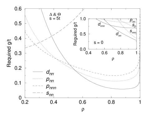
FIG. 2.: Required coupling $g_{\rm BCS}$ to reach a critical temperature $T_{c}=100\mbox{K}(t/1\mbox{eV})$ as a function of the filling $\rho$ for fixed magnitude of the AF background, $s=5t$. The different curves correspond to different shapes of the gap, for the mixed channels, ${\it\Delta}\&{\it\Theta}$. The purely translation invariant and staggered solutions require a much stronger coupling. The inset shows the corresponding result for $s=0$ (no AF).

FIG. 3.: Critical temperature $T_{c}$ as a function of magnitude of antiferromagnetic background $s$ and filling $\rho$, for dominating SC channel ${\it\Delta}\&{\it\Theta}$ and different shapes of the gap. Used parameters here are: $t=0.5\,$eV and $g_{\rm BCS}=0.05\,$eV. (a) $\rho=0.9$ fixed (b) $s=1\,$eV fixed. Labeling of results for different shapes of the gap as in Fig. 1.

FIG. 4.: Magnitude of the superconducting gaps, $|{\it\Delta}|$ and $|{\it\Theta}|$, as a function of temperature $T$ for dominating channels ${\it\Delta}\&{\it\Theta}$. Two neighboring curves show the translation invariant (${\it\Delta}$) and staggered (${\it\Theta}$) parts of the gap. In all cases, $|{\it\Delta}|$ is bigger than $|{\it\Theta}|$. Note that $|{\it\Delta}|$ and $|{\it\Theta}|$ are nearly the same here, which shows that the SC gap closely follows the antiferromagnetic background, as discussed in the text (they become identical for $s\to\infty$). The parameters are $\rho=0.9$, $s=1\,$eV, $t=0.5\,$eV and $g=0.05\,$eV.

FIG. 5.: (a) Superconducting density of states for three different temperatures $T=75\,$K, $65\,$K and $1\,$K. The parameters are the same as in Fig. 4, with a $T_{c}\approx 75\,$K. The chemical potential is at $\omega=0$. (b) Tunneling conductance $dI/dV$ for a superconductor – normal-metal junction as a function of the applied voltage for a sequence of temperatures $T=75,65,55\ldots,5\,$K and $1\,$K. Note that most of the fine structures in the density of states is washed out by temperature effects.

REFERENCES

- [1] For a recent review see: E. Dagotto, Rev. Mod. Phys. 66, 763 (1994).
- [2] See e.g. M. Inui and P.B. Littlewood, Phys. Rev. B 44, 4415 (1991); J.A. Vergés et al., Phys. Rev. B 43, 6099 (1991).
- [3] See e.g. S-W. Cheong et al., Phys. Rev. Lett. 67, 1791 (1991); J.M. Tranquada et al., Phys. Rev. Lett. 64, 800 (1990); G. Shirane et al., Phys. Rev. Lett. 63, 330 (1989).
- [4] Y. Zha, V. Barykin, and D. Pines, Phys. Rev. B 54, 7561 (1996).
- [5] For review see e.g. Chapter 10 in: A.C. Hewson, The Kondo Problem to Heavy Fermions, Cambridge Studies in Magnetism (Cambridge University Press, 1993).
- [6] T.E. Grigereit et al., Phys. Rev. Lett. 73, 2756 (1994).
- [7] for review see e.g. M.B. Maple, Physica B 215, 110 (1995) and references therein.
- [8] P. Monthoux, A.V. Balatsky and D. Pines, Phys. Rev. Lett. 24, 3448 (1991); P. Monthoux and D. Pines, Phys. Rev. B 49, 4261 (1994); K. Ueda, T. Moriya, and Y. Takahashi, J. Phys. Chem. Solids 53, 1515 (1992); N.E. Bickers, D.J. Scalapino, and S.R. White, Phys. Rev. Lett. 62, 961 (1989); A.J. Millis, Phys. Rev. B 45, 13047 (1992).
- [9] J.R. Schrieffer, X.G. Wen, and S.C. Zhang, Phys. Rev. B 39, 11663 (1989); G. Vignale and K.S. Singwi, Phys. Rev. B 39, 2956 (1989); Z.Y. Weng, T.K. Lee, and S.C. Ting, Phys. Rev. B 38, 6561 (1988).
- [10] E. Dagotto, A. Nazarenko, and A. Moreo, Phys. Rev. Lett. 74, 310 (1995); E. Dagotto, A. Nazarenko, A. Moreo, S. Haas, Jour. of superconductivity 9, 379 (1996); A. Nazarenko and E. Dagotto, Phys. Rev. B 53, R2987 (1996).
- [11] For review see e.g. D.J. Scalapino, Phys. Rep. 250, 329 (1995); J.R. Schrieffer, Sol. Stat. Comm. 92, 129 (1994).
- [12] M. Kato and K. Machida, Phys. Rev. B 37, 1510 (1988).
- [13] K. Machida in: A. Narlikar (editor), Studies of high temperature superconductors Vol. 1, Nova Science Publishers (New York, 1989), pp 11.
- [14] For a recent review see R.S. Markiewicz, J. Phys. Chem. Sol. 58, 1179 (1997).
- [15] N. Bulut, cond-mat/9606204, especially Fig. 7; see also D. Duffy, et al., Phys. Rev. B B 56, 5597 (1997).
- [16] R. Heid et al., Phys. Rev. Lett. 74, 2571 (1995).
- [17] See e.g. H.J. Schulz, Phys. Rev. Lett. 65, 2462 (1990). Our notation here follows E. Langmann and M. Wallin, Europhys. Lett. 37, 219 (1997); Phys. Rev. B 55, 9438 (1997).
- [18] See e.g. J.W. Negele and H. Orland, Quantum many-particle systems, Frontiers in Physics, Addison-Wesley (1988). Note that our conventions for the Green functions are such that ( imaginary-time ordering) and differ from the ones used in this book by a sign.
- [19] H. Kleinert, Fortschr. der Physik 26, 565 (1978).
- [20] We write such functions in terms of two translational invariant ones, . The advantage of this is that we then can use the usual Fourier analysis on the entire Brillouin zone and keep track of translational symmetry breaking by the additional index .
- [21] T. Hasegawa, H. Ikuta, and K. Kitazawa in: D.M. Ginsberg (editor), Physical properties of high temperature superconductors, World Scientific Vol. III (1992), p. 526.
- [22] see e.g. V.J. Emery and S.A. Kivelson, Nature 374 434 (1995).