The effect of monomer evaporation on a simple model of submonolayer growth

Abstract

We present a model for thin film growth by particle deposition that takes into account the possible evaporation of the particles deposited on the surface. Our model focuses on the formation of two-dimensional structures. We find that the presence of evaporation can dramatically affect the growth kinetics of the film, and can give rise to regimes characterized by different “growth” exponents and island size distributions. Our results are obtained by extensive computer simulations as well as through a simple scaling approach and the analysis of rate equations describing the system. We carefully discuss the relationship of our model with previous studies of the same physical situation, and we show that our analysis is more general.

The growth of nanostructures and thin films prepared by atomic deposition is recognized to be both a standard and a promising way to prepare new materials [1, 2, 3, 4]. Several models [5, 6, 7, 8, 9] have led to a good understanding of the growth properties in the simplest cases, when only a limited number of physical ingredients are included in the simulations: Deposition, Diffusion and Aggregation as in the DDA model [8]. A drawback of this conceptual simplicity is that the range of experimental situations accurately described by these models is limited. It is actually limited to (beautifully) artificial experimental setups where great care is taken to avoid complications (contamination, surface defects, etc. see for example [10, 11, 12]). Clearly, many (technologically) interesting experimental situations are much more complex. Progress towards their understanding demands the inclusion of processes that have been left out of the first models. For example, including reversible aggregation [13] allows to understand the saturation of island density before island-island coalescence and produces compact islands. In this paper we show the effects of including evaporation of the atoms from the surface.

Evaporation, i.e. the possibility of desorption of adatoms from the surface, is a feature that should be observed for any system at high enough temperatures. In this sense, it is a phenomenon that is as general as the rest of the ingredients of recent models of film growth, and is capable of completely changing the quantitative behaviour of the system (scaling dependence of island density on the deposition parameters, island size distributions …). Moreover, the effects of evaporation have already been studied experimentally [14, 15, 16]. Thin film growth models which include evaporation have already been studied using a mathematical analysis of rate equations [3, 15, 17, 18, 19]. Computer simulations of such models, aiming a quantitative analysis of scaling relations or island size distributions have, to our knowledge, never been carried out. The point is that computer simulations represent an ”exact” way of reproducing the growth, in the sense that they avoid the mean-field approximations of mathematical rate-equations approaches [9, 20, 21]. We find that a careful consideration of the downward transport of monomers from islands leads to results that significantly differ from previous studies [15, 17, 18, 19].

Evaporation is of course not the only process that needs to be added in order to better describe most of the film growth experiments. Other candidates include interlayer transport, particle dissociation (if the incident particles are molecules or clusters rather than atoms) or intricate chemical interactions between adatoms and the surface (for a taste of the real growth world, see for example refs. [22, 23]). These effects are less pervasive than evaporation, but nevertheless, should eventually be considered, keyed to specific experimental systems.

The paper is organized as follows. Section I briefly presents the model and discusses some of its approximations. Then, in section II, we give a rapid overview of the growth of the films when evaporation is taken into account, and try to give a physical intuition for what is going on. After this, section III presents a simple scaling approach which gives the behaviour of the saturation island density as a function of the parameters. This scaling approach is completed in section IV by a more rigorous approach based on a careful analysis of the rate equations of the system. Section V confirms the preceding results by extensive computer simulations of the model. Finally, in section VI, we discuss our results and the differences with the previous approaches [15, 17, 18, 19].

I Presentation of the model

In this work we will describe the properties of a still oversimplified submonolayer thin film growth model which includes the four most important physical ingredients of these systems:

(1) Deposition. We will assume that atoms are deposited at randomly-chosen positions of the surface at a flux $F$ per unit surface per unit time.

(2) Diffusion. Isolated adatoms can move in a random direction by one diameter, or one lattice spacing, which we will take as our unit length. We denote by $\tau$ the characteristic time between diffusion steps.

(3) Evaporation. Isolated adatoms can evaporate off the surface at a constant rate. We denote by $\tau_{e}$ the mean lifetime of a free adatom on the surface. As an approximation, we will assume that the these desorbed atoms do not return to the surface. It is useful to define $X_{S}=\sqrt{D\tau_{e}}$ the mean diffusion length on the substrate before desorption.

(4) Aggregation. If two adatoms come to occupy neighboring sites, they stick to form an island. We will mainly consider the case of irreversible aggregation, but a more general analysis of reversible aggregation, assuming for simplicity the existence of a critical size $i*$ below which islands tend to dissociate is given. In any case, islands are assumed to be immobile and do not evaporate.

In the following, we call particles or adatoms the isolated atoms (or monomers) that are deposited on the surface, and islands a set of connected particles (thus excluding the monomers).

Some remarks on the assumptions of this simple model regarding its connection to the experiments are now addressed.

(a) Second layer— When a particle “falls” on top of an island, we assume that the particle deposited on the second layer moves and evaporates essentially as any other particle, except that its diffusion constant and evaporation rate now correspond to the process ocurring on a substrate of the same element as the deposited particles. Practically, the mean diffusion length on the island before desorption, defined as $X_{S}^{*}=\sqrt{D^{*}\tau_{e}^{*}}$, where the ^∗ indicate the values on the island, can be different from $X_{S}$. As the simplest scenario, we assume that when the particle reaches the border of the island, it immediately jumps down and increases the area of the island. We discuss when this effect can be ignored without affecting the scaling results, which leads to applications to situations in which downward transport of monomers from islands is highly improbable. This could be the case when: (i) there is a barrier [24] at the edges of the (first layer) clusters which prevents single particles from “falling” on the substrate and/or (ii) Particle diffusion on the second layer is much smaller than diffusion on the substrate.

(b) Island diffusion—We neglect in this model the possibility for dimers, trimers or larger islands to diffuse on the substrate. Island diffusion has been observed in experiments [27] and molecular-dynamics simulations [28]. The effects of island diffusion on the growth of thin films without evaporation have been addressed in Refs. [8, 20, 21, 5, 29, 30]. While these effects are significant since they change the growth exponents, they do not modify fundamentally the growth mechanisms. We assume that the same is true when evaporation is included.

We study here the first stages of the growth, roughly until the number of islands on the substrate saturates. The reason is that it is in this stage that such a simplified model can be of some help to experimentalists who want to understand the microscopic processes present in their experiments. These fundamental microscopic processes are most easily detected in the first stages of the growth, since in the subsequent stages additional processes can be involved (additional diffusion paths, interlayer transport, geometrical details of the lattice…).

II Qualitative description

Before going into the details of the calculations and their confirmation by computer simulations, we present a simple picture of the growth mechanisms of the submonolayer structures under consideration. For simplicity, we only consider here the case $i^{*}=1$, i.e. irreversible aggregation and we neglect the particles deposited on top of the islands (despite the apparent lack of generality of this last hypothesis, the results obtained here are quite general, as we show in section IV).

The qualitative evolution of the system is essentially as follows. The system initiates as a clean empty surface. Monomers are then deposited at a constant rate on the surface and are allowed to diffuse and/or desorb (evaporate). When two (or more) monomers meet, they aggregate irreversibly to form a static island. As more of these encounters occur, the island density increases with time and islands become larger by capturing adatoms. At some point, islands are so large that they start touching (coalescing), and monomers are rapidly captured. These two effects lead to a saturation in the number of islands. Interestingly, the saturation is attained when the surface coverage reaches a value close to .15, independently of the parameter values. This last point is discussed in detail below. We now turn to a more detailed discussion of the evolution of the systems in two limiting cases : complete condensation (evaporation is negligible) and strong evaporation.

First consider the situation where evaporation is negligible. This means that atoms deposited on the surface almost never evaporate before aggregating (after this, they are safe since islands do not evaporate). This situation can be expected to happen when $X_{S}\gg\ell$ where $X_{S}=\sqrt{D\tau_{e}}$ is the adatom diffusion length on the substrate before desorption and $\ell$ is the typical distance between islands. Fig  1a shows the evolution of the monomer and island densities as a function of deposition time. We see that the monomer density rapidly grows, leading to a rapid increase of island density by monomer-monomer encounter on the surface. This goes on until the islands occupy a significant fraction of the surface, roughly 1%. Then, islands capture rapidly the monomers, whose density decreases. As a consequence, it becomes less probable to create more islands, and we see that their number increases more slowly. When the coverage reaches a value close to 15%, coalescence will start to decrease the number of islands. The maximum number of islands $N_{max}$ is thus reached for coverages around 15%. Concerning the dependence of $N_{max}$ as a function of the model parameters, the DDA and related models have shown that the maximum number of islands per unit area formed on the surface scales as $N_{max}\simeq(F/D)^{1/3}$, or $\ell_{CC}\simeq(F/D)^{-1/6}$ [5, 18, 19] where $CC$ stands for Complete Condensation. These values are independent of $\tau_{e}$ since evaporation is not significant.

(a)      (b)

FIG. 1.: Evolution of the monomer and island densities as a function of the deposition time (in monolayers) for different limits : (a) complete condensation, $F=10^{-8},\ \tau_{e}=10^{10}\ (\tau=1)$. These values mean : $X_{S}=10^{5}$ and $\ell_{CC}=22$ (b) important evaporation, $F=10^{-8},\ \tau_{e}=600\ (\tau=1)$. These values mean : $X_{S}=25$ and $\ell_{CC}=22$. In (b) the ”sticking” curve represents the total number of particles actually present on the surface (the coverage) divided by the total number of particles sent on the surface (F t). It would be 1 for the complete condensation case, neglecting the monomers that are deposited on top of the islands. The island density curve has been shifted vertically by (+1). The solid line represents the constant value expected for the monomer concentration, while the dashed line corresponds to the linear increase of the island density (see text).

When $\tau_{e}$ decreases (i.e. as the evaporation rate increases), $X_{S}$ decreases and eventually becomes smaller than $\ell_{CC}$. In this regime, evaporation is going to significantly alter the growth dynamics, as shown in Fig  1b. The main point is that now the monomer density becomes roughly a constant, since it is now mainly determined by the balancing of deposition and evaporation. As expected, the constant concentration equals $F\tau_{e}$, as shown by the solid line. Then the number of islands increases linearly with time (the island creation rate is roughly proportional to the square monomer concentration). We also notice that only a small fraction (1/100) of the monomers do effectively remain on the substrate, as shown by the low sticking coefficient value at early times (the sticking coefficient is the ratio of particles on the substrate (the coverage) over the the total number of particles sent on the surface (Ft)). This can be understood by noting that the islands grow by capturing only the monomers that are deposited within their ”capture zone” (comprised between two circles of radius $R$ and $R+X_{S}$ if we neglect $X_{S}^{*}$, see Figure  2). The other monomers evaporate before reaching the islands. As in the case of complete condensation, when the islands occupy a significant fraction of the surface, they capture rapidly the monomers. This has two effects : the monomer density starts to decrease, and the sticking coefficient starts to increase. Shortly after, the island density saturates and starts to decrease because of island-island coalescence.

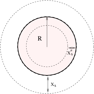
FIG. 2.: Schematic capture zone for an island in presence of atom evaporation. $X_{S}^{*}$ stands for the mean length before desorption for an atom diffusing on top of an island, whereas $X_{S}$ corresponds to the same parameter on the substrate (see text). The sizes of the capture zones will be justified below, in section IV.

If $\tau_{e}$ is further decreased (precisely $\tau_{e}\leq\tau$ i.e. the time a particle remains on the surface is less than the time it needs to move), then, clearly, diffusion plays no role (”$X_{S}\leq 1$”). In this situation, islands are formed by direct impingement of incident atoms as first neighbors of adatoms, and grow by direct impingement of adatoms on the island boundary. This situation, although apparently uncommon, is not physically impossible and it also allows us to test our predictions over a larger range of parameters.

III Scaling arguments

In this section we present simple scaling arguments that allow to find the dependence of the maximum island density $N_{max}$ as a function of the deposition parameters (Flux F, Diffusion time $\tau$ and Evaporation time $\tau_{e}$). These arguments were originally formulated in [5] for the special case of deposition without evaporation on a high-symmetry terrace. Here, the argument is extended to the case of non-negligible evaporation. We recall that the atomic size is taken as the length unit. For simplicity, we neglect in this section the effects of deposition on the second layer : they will be studied in great detail in the next section. We will show there that the regime studied in this section corresponds to a large range of physical situations.

The first stage of the argument requires the determination of the nucleation rate per unit surface and time, $1/\tau_{\rm nuc}$. A nucleation event takes place when two adatoms meet. This happens with a probability per unit time $D\rho^{2}$, where $D=1/(4\tau)$ is the adatom diffusion constant, and $\rho$ the adatom density. Thus,

$$\frac{1}{\tau_{\rm nuc}}\approx D\rho^{2}$$ (1)

Another, independent equation can be written down to relate the nucleation rate and the island density $N$. It states that in the area $\ell_{s}^{2}=1/N$ occupied by an island, only one (on average) nucleation event takes place, during the time $t_{c}$ needed for the growing islands to come into contact. Thus,

$$\frac{1}{\tau_{\rm nuc}}\approx\frac{N}{t_{c}}\;.$$ (2)

The time $t_{c}$ is readily computed by knowing the growth velocity of an island, which in turn requires the knowledge of the adatom density. We consider in the following the situations of interest for this paper.

A No evaporation, compact 2-D islands

The adatom density results in this case from a balance between deposition at a rate $F$ and capture by the stable islands at a rate $D\rho N$, so that

$$\rho\approx F/(DN)\approx F\ell_{s}^{2}/D\$$ (3)

The area of an island of linear size $R$ increases by capture of all adatoms falling in an area $\ell_{s}^{2}$, so that $R^{2}\approx F\ell_{s}^{2}t$. At $t=t_{c}$, $R\approx\ell_{s}$, and thus $t_{c}\approx 1/F$. Using (1) and (2) one finds $D\rho^{2}\approx FN$. From (3), $N\approx F\ell_{s}^{4}/D$, or [5, 18, 19]

$$N\approx\left(\frac{F}{D}\right)^{1/3}\;.$$ (4)

The value $1/3$ corresponds to the special case $i^{*}=1$ of the general formula $i^{*}/(2+i^{*})$ for the exponent [5, 18, 19].

B Strong evaporation

Strong evaporation means the adatoms are more likely to disappear due to desorption, with probability $1/\tau_{e}$ per unit time and site, than to be captured by an island. Therefore, the adatom diffusion length before desorption, $X_{S}=\sqrt{D\tau_{e}}$, is shorter than the average island-island distance, $\ell_{s}$. In this case, the adatom density results from a balance between deposition and desorption at a rate $\rho/\tau_{e}$, so that

$$\rho\approx F\tau_{e}\approx FX_{S}^{2}/D.$$ (5)

A growing island is only able to capture the adatoms falling at a distance smaller than the adatom diffusion length before desorption, $X_{S}$ (see Figure  2). If $X_{S}$ is smaller than the island size $R$, the island will capture the adatoms falling inside an annulus of width $\approx X_{S}$ around its border, as well as those directly impinging on its edge. Since the area of the annulus is $\approx RX_{S}$ if $R\gg X_{S}$, at time $t$ one has $R\approx F(1+X_{S})t$. At $t=t_{c}$, $R\approx\ell_{s}$, and thus $t_{c}\approx\ell_{s}/[F(1+X_{S})]\approx 1/[FN^{1/2}(1+X_{S})]$. Direct impingement is also important for nucleation, so that (1) becomes

$$(F+D\rho)\rho\approx F(1+X_{S}^{2})\rho\approx F^{2}\tau_{e}(1+X_{S})^{2}\$$ (6)

where we also used (5).

From (2) and (6), one finds $F^{2}\tau_{e}(1+X_{S})^{2}\approx F(1+X_{S})N^{3/2}$, or

$$N\approx\left(F\tau_{e}\right)^{2/3}\left(1+X_{S}\right)^{2/3}\;.$$ (7)

For a comparison with previous results, it may be worth it to rederive (7) for any value of $i^{*}$. The nucleation rate reads, for any $i^{*}$, $(F+D\rho)N_{i^{*}}$, where $N_{i^{*}}$ is the density of critical nuclei (clusters of size $i^{*}$). Following Refs. [18, 19], we assume that $N_{i^{*}}$ satisfies Walton’s relation $N_{i^{*}}\sim\rho^{i^{*}}$. Inserting into (6) yields $1/\tau_{\rm nuc}\approx F(F\tau_{e})^{i^{*}}(1+X_{S})^{2}$. Finally, using (2) yields $F(F\tau_{e})^{i^{*}}(1+X_{S})^{2}\approx F(1+X_{S})N^{3/2}$, or

$$N\approx\left(F\tau_{e}\right)^{2i^{*}/3}\left(1+X_{S}\right)^{2/3}\;.$$ (8)

Note that the validity of Walton’s relation in the presence of strong desorption is highly hypothetical. It is a point which we reserve for future work. In the rest of the paper, we only consider the case $i^{*}=1$. In section IV, the results for $i^{*}=1$ are derived by a more rigorous rate-equations [31] approach.

C Crossover scaling

We will derive here an approximate analytic expression for the crossover scaling function connecting the complete condensation, diffusion and direct impingement regimes described previously. In other words, we will compute the maximum island density $N_{max}$ as a function of $F$, $\tau$ and $\tau_{e}$. We will then show that, if we measure all lengths in terms of $X_{S}$, $N_{max}(F,\tau,\tau_{e})$ is a function of its arguments only through a special combination: $X_{S}^{2}N_{max}=g_{evap}(X_{S}^{2}N_{evap})$, where $N_{evap}=\left[(1+X_{S})F\tau_{e}\right]^{2/3}$, and $g_{evap}(x)$ satisfies

$$g_{evap}(x)\sim\cases{{x^{1/2}}&{\rm for} ~{}$x\to\infty$,\cr\cr{{x}}&{\rm for}~{} $x\to 0$.\cr}$$ (9)

To do this, we assume that the islands are large enough with respect to the atomic size, that we can neglect the curvature of their boundary. Then, the adatom density in the region between two islands whose edges are at a distance $\ell$, obeys the equation

$$\dot{\rho}=F+D\nabla^{2}\rho-\frac{\rho}{\tau_{e}}\;,$$ (10)

with the boundary conditions $\rho(\pm\ell/2)=0$ (the origin being midway between the islands).

In the quasi-stationary approximation, $\dot{\rho}\approx 0$, and equation (10) can be solved. The solution reads

$$\rho(x)=F\tau\left[1-\frac{\cosh(\kappa x)}{\cosh(\kappa\ell/2)}\right]\;,$$ (11)

where $\kappa=1/X_{S}$

This formula is needed to compute the nucleation rate $D\rho^{2}$. The latter is a mean field quantity, independent of $x$. Letting thus $x=0$ in (11)–since the highest nucleation probability is at the terrace centre, given the symmetry of our problem–one finds

$$\rho=F\tau\left[1-\frac{1}{\cosh(\kappa\ell/2)}\right]=2F\tau\frac{\sinh^{2}(\kappa\ell/4)}{\cosh(\kappa\ell/2)}\;,$$ (12)

where we used the identity $\cosh(x)-1=2\sinh^{2}(x/2)$.

The next task is the determination of the total island density $N$. Its time variation is simple: $N$ increases each time a new island is nucleated, so that $(\dot{N})_{1}=D\rho^{2}$. On the other hand, $N$ decreases when two islands touch and coalesce. Following previous authors [17, 19], we write $(\dot{N})_{2}=-(d{\cal A}/dt)N^{2}$, where ${\cal A}\approx R^{2}$ is the average area of an island of linear size $R$. This means that coalescence results from binary encounters of immobile islands, whose area increases at a rate $d{\cal A}/dt$. Collecting $(\dot{N})_{1}$ and $(\dot{N})_{2}$ yields

$$\dot{N}=D\rho^{2}-\frac{d{\cal A}}{dt}N^{2}\;.$$ (13)

By definition, $N_{max}$, which is what we are interested in, satisfies $\dot{N}=0$. This means that the maximum of the island density can be found by balancing the nucleation rate against the coalescence rate, and that the balance is reached when the island size $R\approx\ell$. One can thus write

$$D\rho^{2}\approx\left(\frac{d{\cal A}}{dt}\right)_{R\approx\ell}N_{max}^{2}\;.$$ (14)

The growth rate of an island can be computed assuming that its radius is large with respect to the atomic size. One can then treat the island edges as straight steps, which yields

$$\frac{dR}{dt}\approx FX_{S}\tanh(\kappa\ell/2)\;.$$ (15)

Since $d{\cal A}/dt\approx RdR/dt$, one finds

$$\frac{d{\cal A}}{dt}|_{R=\ell}\approx FX_{S}\ell\tanh(\kappa\ell/2)\;.$$ (16)

Note that the two limits $({d{\cal A}}/{dt})|_{R=\ell}\approx F\ell^{2}$ and $({d{\cal A}}/{dt})|_{R=\ell}\approx F\ell X_{S}$ are well reproduced for $\kappa\ell\ll 1$ and for $\kappa\ell\gg 1$, respectively. In fact, in the limit $X_{S}\to 0$, the area increase is $FR$, due to direct impingement. In order to interpolate all the way through to this regime, we finally write

$$\frac{d{\cal A}}{dt}|_{R=\ell}\approx F(1+X_{S})\ell\tanh(\kappa\ell/2)\;.$$ (17)

In the limit where the diffusion length $X_{S}$ becomes very small, the nucleation probability is also determined by direct impingement of a beam atom on a nucleus, which is described by $F\rho$. Then, the nucleation term in (14) reads

$$(F+D\rho)\rho\approx F\left[1+X_{S}^{2}\frac{\sinh^{2}(\kappa\ell/4)}{\cosh(\kappa\ell/2)}\right]\left[F\tau_{e}\frac{\sinh^{2}(\kappa\ell/4)}{\cosh(\kappa\ell/2)}\right]\;.$$ (18)

In fact, a simpler approximate expression will be used, which reproduces the correct limiting behaviour at large and small $X_{S}$:

$$(F+D\rho)\rho\approx\frac{\left(1+X_{S}\right)^{2}}{\tau_{e}}\left[F\tau_{e}\frac{\sinh^{2}(\kappa\ell/4)}{\cosh(\kappa\ell/2)}\right]^{2}\;.$$ (19)

Finally, (17) and (19) yield

$$\frac{\left(1+X_{S}\right)^{2}}{\tau_{e}}\left[F\tau_{e}\frac{\sinh^{2}(\kappa\ell/4)}{\cosh(\kappa\ell/2)}\right]^{2}\approx F(1+X_{S})\ell\tanh(\kappa\ell/2)N_{max}^{2}\;,$$ (20)

or, letting $\ell=N_{max}^{-1/2}$,

$${\left(1+X_{S}\right)}(F\tau_{e})\approx\left[\frac{\cosh(\kappa N_{max}^{-1/2}/2)}{\sinh^{2}(\kappa N_{max}^{-1/2}/4)}\right]^{2}\tanh(\kappa N_{max}^{-1/2}/2)N_{max}^{3/2}\;.$$ (21)

This is the announced crossover scaling formula, in implicit form. It can be cast in the form:

$${(1+X_{S})}X_{S}^{3}(F\tau_{e})\approx\left[\frac{\cosh(\kappa N_{max}^{-1/2}/2)}{\sinh^{2}(\kappa N_{max}^{-1/2}/4)}\right]^{2}\tanh(\kappa N_{max}^{-1/2}/2)(X_{S}^{2}N_{max})^{3/2}\;,$$ (22)

or,

$${\left(1+X_{S}\right)}X_{S}^{5}\left(\frac{F}{D}\right)=f_{evap}(X_{S}N_{max}^{1/2})\;,$$ (23)

where

$$f_{evap}(x)=\left[\frac{\cosh\left(\frac{1}{2x}\right)}{\sinh^{2}\left(\frac{1}{4x}\right)}\right]^{2}\tanh\left(\frac{1}{2x}\right)x^{3}\;.$$ (24)

Letting $N_{evap}=[(1+X_{S})F\tau_{e}]^{2/3}$, and inverting $f$, one finds as promised:

$$X_{S}^{2}N_{max}=g_{evap}(X_{S}^{2}N_{evap})\;.$$ (25)

IV Rate equations

In this section we will study the model taking into account the particles deposited on top of the islands with their specific diffusion and evaporation parameters. We will show that for a large range of parameters, the exponents are the same as those predicted by the preceding analysis. We use a ”rate-equations” approach which has been shown to give a good description of the submonolayer regime [6, 9, 17, 19, 31]. For the sake of completeness, we include a detailed calculation of the “cross sections” for monomer capture. These “cross sections” have also been calculated in [9, 15, 17] for example.

We will not keep careful track of many of the numerical geometric constants. The rate equation describing the time evolution of the density $\rho$ of monomers on the surface will be, to lowest relevant orders in F:

$${d\rho\over dt}=F(1-\theta)-{\rho\over\tau_{e}}-F\rho-2\sigma_{o}\rho-\sigma_{i}N$$ (26)

The first term on the right hand size denotes the flux of monomers onto the island free surface, ($\theta$ is the island coverage discussed below). The second term represents the effect of evaporation, i.e. monomers evaporate after an average time $\tau_{e}$. The third term is due to the possibility of losing monomers by effect of direct impingement of a deposited monomers right beside a monomer still on the surface to form an island. As discussed above, this “direct impingement” term is usually negligible, and indeed will turn out to be very small in this particular equation, but the effect of direct impingement plays a crucial role in the kinetics of the system in the high evaporation regimes. The last two terms represent the loss of monomers by aggregation with other monomers and with islands respectively. The factors $\sigma_{o}$ and $\sigma_{i}$ are the “cross sections” for encounters and will be calculated below.

The number $N$ of islands will be given by:

$${dN\over dt}=F\rho+\sigma_{o}\rho$$ (27)

where the first term represents the formation of islands due to direct impingement of deposited monomers next to monomers already on the surface, and the second term accounts for the formation of islands by the encounter of monomers diffusing on the surface.

For the island coverage $\theta$ i.e. the area covered by all the islands per unit area, we have:

$${d\theta\over dt}=2\left[F\rho+\sigma_{o}\rho\right]+\sigma_{i}N+JN$$ (28)

The term in brackets represents the increase of coverage due to formation of islands of size 2 (i.e. formed by two monomers) either by direct impingement or by monomer-monomer aggregation. The next term gives the increase of coverage due to the growth of the islands as a result of monomers aggregating onto them by diffusion, and the last term represents the growth of the islands due to direct impingement of deposited monomers onto their boundary, or directly on the island. The estimation of the value of J is carried out below. The total surface coverage is given by $\theta+\rho\sim\theta$ except at very short times.

The next step in the analysis consists in estimating the cross sections $\sigma_{o}$ and $\sigma_{i}$. This is done by evaluating the diffusive flux of monomers into a single single solitary island represented by an absorbing disk of radius $R$ centered at the origin (throughout this analysis $R$ stands for the typical island radius). The typical radius $R$ of the islands will be taken to be:

$$R\sim\left({\theta\over N}\right)^{1/2}$$ (29)

The cross sections are evaluated in the quasistatic approximation, which consists in assuming that $R$ does not vary in time and that the system is at a steady state. Thus, we have to solve the equation

$$D\left({\partial^{2}P\over\partial r^{2}}+{1\over r}{\partial P\over\partial r}\right)+F-{1\over\tau_{e}}P({\bf r})=0$$ (30)

subject to the boundary condition $P(r=R)=0$, where $P({\bf r})$ is the monomer concentration at position ${\bf r}$ and $D$ is the diffusion constant of the monomers. The solution is given by:

$$P({\bf r})={F\tau_{e}}\left(1-{K_{0}(r/X_{S})\over K_{0}(R/X_{S})}\right),$$ (31)

where $X_{S}=(D\tau_{e})^{1/2}$ can be identified as the characteristic distance traveled by a monomer before evaporation, and $K_{0}(x)$ is the modified Bessel function of order zero. We can rewrite Eq. 31 as:

$$P({\bf r})=\rho\left(1-{K_{0}(r/X_{S})\over K_{0}(R/X_{S})}\right),$$ (32)

where $\rho$ is the monomer density appearing in the rate equations, so that $P({\bf r})\to\rho$ far from the islands. This, again, is a mean field way of including the effects of the other islands in the flux of monomers into the island in consideration. The cross section $\sigma_{i}$ can then be calculated as the total diffusive flux of monomers into the boundary,

$$\sigma_{i}=2\pi RD\left({dP\over dr}\right)_{r=R}=2\pi D\rho\left(R\over{X_{S}}\right){K_{1}(R/X_{S})\over K_{0}(R/X_{S})}$$ (33)

The cross section for monomer-monomer encounters $\sigma_{o}$ is obtained from the same formula substituting $R$ by the monomer radius, and $D$ by $2D$ as corresponds to relative diffusion.

The rate equations, with the explicit expressions for $\sigma_{i}$ and $\sigma_{o}$ are still too complicated to solve exactly. At best we can focus on extreme cases. The first step then is to evaluate the extreme values of $\sigma_{i}$ for the case in which $R\gg X_{S}$ and $R\ll X_{S}$. Using the known asymptotic values of the Bessel functions, and once again omitting numerical constants, we have

$$\sigma_{i}\sim\cases{{D\rho R\over{X_{S}}}&for $R\gg X_{S}$,\cr\cr{D\rho\over\ln(X_{S}/R)}&for $R\ll X_{S}$.\cr}$$ (34)

From here on we will neglect the logarithmic variations appearing in the cross section. To evaluate $\sigma_{o}$ we notice that the monomer radius is a small constant (it is usually taken as half the unit of length), so for all values of $X_{S}$, to a good approximation we have

$$\sigma_{o}\sim D\rho$$ (35)

Formally, the diffusive cross section for monomers should vary in the case $X_{S}\ll 1$, but this is of no consequence since in that regime the contributions from diffusion are negligible.

Now we turn to the evaluation of the direct impingement flux $J$. As was the case above, the exact evaluation of $J$ is rather difficult, as it results from the solution of a moving boundary problem. Thus, once again, we must resort to a quasistatic approximation.

The flux $J$ will consist of two terms, $J_{b}$ the contribution due to direct impingement at the exterior boundary of the island, i.e. on the substrate, and $J_{i}$ the contribution due to particles falling on the island, diffusing to the boundary, and “falling” over the edge to increase the size of the island. We will continue to assume that the islands are compact, thus, the contribution due to direct impingement at the boundary will be given by $FR$ (where we have omitted geometrical constants). To evaluate the second contribution we must solve:

$$D^{*}\left({\partial^{2}P\over\partial r^{2}}+{1\over r}{\partial P\over\partial r}\right)+F-{1\over\tau_{e}^{*}}P({\bf r})=0$$ (36)

subject to the boundary condition $P(r=R)=0$. We recall that $D^{*}$ and $\tau_{e}^{*}$ represent the values of the diffusion constant and evaporation time of the particles on a substrate of their same species (clearly, for homoepitaxy $D^{*}=D$ and $\tau_{e}^{*}=\tau_{e}$). The boundary condition corresponds to the simplest situation, in which there is no barrier at the edge of the island and every particle reaching the boundary falls. The increase in coverage will be given by the total flux accross the barrier, i.e. $J_{i}\sim-RD^{*}{\partial P\over\partial r}$. In writing this equation we have assumed that no nucleation occurs on top of the island, for this to be the case, we must require that $P_{max}\ll 1$ on the island, which will be the case for small enough $F$.

The solution to the above equation can be readily found, and from it we find that

$$J_{i}\sim RX_{s}^{*}F\left({I_{1}(R/X_{s}^{*})\over I_{0}(R/X_{s}^{*})}\right)$$ (37)

where $X_{s}^{*}=\sqrt{D^{*}\tau_{e}^{*}}$ is the typical distance a monomer can diffuse on an island before desorption, and $I_{0}(x)$ and $I_{1}(x)$ are modified Bessel functions. Again using the known properties of Bessel functions, we can distinguish two limiting behaviors:

$$J_{i}\sim\cases{{FR^{2}}&for ~{}$R\ll X_{S}^{*}$,\cr{{FRX_{S}^{*}}}&for` $R\gg X_{S}^{*}$.\cr}$$ (38)

A High Evaporation Regimes

We are now in a position to analyse the limiting cases of the system described by the rate equations. First we consider the new behaviour brought about by the presence of evaporation. We define the high evaporation regimes as the systems in which all but the first two terms on the right-hand side of Eq. 26 are negligible. Then, since the coverage is small, we have

$${d\rho\over dt}\sim F-{\rho\over\tau_{e}},$$ (39)

and $\rho$ reaches a steady state value $\rho=F\tau_{e}$ in a time of order $\tau_{e}$. Thus, as mentioned above, the high evaporation regimes are characterized by having a constant monomer density (after an initial transient) throughout most of the evolution of the system. Under these circumstances Eq. 27 becomes trivial and predicts that the number of islands at time $t$ is given by

$$N\sim F^{2}\tau_{e}\left[1+X_{S}^{2}\right]t$$ (40)

If the evaporation rate is very high, so that $X_{S}\ll 1$, then even the smallest islands at the earliest stages of evolution will satisfy the relation $R\gg X_{S}$ (will refer to this situation as extreme incomplete condensation). If we assume that the diffusion length on the islands $X_{s}^{*}$ is also much less than one, then Eq. 28 becomes

$${d\theta\over dt}\sim FRN\sim F(\theta N)^{1/2},$$ (41)

where we have neglected the increase of coverage due to the formation of small new islands in Eq. 28, as most of the coverage is due to the large islands. And the number of islands evolves as

$$N\sim F^{2}\tau_{e}t,$$ (42)

Solving for $\theta$, we obtain

$$\theta\sim F^{4}\tau_{e}t^{3}.$$ (43)

Now comes a crucial assumption, namely that coalescence occurs when the coverage reaches a fixed constant value, say $\theta_{c}=1/6$, and that this value is essentially independent of the details of how the surface is covered. Thus, the time $t_{c}$ at which coalescence occurs will be

$$t_{c}\sim\left(F^{4}\tau_{e}\right)^{-1/3}$$ (44)

Since the number of islands is a monotonically increasing function of time up to the time of coalescence, we can estimate the maximum number of islands on the surface as

$$N_{max}\sim N(t_{c})\sim\left(F\tau_{e}\right)^{2/3}$$ (45)

If instead we consider the case in which $R\gg X_{s}^{*}\gg 1$, and $X_{s}\ll 1$, then island formation will still only occur via direct impingement, but the increase of coverage will be primarily due to monomers landing in the capture zone on the islands. In this situation, we will have

$${d\theta\over dt}\sim X_{S}^{*}FRN,$$ (46)

and again

$$N\sim F^{2}\tau_{e}t,$$ (47)

from which we obtain

$$\theta\sim F^{4}\tau_{e}X_{s}^{*}t^{3}.$$ (48)

The coalescence time can be estimated as before, leading to a maximum number of islands that scales as

$$N_{max}\sim N(t_{c})\sim\left(F\tau_{e}X_{s}^{*}\right)^{2/3}$$ (49)

If we instead consider the case of extreme mismatch between the materials, so $X_{S}\ll 1$ but $X_{S}^{*}\gg R$ throughout the evolution of the system, the the capture zone on the islands becomes the whole island, at which point the coverage increases as

$${d\theta\over dt}\sim F\theta,$$ (50)

where we used $NR^{2}\sim\theta$. Coalescence then occurs at at a time $t_{c}\sim 1/F$, and the maximum number of islands at that time will be

$$N_{max}\sim F\tau_{e},$$ (51)

Different and more interesting regimes exist for the situation in which $X_{S}\gg 1$, still in the high evaporation regime, i.e. the evolution of the monomer density is still essentially controlled solely by the deposition and evaporation. This requirement actually limits the value of $X_{S}$. The upper bound for the range of $X_{S}$ in which this situation prevails is discussed below. First we consider the case in which eventually $R\gg X_{S}^{*}$ as well. In this situation, the increase in coverage is due mainly to the particles deposited within the capture zone of the islands, which we assume to be relatively large.

For times long enough for these conditions to prevail, the evolution of the coverage will be given by

$${d\theta\over dt}\sim(X_{S}+X_{S}^{*})RFN,$$ (52)

and the number of islands will evolve as

$${dN\over dt}\sim F^{2}\tau_{e}X_{S}^{2}.$$ (53)

Thus, solving for the coverage, we find that

$$\theta\sim F^{4}X_{S}^{2}(X_{S}+X_{S}^{*})^{2}\tau_{e}t^{3}.$$ (54)

Once again we assume that coalescence becomes important at a value of $\theta$ of the order of unity, so that the coalescence time in this regime will be given by

$$t_{c}\sim(F^{4}X_{S}^{2}(X_{S}+X_{S}^{*})^{2}\tau_{e})^{-1/3},$$ (55)

and the maximum number of islands will be given by

$$N_{max}\sim\left({FX_{S}^{2}\tau_{e}\over X_{S}+X_{S}^{*}}\right)^{2/3}.$$ (56)

Note that ignoring the particles that land on the islands, i.e. taking $X_{S}^{*}=0$, as if there was an infinite edge berrier, yields the same scaling as would be expected if $X_{S}\gg X_{S}^{*}$, and also the same scaling as would be expected in homoepitaxy, where $X_{S}=X_{S}^{*}$. Thus, ignoring these ”second layer” particles is not crucial for the calculation of the exponents, at least for a large range of the values of the parameters.

If we now assume that eventually $R\gg X_{S}$, but that $X_{S}^{*}\gg R$, then once again the coverage will evolve as

$${d\theta\over dt}\sim F\theta.$$ (57)

Coalescence then occurs at at a time $t_{c}\sim 1/F$, and the maximum number of islands at that time will now be given by

$$N_{max}\sim F\tau_{e}X_{S}^{2}$$ (58)

This is the result obtained by Venables, as we discuss later (section VI).

B Low evaporation rates

If $\tau_{e}$ is further increased, then the system does not reach the regime characterized in the previous section. As mentioned above, this regime holds as long as $R\gg X_{S}$ beyond certain point in the evolution of the system. We can estimate the value of $\tau_{e}$ at which this condition never holds, i.e. when $X_{S}\sim R_{max}$, where the maximum island size $R_{max}$ can be estimated through

$$R_{max}\sim\left({\theta_{c}\over N_{max}}\right)^{1/2}\sim\tau_{e}^{-1/2}F^{-1/3}D^{-1/6}$$ (59)

Hence, the evaporation time above which the condition $R\gg X_{S}$ never holds is such that

$$X_{S}=\left({D\tau_{e}}\right)^{1/2}\sim R_{max}\sim\tau_{e}^{-1/2}F^{-1/3}D^{-1/6}$$ (60)

that is,

$$\tau_{e}^{(2)}\sim(FD^{2})^{-1/3}={\ell_{CC}}^{2}\tau$$ (61)

For evaporation times above $\tau_{e}^{(2)}$ the monomers are expected to travel distances much longer than the largest typical island sizes. At this point it is important to realize that our criterion for the onset of coalescence, $\theta\sim 1$, is equivalent to the requirement $R\sim\ell$, where $\ell\sim N^{-1/2}$ is the typical distance between islands. Thus, for evaporation times much larger than $\tau_{e}^{(2)}$, a great part of the evolution of the system takes place with the monomers traveling distances which are greater than the inter-island distances. During this phase we expect the effects of evaporation to be negligible. In effect, if $\tau_{e}>\tau_{e}^{(2)}$, the kinetics of the monomer density is no longer determined solely by the evaporation, but rather, it is eventually determined by the aggregation processes.

At very short times the number of islands is expected to be very small. Therefore, in the early stages of evolution, they cannot affect the monomer density. Thus, the early stages of evolution are expected to be similar to those of the previous regime, for example:

$$\rho\sim F\tau_{e},\qquad N\sim F^{2}X_{S}^{2}\tau_{e}t\qquad\theta\sim F^{3}X_{S}^{4}\tau_{e}t^{2}.$$ (62)

This situation is expected to hold until the number of islands is large enough, so that the term $\sigma_{i}N$ is no longer negligible when compared to $F$. That is, until a time $t_{xx}$ such that

$$\sigma_{i}N\sim DF^{3}X_{S}^{2}\tau_{e}^{2}t_{xx}\sim F,$$ (63)

from which we obtain

$$t_{xx}\sim(F^{2}X_{S}^{4}\tau_{e})^{-1}.$$ (64)

As expected, the number of islands at $t_{xx}$ is $N(t_{xx})\sim 1/X_{S}^{2}$, indicating that evaporation effects “turn” off once the typical inter-island distance is smaller than $X_{S}$. For times beyond $t_{xx}$ all evaporation effects become negligible and our rate equations reduce to those given by Tang [6] for a system without evaporation (plus the direct impingement terms that are negligible in this limit) for which the results are well known. Namely the time at which coalescence occurs is given by

$$t_{c}\sim 1/F$$ (65)

and the maximum number of islands nucleated on the surface is

$$N_{max}\sim\left({F\over D}\right)^{1/3}$$ (66)

We can now summarize now the various regimes obtained. There are three principal regimes which are spanned as the evaporation time $\tau_{e}$ decreases. We call them, in this order, the complete condensation regime where evaporation is not important, the diffusion regime where islands grow mainly by diffusive capture of monomers and finally the direct impingement regime where evaporation is so important that islands can grow only by capturing monomers directly from the vapor. Within each of these regimes, there are several subregimes characterized by the value of $X_{S}^{*}$, the desorption length on top of the islands. We use $\ell_{CC}\equiv(F\tau)^{-1/6}$, the typical island-island distance when there is no evaporation and $R_{max}$ as the maximum island radius, reached at the onset of coalescence.

complete  condensation $X_{S}\gg\ell_{CC}$

$$N_{max}\sim F^{1/3}\tau^{1/3}{\rm\ for\ any\ X_{S}^{*}}$$ (67)

diffusive growth $1\ll X_{S}\ll\ell_{CC}$

$$N_{max}\sim\cases{(FX_{S}^{2}\tau_{e})^{2/3}(X_{S}+X_{S}^{*})^{-2/3}&{\rm if}~{}~{}~{}~{} $X_{S}^{*}\ll R_{max}$ \ (a)\cr\cr F\tau_{e}X_{S}^{2}&{\rm if}~{}~{}~{}~{} $X_{S}^{*}\gg R_{max}$ \ (b)\cr\cr}$$ (68)

with $R_{max}\sim(X_{S}+X_{S}^{*})^{1/3}(FX_{S}^{2}\tau_{e})^{-1/3}$, which gives for the crossover between regimes (a) and (b) : $X_{S}^{*}(crossover)\sim(FX_{S}^{2}\tau_{e})^{-1/2}$.

direct  impingement  growth $X_{S}\ll 1$

$$N_{max}\sim\cases{(F\tau_{e})^{2/3}&{\rm if}~{}~{}~{}~{}$X_{S}^{*}\ll 1$ \ (a)\cr\cr({F\tau_{e}})^{2/3}{X_{S}^{*}}^{-2/3}&{\rm if}~{}~{}~{}~{}$1\ll X_{S}^{*}\ll R_{max}$ \ (b)\cr\cr F\tau_{e}&{\rm if}~{}~{}~{}~{} $X_{S}^{*}\gg R_{max}$ \ (c)\cr\cr}$$ (69)

with $R_{max}\sim({F\tau_{e}})^{-1/3}{X_{S}^{*}}^{1/3}$, which gives for the crossover between regimes (a) and (b) : $X_{S}^{*}(crossover)\sim(F\tau_{e})^{-1/2}$.

We note that these equations agree with the scaling analysis presented above (Equations  4 and 7) in the appropriate subregimes ($X_{S}^{*}\leq X_{S}$).

V Computer simulations

In the following paragraphs, we test the assumptions and predictions of the analysis given in the preceding sections in the special case $i^{*}=1$ and no contribution from atoms deposited on top of the islands. As we stressed above, the exponents observed without contribution from the second layer are the same as those observed for a large range of parameters. We also show results that are not attainable from this mean-field calculations, namely the island size distributions.

Our computer simulations generate sub-monolayer structures using the four processes included in our model (see the introduction). Here we take $\tau=1$ as the time scale of our problem. The monomer diffusion coefficient is then given by $D=1/4$. We use triangular lattices (six directions for diffusion) of sizes up to $2000\times 2000$ with periodic boundary conditions to avoid finite size effects. For simplicity, in these simulations, the atoms deposited on top of existing islands are not allowed to ”fall” on the substrate. We have checked that allowing the atoms to fall down the substrate does not change significantly the results.

The program actually consists of a repeated loop. At each loop, we calculate two quantities $p_{drop}=F/(F+\rho({1\over\tau_{e}}+{1\over\tau}))$ and $p_{dif}=(\rho/\tau)/(F+\rho({1\over\tau_{e}}+{1\over\tau}))$ that give the respective probabilities of the three different processes which could happen : depositing a particle (deposition), moving a particle (diffusion) or removing a particle from the surface (evaporation). More precisely, at each loop we throw a random number p ($0<p<1$) and compare it to $p_{drop}$ and $p_{dif}$. If $p<p_{drop}$, we deposit a particle; if $p>p_{drop}+p_{dif}$, we remove a monomer, otherwise we just move a randomly chosen monomer. After each of these possibilities, we check whether an aggregation has taken place and go to the next loop (for more details, see [8]).

A Checking the assumption : constant coverage for saturation

A major assumption made in the theoretical treatment is that the maximum of the island density is reached when the coverage attains a constant value. We note that this assumption is equivalent to the one used in the scaling analysis, since, for compact islands, $\theta\sim N\pi R^{2}\sim(R/l)^{2}$. It is essential then to check this assumption first. Figs  3a-c show that this it is justified, since $\theta_{max}$, the coverage at which the maximum island density is reached, does not vary systematically with F, $\tau_{e}$ or $\epsilon$. $\epsilon$ is defined as ${\left(1+X_{S}\right)}X_{S}^{5}\left(\frac{F}{D}\right)$ and indicates the importance of evaporation : $\epsilon\ll 1$ means that evaporation is significant, while $\epsilon\gg 1$ indicates that we are in the regime of complete condensation (see Eq.  23).

(a)

(b)

(c)

FIG. 3.: Coverage ($\theta_{max}$) at which the island density reaches its maximum. The different figures show the (non) evolution of $\theta_{max}$ versus (a) the flux F (b) the evaporation time $\tau_{e}$ and (c) the evaporation parameter $\epsilon$. The solid lines indicate our assumption, namely that the maximum island density is reached at a constant coverage. The dashed lines show linear fits of the data. In all these graphs, there is no significative evolution of the coverage at saturation as a function of the deposition parameters, as can be seen in the coefficients of the fits : (a) $\theta_{max}=0.13-0.00085log(F)$; (b) $\theta_{max}=0.15-0.00069log(\tau_{e})$; (c) $\theta_{max}=0.14-0.0012log(\epsilon)$. We only notice an increase of the fluctuations when the evaporation becomes important since the systems contains only a few islands. These fluctuations are due to the fact that each point in the figures represents a single run, with no averaging.

In the non-evaporation case, it has also been recognized that $\theta_{max}$ is independent on the flux or diffusion rate [5, 6, 7]. Actually, Villain and co-workers [5] use this criterion to find the flux and diffusion dependence of $N_{max}$. We think that the combination of two effects can lead to a constant $\theta_{max}$. First, at coverages close to .15, islands occupy enough surface to capture rapidly the landing monomers, which prevents nucleation of new islands. Second, at this coverage, islands begin to touch and coalesce ($R\sim\ell$), thus starting the decrease in island density. We note that $\theta_{max}$ is not constant when large islands are allowed to move, even in the non-evaporation case [8].

Having confirmed our main assumption, we now turn on to the evolution of the maximum island density $N_{max}$ as a function of the different parameters $F$ and $\tau_{e}$ (remember that we take $\tau=1$ as the time scale of our problem).

B Checking the crossover scaling

Before looking in detail into the different regimes predicted by Equations  67, 68 and 69, we summarize our simulation results in Fig.  4. We show there all our data (more than 200 points) for $N_{max}$ as a function of the parameters. Our scaling analysis predicts that the data should fall into a single curve, given by Equation  23. We see that the data remarkably confirms our analysis, over more than 20 orders of magnitude. This gives us confidence on our entire approach and its predicted exponents, which we now turn on to check in more detail.

FIG. 4.: Universal function rescaling all our data. As predicted by Equation  23, the normalized island density $N_{max}X_{S}^{2}$ follows a single curve as a function of the evaporation parameter $\epsilon={F\over D}{X_{S}}^{5}(1+X_{S})$. The solid curve shows the function predicted in the text (Equation  24), while the circles represent the results of the computer simulations.

C Checking the exponents

The object of this section is to check that the results summarized in Equations  67, 68 and 69 are correct.

1 Scaling of the maximum island density as a function of incident flux

Figure  5 shows the evolution of the maximum island density as a function of the flux for different evaporation times. Each of these curves is different from the others, since they correspond to different evaporation times. However, according to our preceding analysis, they should all present a transition from the low evaporation regime to the high evaporation regime. This can be detected by a change of slope, from $N_{max}\sim F^{2/3}$ in the high evaporation regime to $N_{max}\sim F^{1/3}$ in the low one (Eq.  68a and 67). Of course, this regime change does not occur for all the curves at the same value of the Flux, since the parameter that determines that change is not the Flux but rather $X_{S}^{2}=\tau_{e}/\tau$. Figure  5 shows our predictions are correct, at least concerning the Flux evolution of the maximum island density. We now turn to the other variable, the evaporation time.

FIG. 5.: Evolution of the maximum island density as a function of the flux for different evaporation times. The number next to each symbol corresponds to the log($\tau_{e}$) value for that set (remember that $\tau\equiv 1$). The solid lines show the expected values for the exponents : 2/3 for low values of the flux (evaporation is significant) and 1/3 for higher values (complete condensation). The dashed line shows the prediction of other authors ($N_{max}\sim F^{1/2}$ for low fluxes). See the discussion (section VI) for details.

2 Maximum island density as a function of evaporation time

We show in figure  6 the dependence of the maximum island density on $\tau_{e}$. We notice that for high enough evaporation times, the island density tends to become roughly constant, as predicted by our calculations. For lower values of $\tau_{e}$, $N_{max}$ changes rapidly. Our analysis predicts two regimes : for $1\ll\tau_{e}\ll F^{-1/3}$, we expect $N_{max}\sim\tau_{e}$, (Eq.  68a) while for $\tau_{e}\ll 1$, we expect $N_{max}\sim{\tau_{e}}^{2/3}$ (Eq.  69a). This last regime is clearly seen for the curve obtained for a flux $F=10^{-6}$ (squares, solid line). The intermediate regime is difficult to see because of the crossovers with the two other regimes. However, taking a very low value for the flux ($F=10^{-11}$, filled triangles), we can see that the slope in this intermediate regime is close to 1 (dashed line).

FIG. 6.: Maximum island density as a function of the evaporation time for different fluxes. The number next to each symbol corresponds to the log(1/F) value for that set. The solid line shows the expected value for the exponent : 2/3 for low values of $\tau_{e}$ (evaporation is significant). The dashed line shows the exponent expected for the intermediate regime.

3 Direct impingement regime

We have also checked the exponents obtained when $X_{S}\ll 1$, in the direct impingement regime. Eq.  69a predicts that the maximum island density scales with the product $F\tau_{e}$ with an exponent 2/3. This is confirmed by our computer simulations (Figure  7), over more than 6 orders of magnitude.

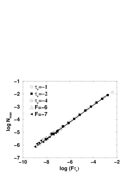
FIG. 7.: Dependence of the maximum island density $N_{max}$ on $F\tau_{e}$ in the direct impingement regime ($X_{S}\ll 1$). The solid line shows our prediction ($N_{max}\sim(F\tau_{e})^{2/3}$ for extremely low evaporation times, Eq.  69a). We see that our prediction remarquably fits the data over more than 6 orders of magnitude. The numbers indicate the values of logarithms of the evaporation time $\tau_{e}$ or the flux $F$ for the different sets of data.

4 Condensation coefficient at the maximum island density

A last test for the analysis is presented in Fig  8. We show that the dependence of the sticking coefficient S at the saturation island density ($S=\theta_{max}/Ft_{c}$) follows Eqs.  55, 44 and  65. By constructing an evaporation parameter $\eta=FX_{S}^{2}(1+X_{S}^{4})$, we can group all the regimes in a single curve : for the complete condensation regime, $S\sim\eta^{0}\sim 1$, for the others $S\sim\eta^{1/3}$.

FIG. 8.: Evolution of the sticking coefficient at the maximum island density as a function of the evaporation parameter $FX_{S}^{2}(1+X_{S}^{4})$. The solid lines represent our predictions (Eqs.  55 and  65). See the text for details.

D Island size distributions

Island size distributions have proven very useful as a tool for experimentalists to distinguish between different growth mechanisms [25, 32]. By size of an island, we mean its total number of monomers or mass. Unfortunately this information is beyond the reach of the simple mean field rate equation analysis presented above [9]. Nevertheless, the distributions can be obtained from the simulations. Fig  9 shows the evolution of the rescaled [7, 32] island size distributions as a function of the evaporation parameter $\epsilon={\left(1+X_{S}\right)}X_{S}^{5}\left(\frac{F}{D}\right)$. It is clear that the distributions are significantly affected by the evaporation, smaller islands becoming more numerous when evaporation increases. This trend can be qualitatively understood by noting that new islands are created continuously when evaporation is present, while nucleation rapidly becomes negligible in the complete condensation regime. The reason is that islands are created (spatially) homogeneously in the last case, because the positions of the islands are correlated (through monomer diffusion), leaving virtually no room for further nucleation once a small portion of the surface is covered ($\theta\sim 0.05$). In the limit of strong evaporation, islands are nucleated randomly on the surface, the fluctuations leaving large regions of the surface uncovered. These large regions can host new islands even for relatively large coverages, which explains that there is a large proportion of small ($s<s_{m}$) islands in this regime.

FIG. 9.: Rescaled island size distributions for different values of the evaporation parameter $\epsilon$ and different coverages $\theta$ between .05 and .2. $p(s/s_{m})$ represents the probability to find an island containing s monomers when the average size is $s_{m}=\theta/N$. If $n_{s}$ is the number of islands containing s monomers, we have $p(s/s_{m})=s_{m}*n_{s}/N_{t}$ where $N_{t}$ is the total number of islands. The solid line shows the size distribution obtained without evaporation. The first number next to each symbol corresponds to log $\epsilon$. The two other figures correspond to log $F$ and log $\tau_{e}$ respectively ($\tau=1$).

VI Discussion

Other authors have analyzed similar mean-field rate equations to find the growth dynamics and maximum island density in the presence of evaporation [15, 17, 18, 19]. In what follows, we discuss the relationship between our work and the preceding studies. In fact, a distinction must be made between the result of Stoyanov and Kaschiev, and that of Venables et al.

Stoyanov and Kaschiev consider that atoms may diffuse on top of an island, with the same diffusion length as on the substrate ($X_{S}=X_{S}^{*}$ in our notations). This corresponds to the regimes described by Equations  67 and  68a (they do not consider the direct impingement regime). However, their result in the regime where evaporation is important is $N_{max}\sim(F\tau_{e})^{1/2}$, different from our predictions (see both Eq.  68a and Eq.  69b), which are clearly supported by our simulations (see for example Fig.  5). As shown in the following, we think that the difference with our result stems from overlooking the fact that only the adatoms falling at a distance $X_{s}$ from the island edge contribute to the rate of growth of the island : in other terms, their capture cross section is not appropriate.

Stoyanov and Kaschiev assume, as we do, that the diffusing adatoms have two possible fates: either to evaporate or to be captured by an island. Their lifetime $\tau_{l}$ is thus

$$\frac{1}{\tau_{l}}=\frac{1}{\tau_{e}}+DN\;,$$ (70)

and the adatom density reads

$$\rho\approx F\tau_{l}\approx\frac{F\tau_{e}}{1+D\tau_{e}N}\;.$$ (71)

This is Eq. (6.2) of [19].

At this point, the incorrect assumption is made that the rate of growth of the area of an island of radius $R$ reads $d{R^{2}}/dt\approx D\rho\approx FD\tau_{e}/(1+D\tau_{e}N)$ throughout the strong evaporation regime (cf. Sec IV). Writing then

$$D\rho^{(i^{*}+1)}\approx\frac{dR^{2}}{dt}N^{2}\approx D\rho N^{2}\;,$$ (72)

one finds $\rho^{i^{*}}\approx N^{2}$, or

$$N^{2}(1+X_{s}^{2}N)^{i^{*}}\approx\left(\frac{F}{D}X_{s}^{2}\right)^{i^{*}}\;.$$ (73)

This is Eq. (6.12) of [19], and it leads to $N\approx(F/D)^{i^{*}/2}X_{s}^{i^{*}}$ in the “incomplete condensation”, $X_{s}^{2}N\ll 1$.

On the other hand, Venables et al. actually study (though it may not be easily guessed by reading their papers : we would like here to acknowledge an anonymous referee for precious help) the regime where all the particles deposited on top of the islands immediately fall on its border, thus contributing to increase its radius. This corresponds to the subregime described by Eq.  68b. Our prediction agrees with their result in the ”Extreme Incomplete” regime (see Table 1 of Ref. [18]). This regime applies only if diffusion and/or desorption are different on the substrate and on top of islands, which cannot be the case in homoepitaxial situations. In heteroepitaxial growth, on the other hand, the substrate and the islands of the first monolayer are chemically different, and Venables et al.’s assumption may apply; however, it is a special situation, not the general rule. The origin of their ”initially incomplete” regime is more mysterious. We try in the following to understand its origin.

We now show that the assumption of Venables et al.’s concerning the atoms falling on top of an island, leads to their equation for the maximum island density, Eq. (2.17) of Ref. [18]. In our notations the latter reads

$$N(1+X_{s}^{2}N)^{i^{*}}(\theta_{0}+X_{s}^{2}N)\approx(F/D)^{i^{*}}X_{s}^{4i^{*}}\;.$$ (74)

where $\theta=R^{2}N$ is the deposited dose (coverage) and $\theta_{0}$ its value at coalescence.

Assume that an island grows by capturing all atoms falling on top of it, plus those diffusing to it. Then, the rate of growth of the island area is

$$\frac{dR^{2}}{dt}\approx FR^{2}+D\rho\approx F\theta/N+D\rho\;,$$ (75)

where $\theta=R^{2}N$ is the deposited dose, or coverage.

From Eq. (71) and the nucleation rate, one finds

$$\frac{1}{\tau_{\rm nuc}}\approx D\rho^{i^{*}+1}\approx D\left(\frac{F\tau_{e}}{1+D\tau_{e}N}\right)^{i^{*}+1}\;.$$ (76)

Letting (76) equal to $(dR^{2}/dt)N^{2}$ (cf. Eq. 72), one has

$$D\left(\frac{F\tau_{e}}{1+D\tau_{e}N}\right)^{i^{*}+1}\approx F\theta_{0}N+D\frac{F\tau_{e}}{1+D\tau_{e}N}N^{2}\;,$$ (77)

where $\theta_{0}<1$ is the coverage at coalescence. Rewriting yields

$$\frac{(F/D)^{i^{*}}X_{s}^{4i^{*}}}{(1+X_{s}^{2}N)^{i^{*}}}\approx\left[\theta_{0}(1+X_{s}^{2}N)+X_{s}^{2}N\right]N\approx(\theta_{0}+X_{s}^{2}N)N\;,$$ (78)

which gives immediately Eq. (74).

We now turn on the relation of our crossover scaling (section III-C) to recent work by Bales [34]. Recently, the crossover scaling of the island density between different growth regimes on vicinal surfaces (without evaporation) was addressed by Bales [34], and by Pimpinelli and Peyla [33]. In particular, Bales claims that “when atoms desorb from the surface a crossover scaling form identical to” his results “is satisfied with” the distance between surface steps “replaced by the average distance $X_{s}$ a monomer will travel before desorbing” [34].

We argue that Bales’ claim is not true, as it stands. To see this, we need consider what happens on a vicinal substrate. We do this using the argument of Sect. III. Of course, competition between two length scales occurs in this case, too, the two lengths being the adatom diffusion length before capture by an island, $\ell_{s}$, and the step-step distance $\ell$. When $\ell_{s}\ll\ell$, the diffusing adatoms behave as though they were on a flat substrate, and the island density is still given by equation (4). In the opposite case, $\ell_{s}\gg\ell$, the adatom density is fixed by capture at steps, so that $\rho$ can be found by replacing $X_{s}$ by $\ell$ in Eq. (5), in agreement with Bales’ statement:

$$\rho\approx F\ell^{2}/D\;.$$ (79)

However, since evaporation is now neglected, an island grows by capturing all adatoms diffusing to its border. This means the island average radius grows as

$$R\approx\ell\sqrt{Ft}\;,$$ (80)

and since $R\approx\ell_{s}$ at $t=t_{c}$, one has

$$\frac{1}{t_{c}}\approx F\frac{\ell^{2}}{\ell_{s}^{2}}\approx F\ell^{2}N\;.$$ (81)

In the regime of dominant adatom capture by steps the island density at saturation is found from

$$D\rho^{i^{*}+1}\approx\frac{N}{t_{c}}$$ (82)

and thus

$${N}\approx\left(\frac{F}{D}\ell^{2}\right)^{i^{*}/2}\;.$$ (83)

A crossover between equation (4) and (83) is thus expected: it has been actually found by Pimpinelli and Peyla [33].

Bales [34] considered the crossover scaling of the island density at low coverage. His result for the regime of dominant adatom capture by steps, Eq. (9) of his paper, is found (within logs) by letting $t_{c}=t=\theta/F$ and $i^{*}=1$ in (82) above,

$${N}\approx\frac{F}{D}\ell^{4}\theta\;.$$ (84)

Note that this cannot be obtained by replacing $X_{s}$ by $\ell$ in our result, Eq. (7) above. It is however obtained by replacing $X_{s}$ by $\ell$ in Venables’ result. This is because Venables does not take into account the crucial phenomenon which occurs during evaporation–namely, that only the adatoms falling near or at the step edge can contribute to the island growth. To neglect this is correct within Venables’ assumptions, as well as on a vicinal surface without evaporation, where the latter mechanism is replaced by adatom capture by steps.

Our crossover scaling does not therefore coincide with Bales’, and Bales’ results [34] however modified do not describe homoepitaxial growth with desorption ($X_{S}=X_{S}^{*}$).

VII Summary and Perspectives

By combining different mean-field analysis and extensive computer simulations, we have shown that the presence of evaporation has important effects on the growth of submonolayer films. We have investigated the different regimes that arise when the growth parameters are varied, and predicted the behaviour of several experimentally accessible quantities such as the island size distributions, the maximum island density and the time at which this maximum is reached. In some cases, by measuring these last two quantities we can infer the values of both the evaporation and the diffusion times, which are difficult to obtain otherwise. For example, if the experiments are carried in the intermediate regime (and this can be checked from the sticking coefficient), by using Equations   68a and  55, we obtain $\tau=F^{2}\left(t_{c}N_{max}\right)^{3}$ and $\tau_{e}=t_{c}{N_{max}}^{2}$.

We have also shown that our model is more general than previous studies of growth in presence of evaporation.

Future directions of study should include more realistic hypotheses for a direct comparison with experiments [16]. In particular, we are presently extending our analysis to the case of three-dimensional growth (i.e. leading to cap-shaped islands) and the influence of defects on the surface which could act as nucleation centers.

We wish to thank M. Meunier and C. Henry for helpful discussions, Ph. Nozières for a critical reading of the manuscript and an anonymous referee for precious comments on the connection of our analysis with previous works.

e-mail addresses : jensen@dpm.univ-lyon1.fr, hernan@ce.ifisicam.unam.mx, pimpinelli@ill.fr

REFERENCES

- [1] See the special issue of Physics Today (February 1990); F. Capasso (ed) Physics of Quantum Electronic Devices (Springer-Verlag, 1990)
- [2] A.-L. Barabasi and H. E.Stanley, Fractal Concepts in Surface Growth (Cambridge University Press, 1995).
- [3] J. Villain and A. Pimpinelli Physique de la Croissance Cristalline (Eyrolles, 1995) (english edition to be published by Cambridge University Press, 1997)
- [4] P. Jensen, La Recherche 283 42 (1996)
- [5] J. Villain, A. Pimpinelli, L.-H. Tang, and D. E. Wolf, J. Phys. I France 2, 2107 (1992); J. Villain, A. Pimpinelli and D.E. Wolf, Comments Cond. Mat. Phys. 16,1 (1992)
- [6] L.-H. Tang, J. Phys. I France 3, 935 (1993)
- [7] J.W. Evans and M.C. Bartelt, J. Vac. Sci. Technol. A 12, 1800 (1994); J.G. Amar, F. Family, and P.-M. Lam, Phys. Rev. B 50, 8781 (1994). For a review, see ref [2] and [3].
- [8] P. Jensen, A.-L. Barabási, H. Larralde, S. Havlin, and H. E. Stanley, Nature 368, 22 (1994); Physica A 207, 219-227 (1994); Phys. Rev. B 50, 15316 (1994)
- [9] G.S. Bales and D.C. Chrzan, Phys. Rev. B 50, 6057 (1994)
- [10] Y. W. Mo, J. Kleiner, M.B. Webb and M.G. Lagally, Phys. Rev. Lett. 66, 1998 (1991).
- [11] H. Röder, E. Hahn, H. Brune, J.-P. Bucher, and K. Kern, Nature 366, 141 (1993); H. Brune, C. Romainczyk, H. Röder, and K. Kern, Nature 369, 469 (1994); H. Brune, H. Röder, C. Boragno, and K. Kern, Phys. Rev. Lett. 73, 1955 (1994)
- [12] R. Q. Hwang, J. Schröder, C. Günther and R. J. Behn, Phys. Rev. Lett. 67, 3279 (1991); T. Michely, M. Hohage, M. Bott, and G. Comsa, Phys. Rev. Lett. 70, 3943 (1993)
- [13] C. Ratsch, A. Zangwill, P. Smilauer and D Vvedensky, Phys. Rev. Lett. 72, 3194 (1994)
- [14] V. N. E. Robinson and J. L. Robins, Thin Solid Films, 12, 255 (1972);
- [15] M. J. Stowell, Phil. Mag. 26, 361 (1972)
- [16] M. Meunier, PhD thesis (Université Aix-Marseille, 1995); M. Meunier and C.R. Henry, Surf. Sci. 307, 514 (1994)
- [17] J. A. Venables, Phil. Mag. 27, 697 (1973)
- [18] J. A. Venables, G. D. T. Spiller, and M. Hanbücken, Rep. Prog. Phys. 47, 399 (1984).
- [19] S. Stoyanov and D. Kaschiev, Current Topics in Mat. Science, Ed. E. Kaldis, (North-Holland, 1981)
- [20] P. Jensen, A.-L. Barabási, H. Larralde, S. Havlin, and H. E. Stanley, Fractals (to be published, 1996)
- [21] P. Jensen, L. Bardotti, A.-L. Barabási, H. Larralde, S. Havlin, and H. E. Stanley, MRS Proceedings 407 (Fall 1995 Meeting).
- [22] For recent experimental results, see for example Evolution of Epitaxial Structure and Morphology, ed. A. Zangwill, D. Jesson, D. Chambliss and R. Clarke, or Disordered Materials and Interfaces - Fractals, Structure and Dynamics, ed. H.E. Stanley, H.Z. Cummins, D.J. Durian and D.L. Johnson, both Proceedings of the Materials Research Society, Fall Meeting, Boston, December 1995, volumes 399 and 407 respectively .
- [23] Proceedings of the 14th European Conference on Surface Science (September 1994), Surface Science 331-333 (1995).
- [24] R. L. Schwoebel, J. Appl. Phys. 40, 614 (1969); R. L. Schwoebel and E. J. Shipsey, J. Appl. Phys. 37, 3682 (1966); J. Villain, J. Physique I 1, 19 (1991)
- [25] L. Bardotti, P. Jensen, M. Treilleux, B. Cabaud and A. Hoareau, Phys. Rev. Lett. 74, 4694 (1995) ; L. Bardotti et al. (to be published, 1996).
- [26] P. Melinon et al. Int. J. of Mod. Phys. B 9, 339-397 (1995)
- [27] G.L. Kellogg, Phys. Rev. Lett. 73, 1833 (1994) and references therein.
- [28] T. J. Raeker and A. E. DePristo, Surf. Sci. 317, 283 (1994)
- [29] S. Liu, L. Bönig and H. Metiu, Phys. Rev. B 52 2907 (1995)
- [30] M. C. Bartelt, S. Gunther, E. Kopatzi, R. J. Behm and J. W. Evans (to be published, Phys Rev B, 1996)
- [31] G. Zinsmeister, Vacuum 16, 529 (1966); Thin Solid Films 2, 497 (1968); Thin Solid Films 4, 363 (1969); Thin Solid Films 7, 51 (1971)
- [32] J. A. Stroscio and D. T. Pierce, J. Vac. Sci. Technol. B 12 1783 (1994)
- [33] A. Pimpinelli and P. Peyla, in press on International Journal of Modern Physics B.
- [34] G.S. Bales, Surface Sci. 356, L439 (1996).