Multifractal analysis of the metal-insulator transition in anisotropic systems

Abstract

We study the Anderson model of localization with anisotropic hopping in three dimensions for weakly coupled chains and weakly coupled planes. The eigenstates of the Hamiltonian, as computed by Lanczos diagonalization for systems of sizes up to $48^{3}$, show multifractal behavior at the metal-insulator transition even for strong anisotropy. The critical disorder strength $W_{c}$ determined from the system size dependence of the singularity spectra is in a reasonable agreement with a recent study using transfer matrix methods. But the respective spectrum at $W_{c}$ deviates from the “characteristic spectrum” determined for the isotropic system. This indicates a quantitative difference of the multifractal properties of states of the anisotropic as compared to the isotropic system. Further, we calculate the Kubo conductivity for given anisotropies by exact diagonalization. Already for small system sizes of only $12^{3}$ sites we observe a rapidly decreasing conductivity in the directions with reduced hopping if the coupling becomes weaker.

I Introduction

It is well known that the three dimensional (3D) isotropic Anderson model exhibits a metal-insulator transition (MIT): Increasing the disorder of the random potential site energies causes the wave functions to localize. [1] There exists a mobility edge in the energy-disorder diagram which separates extended from localized eigenstates. In order to determine these critical disorders $W_{c}(E)$ accurately, the transfer-matrix method (TMM) together with the one-parameter finite-size scaling hypothesis applied to quasi-1D bars has been used with much success in the past. [2, 3, 4] Recently, the anisotropic Anderson model has received much attention in connection with the anisotropic transport properties of the high $T_{c}$ cuprates and a possible contradiction to the scaling theory of localization was mentioned[5] supported by a diagrammatic analysis. [6] However, recent TMM studies[7, 8, 9] show that the one-parameter scaling theory is still valid and further that an MIT exists even for strong hopping anisotropy $\gamma$. The values of the critical disorder in the band center were found to follow a power law $W_{c}\propto(1-\gamma)^{\beta}$ independent of the orientation of the quasi-1D bar. $\beta$ was argued to be independent of the strength of the anisotropy.

Here, we shall study the problem of Anderson localization by a different method: we focus our attention directly on the eigenfunctions of the Hamiltonian. In an infinite system the wave functions are expected to be localized on the insulating side and extended on the metallic side even arbitrarily close to the transition. As first suggested by Aoki[10] the fractal nature of the critical eigenstates can connect these discrepant characteristics. Indeed, large fluctuations of the wave functions have been observed numerically which dominate — at least at small length scales — the character of the states and invalidate the simple notions of exponentially localized or homogeneously extended states. Approaching the transition these fluctuations increase and at the critical disorder they are expected to occur on all length scales. It has been shown[11] that such wave functions are multifractal entities. To characterize the eigenstates of the isotropic Anderson model the singularity spectrum $f(\alpha)$ has been used successfully.[11] A characteristic spectrum $f_{c}(\alpha)$ was shown to determine the mobility edge independent of the microscopic details of the sample.[12] Further, around its maximum, $f_{c}(\alpha)$ agrees well with an analytical result of Wegner[13] based on a nonlinear $\sigma$ model calculation. Near the critical disorder $W_{c}$, characteristic changes of $f(\alpha)$ were observed when the system size was increased.[14] These distinguish the localized and the extended character of the states and therefore allow us to determine the transition directly from multifractal properties of eigenstates.

It is our aim in the present work to use and extend these concepts for the case of anisotropic hopping. In Sec. II we introduce our notation and define the anisotropies of weakly coupled planes and weakly coupled chains. We next recall the concepts and methods of the multifractal analysis employed in the sequel. Using the hypothesis of a characteristic singularity spectrum, we estimate the critical disorders in Sec. IV B. To check the validity of the hypothesis we analyze the system size dependence of the multifractal properties and compare our results with TMM data.[8, 9] For completeness, we also study the conductivity of small samples of anisotropic systems in Sec. V. We discuss our results in Sec. VI.

II The Anderson model with anisotropic hopping

The Anderson Hamiltonian is given as[1]

$$H=\sum_{i}\epsilon_{i}|i\rangle\langle i|+\sum_{i\neq j}t_{ij}|i\rangle\langle j|\quad.$$ (1)

Here, the sites $i=(x,y,z)$ form a regular cubic lattice of size $N^{3}$ and the potential site energies $\epsilon_{i}$ are as usual taken to be randomly distributed in the interval $[-W/2,+W/2]$. The transfer integrals $t_{ij}$ are restricted to nearest neighbors and depend only on the spatial direction, so $t_{ij}$ can either be $t_{x}$, $t_{y}$ or $t_{z}$. We set the energy scale by normalizing the largest $t_{ij}$ to $1$.

Following Ref. [8], we study two possibilities of anisotropic transport: (i) weakly coupled planes with $t_{x}=t_{y}=1$, $t_{z}=1-\gamma$ and (ii) weakly coupled chains with $t_{x}=t_{y}=1-\gamma$, $t_{z}=1$. Here the parameter $\gamma\in[0,1]$ describes the strength of the anisotropy. Hence, for $\gamma=0$ we recover the isotropic 3D case and $\gamma=1$ corresponds to $N$ independent planes or $N^{2}$ independent chains. The direction with normal (reduced) transfer integral is called the parallel (perpendicular) direction.

The Lanczos algorithm,[15] which is well suited for the diagonalization of sparse matrices, allows us to solve the eigenvalue equation $H\Psi(E)=E\Psi(E)$ for system sizes up to $N=72$, yielding eigenvalue/eigenvector pairs in a requested energy range. We use state-of-the-art workstations and a parallel computer with 128 PowerPC processors. It takes about 11 hours to diagonalize the Anderson Hamiltonian with $N=48$ on the parallel machine using 8 processors. The workstations need about 35 hours for the same calculation. Since we also have to perform a statistical averaging over different disorder configurations, we have restricted the systematic investigations to sizes up to $N=48$. In order to allow a direct comparison with the results of Refs. [7, 8, 9], we restrict our study to the states in the center of the band such that $E=0$. Numerically this is the worst case because of the high density of states there which requires a very large tridiagonal matrix in the Lanczos algorithm to determine the eigenvalues.

III Multifractal analysis

Fractal measures are widely used in physics to characterize objects such as percolating clusters, random walks, and random surfaces. [16, 17, 18] The common geometric feature of such point sets is the self-similarity: Parts of the set are similar to the whole, at least in a statistical sense. However, for fluctuating physical quantities such as the probability amplitude of an eigenstate $\Psi(E)$ of the Anderson model, the appropriate concept is given by the multifractal measures: If the mentioned fluctuations are statistically the same on every length scale, i.e., if all the moments of the investigated quantity are self similar, the object is (statistically) self-affine and is called a multifractal.

A characteristic property of multifractals is their singularity spectrum $f(\alpha)$.[18] Let us briefly describe an algorithm to determine this quantity, based on the standard box counting procedure: We consider a volume $L^{D}$ in our $D$ dimensional space which contains the support of the physical variable, i.e., all points where the variable is defined. We cover it with a number of ”boxes” of linear size $r=\delta L$. The actual shape of the boxes is not important, they may be spheres as well. Next, we determine the contents $\mu_{i}(\delta)$ of each box $i$ by summing or integrating the investigated quantity over the part of the support inside the box. For a self-affine object one finds a power-law dependence $\mu_{i}(\delta)\propto\delta^{\alpha_{i}}$ in the limit $\delta\to 0$. The so-defined singularity strength $\alpha_{i}$ is assigned to each point of the support. The subset $S_{\alpha}$ which contains all points with the same value of $\alpha$ is a fractal with fractal dimension $f(\alpha)$ defined by $K(\alpha,\delta)\propto\delta^{-f(\alpha)}$. Here, $K(\alpha,\delta)$ is the number of boxes which cover $S_{\alpha}$. A multifractal object consists of a (infinite) number of subsets $S_{\alpha}$ with different fractal dimensions.

In the present work we shall use an equivalent but numerically more convenient algorithm to compute the singularity spectrum. Our physical quantity is again the probability amplitude of eigenstates. Considering the normalized $q$th moments of the box probability $\mu_{i}(q,\delta)=\mu_{i}^{q}(\delta)/\sum_{k}\mu_{k}^{q}(\delta)$ it is possible to find[19] a parametric expression of $f(\alpha)$ such that

$$\begin{array}[]{l}\alpha(q)=\lim_{\delta\to 0}\sum_{i}\mu_{i}(q,\delta){\rm ln}\mu_{i}(1,\delta)/{\rm ln}\delta\quad,\\ f(q)=\lim_{\delta\to 0}\sum_{i}\mu_{i}(q,\delta){\rm ln}\mu_{i}(q,\delta)/{\rm ln\delta}\quad.\end{array}$$ (2)

We plot the sums in (2) versus ${\rm ln}\delta$ and observe multifractal behavior if and only if the data may be well fitted by straight lines. The slope from the linear regression procedure used in the fit gives $f$ and $\alpha$. Note, that a check of the linearity is important, since the numerical procedure gives an $f(\alpha)$ curve for nearly every distribution of the physical variable, but without the mentioned linearity it does not indicate multifractality.

In general, $f(\alpha)$ is a nonnegative, convex function with $0<\alpha_{min}\leq\alpha\leq\alpha_{max}<\infty$. The maximum of $f(\alpha)$ at $\alpha(q=0)\equiv\alpha_{0}$ equals the dimension of the support, i.e., the fractal dimension $D_{f}$ of the subset of points where the investigated quantity is not zero. For our wave functions $D_{f}=D=3$ because they are nowhere exactly zero. The whole $f(\alpha)$ curve is below the bisector $f(\alpha)=\alpha$ except at $\alpha(q=1)\equiv\alpha_{1}$ where both curves touch. For $q=1$ the relation $f(\alpha_{1})=\alpha_{1}$ is fulfilled. $\alpha_{1}$ equals the entropy dimension or information dimension and one can show that the corresponding set $S_{\alpha_{1}}$ contains the entire measure.[18]

There are two limits which will be important for the later interpretation of our results. Consider a D-dimensional support. (i) A uniform distribution is represented by the single point $f(\alpha=D)=D$ in the singularity spectrum, because $\mu_{i}(\delta)\propto(L\delta)^{D}$ for every point of the support. (ii) With increasing localization the spectrum becomes wider and an extremely localized distribution with measure $1$ at one point and $0$ elsewhere has a spectrum which consists of two points only: $f(\alpha=0)=0$ and $f(\alpha=\infty)=D$. This is because the box around the maximum has contents $1$ for each $\delta$, so $\alpha$ is $0$ for this single point while all other points have $\mu_{i}\propto\delta^{\infty}=0$. In Fig. 1 we show two typical singularity spectra of 3D wave functions corresponding to a localized and an extended wave function. The tendency towards the 2 limiting cases can be seen for these two examples already: The extended state has a narrow $f(\alpha)$ curve close to $f(3)=3$ while the localized wave function is represented by a very wide spectrum with larger $\alpha_{0}$ and smaller $\alpha_{1}$.

IV Calculation of critical disorders $W_{c}(\gamma)$

A Existence of multifractal eigenstates

As has been shown in Refs. [8, 9] by the TMM, the anisotropic Anderson model still exhibits a MIT for all $\gamma>0$ in the band center $E=0$ and, by the general arguments given above, we expect the wave functions at the transition point to be multifractals just as in the isotropic case. As a check we have computed various eigenstates close to the proposed[8, 9] critical disorders $W_{c}$ for system sizes up to $N=48$. In Fig. 2, we show the data for the linear regression of a typical state with $W\approx W_{c}$. We find even for very strong anisotropies $\gamma=0.99$ that the sums in Eq. (2), plotted versus ${\rm ln}\delta$ are linear. Therefore, we do find multifractal behavior of the wave functions close to the critical disorder for the anisotropic Anderson model.

Every singularity spectrum is characteristic only for the particular configuration of the site energies. But for a given set of parameters $\{W,E,\gamma\}$ the different $f(\alpha)$ curves fluctuate around one singularity spectrum. In order to suppress these statistical fluctuations we average the spectra obtained from $3$ to $8$ eigenstates close to $E=0$ for 12 realizations of the random site energies. The averaged spectrum is thus characteristic for the set of parameters $\{W,E,\gamma\}$ and will be used in the next sections to compute the critical disorder $W_{c}$ as a function of the anisotropy $\gamma$.

B Estimation of $W_{c}$ from comparison with the characteristic spectrum

In the isotropic case a characteristic singularity spectrum $f_{c}(\alpha)$ was found previously[20] at all points of the mobility edge independent of the microscopic details of the system such as the probability distribution of the site energies. The region close to the maximum of $f_{c}(\alpha)$ is described well by an analytical result of Wegner[13] from the $2+\varepsilon$ expansion of the non-linear $\sigma$ model, i.e.,

$$f_{c}(\alpha)=D-\frac{\varepsilon}{4}\left(\frac{D-\alpha}{\varepsilon}+1\right)^{2}+O(\varepsilon^{4})\stackrel{{\scriptstyle\varepsilon=1}}{{\approx}}3-\frac{(4-\alpha)^{2}}{4}.$$ (3)

As a hypothesis we shall now assume that this characteristic spectrum determines the transition even in the case of anisotropic hopping. This hypothesis is certainly valid in the limit $\gamma\to 0$ but needs further support for larger anisotropies.

We find that for each anisotropy $\gamma$ there exists a corresponding $W_{f_{c}}$ such that the eigenstates are characterized by $f_{c}$. Identifying $W_{c}=W_{f_{c}}$ gives us an estimate for the $\gamma$ dependence of the critical disorder. Note that since the singularity spectrum should be independent of the system size at the transition point, it is sufficient to investigate small systems. We have used systems with $N=24$ for the results presented in this section.

1 Weakly coupled planes

Assuming the validity of $f_{c}$ we find a crossover between two power laws in the $\gamma$ dependence of the critical disorder: $W_{c}=55(1-\gamma)^{0.86}$ for $\gamma\geq 0.9$ and $W_{c}=16.8\,(1-\gamma)^{0.35}$ for $\gamma\leq 0.9$ as can be seen in Fig. 3. This does not agree with the results of Ref. [8], where $\beta=0.25$ has been calculated within the self-consistent theory of localization and where the single power law $W_{c}=15.4(1-\gamma)^{0.25}$ has been deduced from the TMM data.

2 Weakly coupled chains

In Fig. 4 the results for $W_{c}(\gamma)$ for weakly coupled chains are shown. Using $f_{c}$ we find $W_{c}=17.6(1-\gamma)^{0.74}$ which is very similar to the TMM data[9] $W_{c}=16.19(1-\gamma)^{0.611}$. The difference becomes significant only for very large $\gamma\gtrsim 0.9$. The exponent $\beta=0.611$ was obtained from a fit of the TMM data over the whole $\gamma$ range. For large $\gamma$ the authors of Ref. [9] get $\beta=0.5$. This is consistent with the result of Ref. [8].

C Estimation of $W_{c}$ from the system-size dependence

We have shown in the last section, that the assumption of the characteristic $f_{c}$ leads to large differences in the estimates of $W_{c}$ between the TMM results [8, 9] and our results based on the multifractal analysis. Thus we will now use a more direct method to estimate $W_{c}(\gamma)$ from the multifractal properties of the eigenstates. From the isotropic case it is known[12] that multifractal behavior is found not only directly at the critical disorder $W_{c}$ but also close to the transition. The reason is the finite sample size which is much smaller than the characteristic length scales of the states close to $W_{c}$. In this range the exponential decay or uniformly extended character of the wave function is masked by large fluctuations and it is not obvious to which side of the MIT a given state belongs. Due to the relatively small sample size the system is very sensitive to its boundary. Correspondingly, a characteristic change in the singularity spectrum is observed when the system size is increased. This change can be evaluated to distinguish the localized or extended character of the wave function. For an extended state the $f(\alpha)$ curve becomes narrower and the maximum position is shifted towards smaller values of $\alpha$, approaching the value 3. The opposite behavior is found for a localized state. Thus the spectra tend towards the extreme cases discussed in Sec. III. Indeed we expect these limiting cases, namely $f(3)=3$ for the metallic side and $f(0)=0$ and $f(\infty)=3$ for the insulating side, to be reached for infinitely large system size for any disorder except $W_{c}$. Only directly at the transition the wave functions are multifractal, the fluctuations are the same on all length scales, and $f(\alpha)$ is independent of the system size. This makes is feasible to determine the critical disorder by analyzing the system-size dependence of the singularity spectra.[14]

1 Weakly coupled planes

We show in Fig. 5 an example of weakly coupled planes with $\gamma=0.8$. The above described different behaviors of the spectra can be seen. For $W=8$, a larger system size results in a narrower $f(\alpha)$ curve which is characteristic for extended states. On the other hand, the increase in the system size for $W=12$ yields a widening of the spectrum indicating localized states. The singularity spectrum for $W=10$ is least effected by the change of the system size and we thus conclude a critical disorder $W_{c}(\gamma=0.8)=10\pm 1$. Considering the error bars, the $f(\alpha)$ curve for $W_{c}$ equals the characteristic spectrum $f_{c}$ of the isotropic case. For moderate anisotropies $\gamma\lesssim 0.8$ this confirms the hypothesis of a characteristic $f_{c}$.

Visual observation of the system-size dependence of the $f(\alpha)$ curves is not well suited for a systematic search for the transition. A better method is to focus attention to special points of the spectra such as the position $\alpha_{0}$ of the maximum and the information dimension $D_{1}=\alpha_{1}$. An increase of the system size causes a decreasing $\alpha_{0}$ and a increasing $\alpha_{1}$ for extended states and the opposite tendency for localized states[14, 21] as described in Sec. III. A constant behavior of $\alpha_{0}$ and $\alpha_{1}$ versus system size indicates $W_{c}$. Following Ref. [14] we have parameterized the system-size dependence by $1/{\rm ln}(N)$ which has been found to give a nearly linear behavior of $\alpha_{0}$ and $\alpha_{1}$ thus distinguishing their tendencies more clearly.[14, 21, 22] In Fig. 6 we find a constant behavior at the same value of the disorder for both quantities and we conclude $W_{c}(\gamma=0.96)=8.0\pm 0.5$.

For very weakly coupled planes we get significantly larger values of $W_{c}$ than in Sec. IV B. The new values are close to, but slightly larger than the TMM data[8] as can be seen in Fig. 3. Our data follow $W_{c}=16.3(1-\gamma)^{0.25}$ which confirms the exponent $\beta=0.25$ derived analytically.[8] We therefore conclude that $f_{c}$ is no longer characteristic for the eigenstates at the MIT for weakly coupled planes with $\gamma\gtrsim 0.8$. In our present analysis we find wider singularity spectra which is a sign of a tendency towards localization. An eigenstate at the transition for very strong anisotropy $\gamma=0.99$ is shown in Fig. 7. The probability amplitude is concentrated to a few planes perpendicular to the direction with reduced transfer. This coincides with the observation that the localization length is smaller by a factor $1-\gamma$ in the perpendicular direction compared with the parallel one.[8] In the mentioned planes the wave function looks like a fractal with holes and islands of different sizes, very similar to the critical eigenstates of the isotropic system. It may well be that the cubic boxes used in the box-counting procedure for the multifractal analysis cannot appropriately measure this fractal, because most box sizes exceed the number of planes on which the wave functions are concentrated. Therefore it is possible that the deviations of $W_{f_{c}}$ from $W_{c}$ in Fig. 3 are an artefact of the analysis.

2 Weakly coupled chains

The results for the $W_{c}(\gamma)$ dependence of weakly coupled chains are shown in Fig. 4. They are in reasonable agreement with the TMM data, [9] although we cannot reproduce the exponent[8] $\beta=0.5$. The differences between $W_{c}$ and $W_{f_{c}}$ are not as large as in the other case and the multifractal properties of the critical states are therefore similar to those of the isotropic system.

V Conductivity in small anisotropic systems

The transport properties are determined by the localization properties of the states. At $T=0$ localized states cannot contribute to charge transfer and we have insulating behavior. On the other hand, extended states yield metallic behavior. The Kubo formula following from Fermi’s golden rule provides a connection of the electrical conductivity and the electronic states $|n\rangle$.

Let us consider an electrical AC field with frequency $\omega=\hbar E$ in $x$ direction on an sample with volume $N^{3}$. We assume a half-filled band at $T=0$ such that all states with $E\leq 0$ are occupied while all others are unoccupied. A configuration average because of the random site energies is denoted by $\left\langle\,\right\rangle_{C}$. Neglecting prefactors the real part $\sigma$ of the conductivity is given by[23]

$$\sigma(E)\sim\left\langle\sum_{nn^{\prime}}|\langle n|x|n^{\prime}\rangle|^{2}E_{nn^{\prime}}\delta(E-E_{nn^{\prime}})\right\rangle_{C}\quad,E\neq 0\quad.$$ (4)

In order to compute this quantity it is necessary to know all eigenvalues and all eigenstates. We use the standard Householder algorithm to diagonalize the Hamiltonian (1). We average over 90 to 150 configurations to suppress the large statistical fluctuations of $\sigma$. This limits the treatable linear system size to $N=12$. As a consequence we encounter strong finite-size effects for $W\leq 4$. The small number of eigenenergies in the ordered limit is not smeared out sufficiently by the disorder to yield a smooth density of states $\rho(E)=\frac{1}{N^{3}}\left\langle\sum_{n}\delta(E-E_{n})\right\rangle_{C}$ as shown in Fig. 8 for $W=1$ and $\gamma=0.9$. We also note that the density of states for larger disorder values and $\gamma\geq 0.9$ agrees with that of the respective 1D or 2D system within the uncertainty due to fluctuations. However, the transport behavior of the states is completely different: In 1D and 2D there is no MIT ($W_{c}=0$) while 3D systems exhibit an MIT even for very strong anisotropy as shown in Sec. IV.

Because the characteristic length scales of the wave functions exceed the system size it is a priori not clear whether the localization behavior of the states has any measurable influence on the computed conductivity. Suppose there is no such influence, then the matrix elements $\langle n|x|n^{\prime}\rangle$ are all be equal and the conductivity is given by the $E$-weighted joint density of states $\sigma_{u}(E)=\left\langle\sum_{nn^{\prime}}E_{nn^{\prime}}\delta(E-E_{nn^{\prime}})\right\rangle_{C}$. We compare $\sigma$ and $\sigma_{u}$ for weakly coupled planes with, e.g. $W=1$ and $\gamma=0.9$ in Fig. 9. The peak structure for this small disorder is a again finite size effect reflecting the peaks of $\rho(E)$. The positions of the minima of $\sigma(E)$ are the same as expected from the joint density of states but the minima are much more pronounced. The reason for this behavior is the strong localization of the states for energies with low $\rho(E)$ similar to the localization in the band tails; the latter causes the decrease of $\sigma$ at higher energies. Thus despite the small system size the conductivity is highly influenced by localization effects.

In Fig. 10 we present the conductivity computed for the two nonequivalent directions: parallel (a), (c) and perpendicular (b), (d) to the planes and chains, respectively. For strong anisotropy the wave functions are concentrated to a few chains or planes as shown in Fig. 7. Consequently, the conductivity is drastically reduced in the perpendicular direction. For $\gamma=0.9$ the maximum of $\sigma$ is reached at small energies because the most extended eigenstates appear in the band center. This causes the (small) peak for $W=1$. For strong disorder $W=15$ all eigenstates are strongly localized and the perpendicular conductivity is nearly negligible. For the parallel conductivity we find an increase if the anisotropy becomes stronger. Here, the transport is not handicapped by the anisotropic localization of the wave functions. The increase is relatively small for the planes and considerable for the chains. A good argument to explain this difference is the form of the density of states which yields a higher amount of possibly transitions for the energies around the position of the maximum of $\sigma(E)$ for the second. The parallel conductivity at $W=15$ is relatively small but considerable in a large energy range which reflects the disorder widened energy band. We note that the conductivities for a very strong anisotropy $\gamma=0.99$ are nearly equal to those of $\gamma=0.9$ in the parallel direction and again negligible in the perpendicular direction.

VI Conclusions

In the present work we have studied the localization behavior of eigenfunctions and transport properties of the Anderson model with anisotropic hopping. As expected from the general argument for the fractal nature of wave functions at the metal-insulator transition, multifractal eigenstates were found even for strong anisotropy. The multifractal description holds not only directly at the transition but also close to it due to the small system sizes considered. As a first estimate for the critical disorder $W_{c}$ we determined that $W_{f_{c}}$ where the states show the characteristic singularity spectrum $f_{c}(\alpha)$ which indicates the MIT in the isotropic case. But especially for weakly coupled planes the computed anisotropy dependence of the critical disorder differs remarkably from the TMM results. [8] We also analyzed the system-size dependences of the singularity spectra to determine the MIT. The observed $W_{c}(\gamma)$ agree reasonably well with the TMM data.[8, 9] Therefore we conclude that the ”characteristic spectrum” is no longer valid if the anisotropy becomes strong. This is surprising because $f_{c}$ was independent of the microscopic details of the isotropic system for the 3D case. The spectrum at $W_{c}$ for weakly coupled planes is wider than $f_{c}$. This coincides with the observed concentration of the probability amplitude to only a few planes perpendicular to the direction with reduced hopping for large anisotropy.

We have also studied the AC conductivity of small anisotropic samples using Kubo’s formula. In this case the treatable system sizes are very small because all eigenvalues and eigenvectors of the Hamiltonian are needed. Nevertheless we observe a rapidly decreasing conductivity in the direction with smaller hopping integral if the anisotropy becomes stronger. This is a pure localization effect. For the used small system size $N=12$ it is surprising that this can be observed, because the characteristic length scales are much larger for nearly all of the states. Another interesting fact is that the density of states for an anisotropy $\gamma=0.9$ is already nearly identically with that of the corresponding lower-dimensional system.

FIG. 1.: Singularity spectra of a localized ($W=1$) and an extended ($W=25$) state of an isotropic system with $N=48$. The circles ($\circ$) mark $f(\alpha_{0})$ and the squares ($\Box$) mark $f(\alpha_{1})$.

FIG. 2.: Linear regression data for the evaluation of Eq. (2) determining $\alpha(q)$ and $f(q)$ for weakly coupled planes with $\gamma=0.9$, $N=48$, $W=9$ and $q=-2(\circ),-1(\Box),0(\Diamond),1(\triangle),2(+)$.

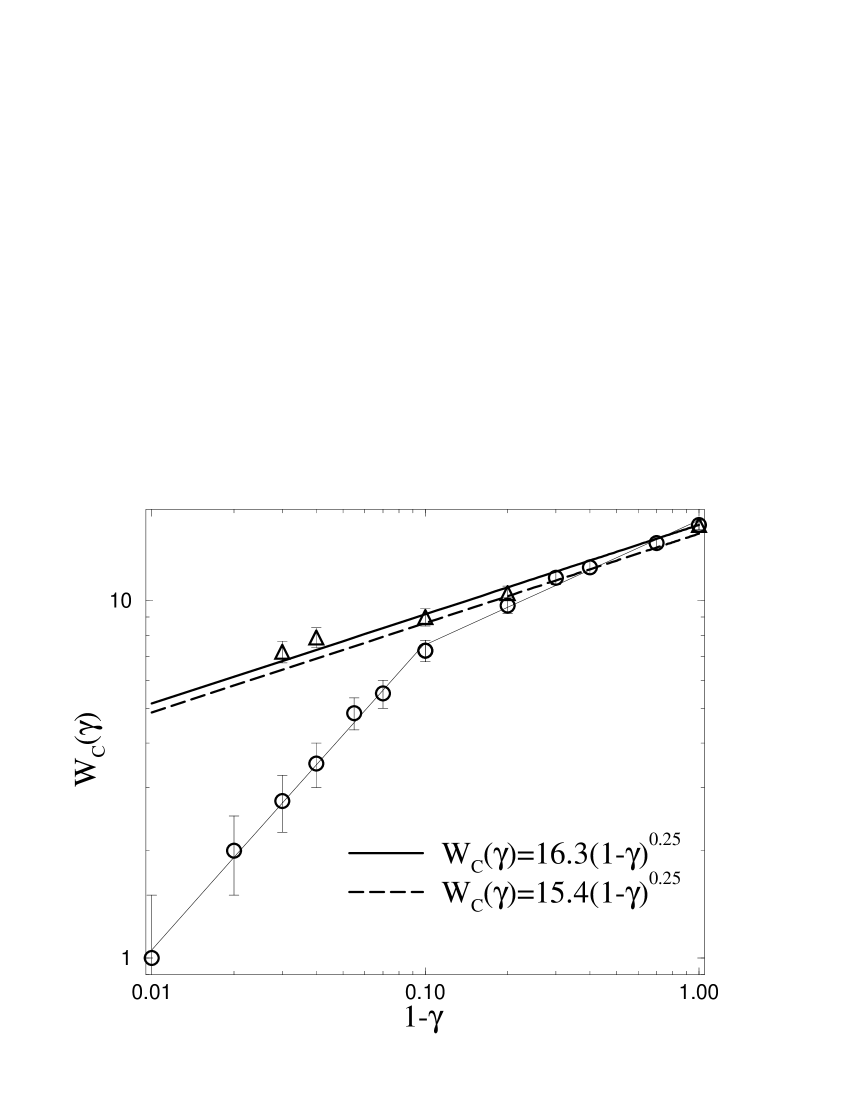
FIG. 3.: $W_{c}(\gamma)$ for weakly coupled planes as obtained from the “characteristic spectrum” ($\circ$) and from the system size dependence ($\triangle$). The thin solid lines represent the two power law fits to the ($\circ$) data. The thick dashed line is the result of Ref. [8]. The thick solid line is a combination of the isotropic result[4] $W_{c}=16.3$ and the perturbative exponent[8] $\beta=0.25$ which fits the ($\triangle$) data well.

FIG. 4.: $W_{c}(\gamma)$ for weakly coupled chains as obtained from the “characteristic spectrum” ($\circ$) and from the system size dependence ($\triangle$). The thin solid line is a power law fit to the ($\circ$) data, the thick dashed line is the result of Ref. [9]. The thick solid line is the combination of the isotropic result [4] $W_{c}=16.3$ and the perturbative exponent [8] $\beta=0.5$.

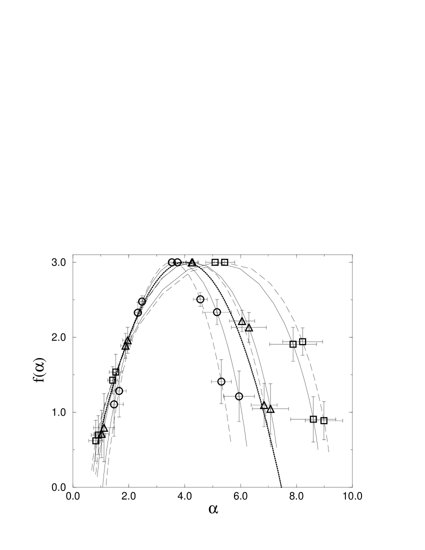
FIG. 5.: Singularity spectra for weakly coupled planes at $\gamma=0.8$ for the two system sizes $N=18\,(-)$ and $N=42\,(-\,-)$. The symbols distinguish $W=8(\circ),10(\triangle),12(\Box)$ and indicate $\alpha(q)$ and $f(q)$ for $q=-2,-1,0,1,2$ (from right to left). The error bars result from the linear regression (cp. Fig. 2) and the average over the different eigenstates (cp. Sec. IV A). The dotted line is the ”characteristic spectrum” $f_{c}$.

FIG. 6.: $N$ dependence of $\alpha_{0}$ and $\alpha_{1}$ for weakly coupled planes with $\gamma=0.96$ and $W=5.5(\circ),6.5(\Box),7.5(\star),8.5(\diamond),9.5(\triangle),10.5(+)$.

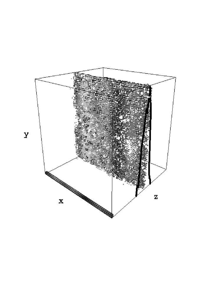
FIG. 7.: Wave function close to the MIT for very weakly coupled planes with $\gamma=0.99$, $N=48$ and $W=4.5$. Every site with probability $|\Psi_{i}|^{2}$ larger than the average $N^{-3}$ is shown as a box with volume $|\Psi_{i}|^{2}\times N$. The 764 cubes with $|\Psi_{i}|^{2}\times N>\sqrt{1000}$ are plotted in white with black edges. The grey scale distinguishes between different slices of the system along the x-axis. The thick solid line is the logarithm of the summed probability amplitude for each plane perpendicular to the z-axis. Again only values above $N^{-3}$ are shown.

FIG. 8.: Density of states for weakly coupled chains (a) and planes (b) with $\gamma=0.9$ and $N=12$. The data for $W=5$ and $15$ agree with that of uncoupled chains or planes within the statistical fluctuations. The peak structure for $W=1$ is due to the small system size.

FIG. 9.: Comparison of $\sigma$ and $\sigma_{u}$ in weakly coupled planes with $W=1$, $\gamma=0.9$, and $N=12$. $\sigma_{u}$ has been scaled to the same maximum value as $\sigma$.

FIG. 10.: Conductivity $\sigma$ for $N=12$ and various anisotropies $\gamma$ and disorders $W$ for weakly coupled chains (c), (d) and planes (a), (b) for the parallel (a), (c) and perpendicular (b), (d) direction. The perpendicular conductivity for $\gamma=0.9$ and $W=15$ is negligible while the parallel conductivity for $\gamma=0.9$ and $W=1$ exceeds the range of the diagram (see Fig. 9).

- [1] P. W. Anderson, Phys. Rev. 109, 1492 (1958).
- [2] A. MacKinnon and B. Kramer, Z. Phys. B 53, 1 (1983).
- [3] B. Kramer, A. Broderix, A. MacKinnon, and M.Schreiber, Physica A 167, 163 (1990).
- [4] B. Kramer and A. MacKinnon, Rep. Prog. Phys. 56, 1469 (1993).
- [5] A. G. Rojo and K. Levin, Phys. Rev. B 48, 16861 (1993).
- [6] A. A. Abrikosov, Phys. Rev. B 50, 1415 (1994).
- [7] Q. Li, C. M. Soukoulis, E. N. Economou, and G. S. Grest, Phys. Rev. B 40, 2835 (1989).
- [8] I. Zambetaki, Qiming Li, E. N. Economou, and C. M. Soukoulis, Phys. Rev. Lett. 76, 3614 (1996).
- [9] N. A. Panagiotides and S. N. Evangelou, Phys. Rev. B 49, 14122 (1994).
- [10] H. Aoki, J. Phys. C 16, L205 (1983).
- [11] M. Schreiber and H. Grussbach, Phys. Rev. Lett. 67, 607 (1991).
- [12] M. Schreiber and H. Grussbach, Mod. Phys. Lett. B 6, 851 (1992).
- [13] F. J. Wegner, Nucl. Physics. B 316, 663 (1989).
- [14] H. Grussbach and M. Schreiber, Chem. Phys. 177, 733 (1993).
- [15] J. K. Cullum and R. A. Willoughby, Lanczos Algorithms for Large Symmetric Eigenvalue Computations Vol.1: Theory (Birkhäuser, Boston, 1987).
- [16] B. Mandelbrot, The Fractal Geometry of Nature (W. H. Freeman, New York, 1982).
- [17] M. F. Barnsley, Fractals Everywhere, 2nd edition (Academic Press Professional, Cambridge, 1993).
- [18] J. Feder, Fractals (Plenum Press, New York, 1988).
- [19] A. Chhabra and R. V. Jensen, Phys. Rev. Lett. 62, 1327 (1989).
- [20] M. Schreiber and H. Grussbach, Phys. Rev. B 51, 663 (1995).
- [21] H. Grussbach, Dissertation, Johannes Gutenberg-Universität Mainz (1995).
- [22] H. Grussbach (private communications).
- [23] E. N. Economou, Green’s Functions in Quantum Physics (Springer-Verlag, Berlin, Heidelberg, New York, 1990).